
The Astrophysical Scales Set by the Cosmological Constant, Black-Hole Thermodynamics and Non-Linear Massive Gravity

1
Department of Physics, Faculty of Science, Tokyo University of Science, 1-3, Kagurazaka, Shinjuku-ku, Tokyo 162-8601, Japan
2
Department of Physics, Osaka University, Toyonaka, Osaka 560-0043, Japan
3
Theory Center, Institute of Particle and Nuclear Studies, KEK Tsukuba, Ibaraki 305-0801, Japan
Universe 2017, 3(2), 45; https://doi.org/10.3390/universe3020045
Submission received: 8 February 2017
/
Revised: 5 May 2017
/
Accepted: 5 May 2017
/
Published: 10 May 2017
Abstract
:We calculate explicitly the black-hole temperature for the Schwarzschild de-Sitter solution inside massive gravity by defining the Killing-vector in the direction of the Stückelberg function. We then consider the conditions which an observer in massive gravity has to obey in order to agree with the standard results of General Relativity.
1. Introduction
The analytic extension for the Schwarzschild de-Sitter (S-dS) space has been done in [1]. In such a case, the scale , with and defining the cosmological constant scale and the Schwarzschild scale respectively, appeared as the distance where the 0–0 component of the S-dS metric takes a minimum value. Some interesting analysis about the physical consequences of this scale, has been done in [2,3,4,5,6,7,8]. In massive gravity theories, a similar scale appears and it is called Vainshtein radius [9,10]. In General Relativity (GR), the scale represents the location of the static observer. This is the case because in the S-dS space we cannot define as static observers, those located at the infinity as we did for the cases of asymptotically flat spaces. The only observer who does not feel gravity (excluding free-falling condition) and as a consequence, the only observer who can be considered as static, is the one located at . This was the key point for the analysis done by Bousso and Hawking in order to find the appropriate expression for the temperature of a black hole immersed inside a de-Sitter space [3]. The location of the static observers at the scale is equivalent to a normalization of the time-like Killing vector with respect to such observers. This is the main reason because of which in [3,5] there is a minimal temperature for the black hole in the S-dS space. Note that since the scale represents a local maximum if we find the effective potential for a test particle moving around the source [8,11,12,13,14,15,16,17,18,19,20,21], then it represents the distance after which there are no bound orbits. This means that the cosmological constant in GR is relevant at scales larger than , this is just analogous to the role of the Vainshtein radius () in massive gravity, where is the scale after which the effect of the extra-degrees of freedom becomes to be relevant. Here we analyze the S-dS solution in massive gravity and we find the conditions under which the black-hole temperature, as it is defined by static observers in massive gravity, agrees with the black-hole temperature as it is measured by analogous observers in the standard formulation of gravity (GR). Since massive gravity is supposed to approach to GR at scales where the gravitational field is strong, then it is expected that the same amount of particles at the event horizon are created in massive gravity if we compare with the case formulated in GR. However, this does not guarantee that the observers defined in both theories and satisfying the same conditions, will agree with the final result. This is the case because in massive gravity the Stückelberg function defines a preferred notion of time. This is equivalent to say that in this theory the extra-degrees of freedom will create a distortion in the notions of time [22,23], and as a consequence, an apparent non-conservation of the energy-momentum tensor [24]. Then in general, observers defined in massive gravity will measure different temperatures with respect to the observers living in the theory of GR, even if they are defined by using the same conditions. However, we can find the conditions under which the observers defined in GR will agree with those defined in massive gravity. For this purpose, it is convenient to define in massive gravity the black-hole temperature by using the Killing vector in the direction of the Stückelberg function . Only the observers defining the time coordinate as will agree in the results of temperature obtained in the GR case. Any other observer, defining the time arbitrarily, will disagree with the results obtained by equivalent observers in GR. Then the conditions under which the temperature as it is defined in massive gravity agrees with the one defined in GR, impose some constraints in the functional behavior of the Stückelberg fields. The paper is organized as follows: In Section 2, we derive the standard solution of S-dS inside GR together with the conserved quantities for test particles and the event horizons for the solution. In Section 3, we find the critical points for the effective potential of a test particle inside GR. The critical points correspond to the circular orbit conditions obtained from the derivatives of the effective potential. In the Section 4, we explain the expression for the black-hole temperature inside GR by using the appropriate normalization for the time-like Killing vector. This normalization imposes a limit for the minimum value which the black-hole temperature can take. In Section 5, we explain the S-dS solution in the non-linear massive gravity theory and then we define the conserved quantities and equations of motion for a test particle. In Section 6, we derive the black-hole temperature in massive gravity and then we find the necessary conditions which the Stückelberg functions, as they are defined by the static observers, have to satisfy such that we get the standard results of GR corresponding to the black-hole temperature inside massive gravity. In massive gravity we use the same normalization of the Killing vector as in GR, but this time we define the Killing vector in the direction of the Stückelberg function instead of defining it in the time-direction. In Section 7, we make the expansion up to second order of the action in massive gravity in a free-falling frame of reference. This corresponds to the simplest case and it provides the scenario for understanding how the number of degrees of freedom can change for different observers and how the masses corresponding to different modes fluctuates. Finally, in Section 8, we conclude.
2. The Schwarzschild De-Sitter Metric in Static Coordinates
The Schwarzschild-de Sitter (S-dS) metric in static coordinates, is defined by
where
Here is the Schwarzschild radius and is the cosmological constant scale. If we want to find the equations of motion for the S-dS metric, the work is simplified if we use the symmetries of the solution. We know that there are four killing vectors, three for spatial symmetry and one for time translations. Each of these Killing vectors will be related to a constant of motion for a free particle [25]. If is a Killing vector, it is well known that
is a constant of motion. We can define an additional constant of motion given by
This is a constant of motion along the path of the test particle [25]. In Equation (4) for massive particles and for massless particles. The quantity associated with the invariance under spatial rotations is the angular momentum. We can think about the angular momentum as a three-vector with magnitude (one component) and direction (two components). Conservation of the direction of angular momentum means that the particle will move over a plane, we can choose this to be the equatorial plane of our coordinate system. If the particle is not initially over the plane, we can rotate the coordinate system until that condition is satisfied. Then we can choose the angle [25]
We then have two remaining Killing vectors corresponding to the conserved quantity related to time translations and the magnitude of angular momentum. The conservation under time translations is obtained from the time-like Killing vector
The Killing vector related to the angular momentum conservation is given by
If we lower the index, then we obtain
Thus
From Equation (3), the two conserved quantities are
where L is the magnitude of the angular momentum, and is the proper time. Developing explicitly Equation (4) for massive test particles, we obtain
If we introduce the S-dS metric given by Equation (1) and additionally we use the results (11) and (12), then we get
where C is a constant depending on the initial conditions of motion, we can define the effective potential as
Then Equation (14) is equivalent to
The first term on the right-hand side of Equation (15) is the Newtonian gravitational potential, the second term is the contribution (it reproduces a repulsive effect), the third term is the centrifugal force and it takes the same form in Newtonian gravity and General Relativity. The last term is the General Relativity correction to the effective potential. This last contribution is important at short scales, i.e., comparable to the gravitational radius . Normally and if , then the black-hole is near its maximum mass value before it becomes a naked singularity. The event horizons for the black-hole solution are obtained by the condition
and they are given explicitly by
where is the Cosmological Horizon and is the Black Hole event horizon. The S-dS solution previously defined in Equation (1) is only valid for the region between the two event horizons such that we can still define static observers. If , then and then our coordinate system is inappropriate since the region between the two event horizons is very small (negligible) [3]. Then it is impossible to define static observers in most of the spacetime. Under the condition , the results obtained in (18) can be expanded as [2]
3. Circular Orbit Conditions for the Effective Potential with
We can now obtain the critical points for the effective potential obtained from Equation (15). For illustration purposes, we start the analysis with the case where the Cosmological Constant vanishes (). This case is important because the condition will only affect the local physics at astrophysical scales or larger. Then any result at the solar system scale for example, will not be affected by the condition . We know that the effective potential for a massive test particle is given by [25]
Taking the derivative with respect to r of this equation we then obtain
which can be expressed as
where we have defined as the distance at which the orbits for a test particle are circular. The solutions for the previous equation are
If , then we get
The first result corresponds to the stable equilibrium [25] and the second circular orbit scale is proportional to the Schwarzschild radius and it corresponds to an unstable equilibrium. The minimum angular momentum in order to get bound orbits is obtained as the discriminant of Equation (23) is zero, in such a case
If the angular momentum takes this value, the two distances for circular orbits obtained in Equation (23) become to be the same and they correspond to a saddle point condition defined by
Since this result corresponds to the saddle point condition, it can be found equivalently if we solve simultaneously the equations obtained from the vanishing condition for the first and second derivatives of the effective potential defined by Equation (20). If we replace the second solution obtained in Equation (24) inside Equation (21), we obtain
Then the scale is not an exact solution of Equation (22). This scale becomes to be an exact solution if the approximation is satisfied. In such a case, the term corresponding to the Newtonian contribution and given by is negligible in Equation (21) at short scales r. At the moment of evaluating the case with , the short distance behavior of the potential will be the same as in the present case because the effects will be only relevant at scales larger than . In massive gravity theories, the Vainshtein scale plays an analogous role as we will verify later. Then under the previous condition, for short scales (), the effective potential can be approximated as follows
As a proof of this statement, we can take the derivative with respect to r from the previous equation
If we set this result to zero, then we obtain
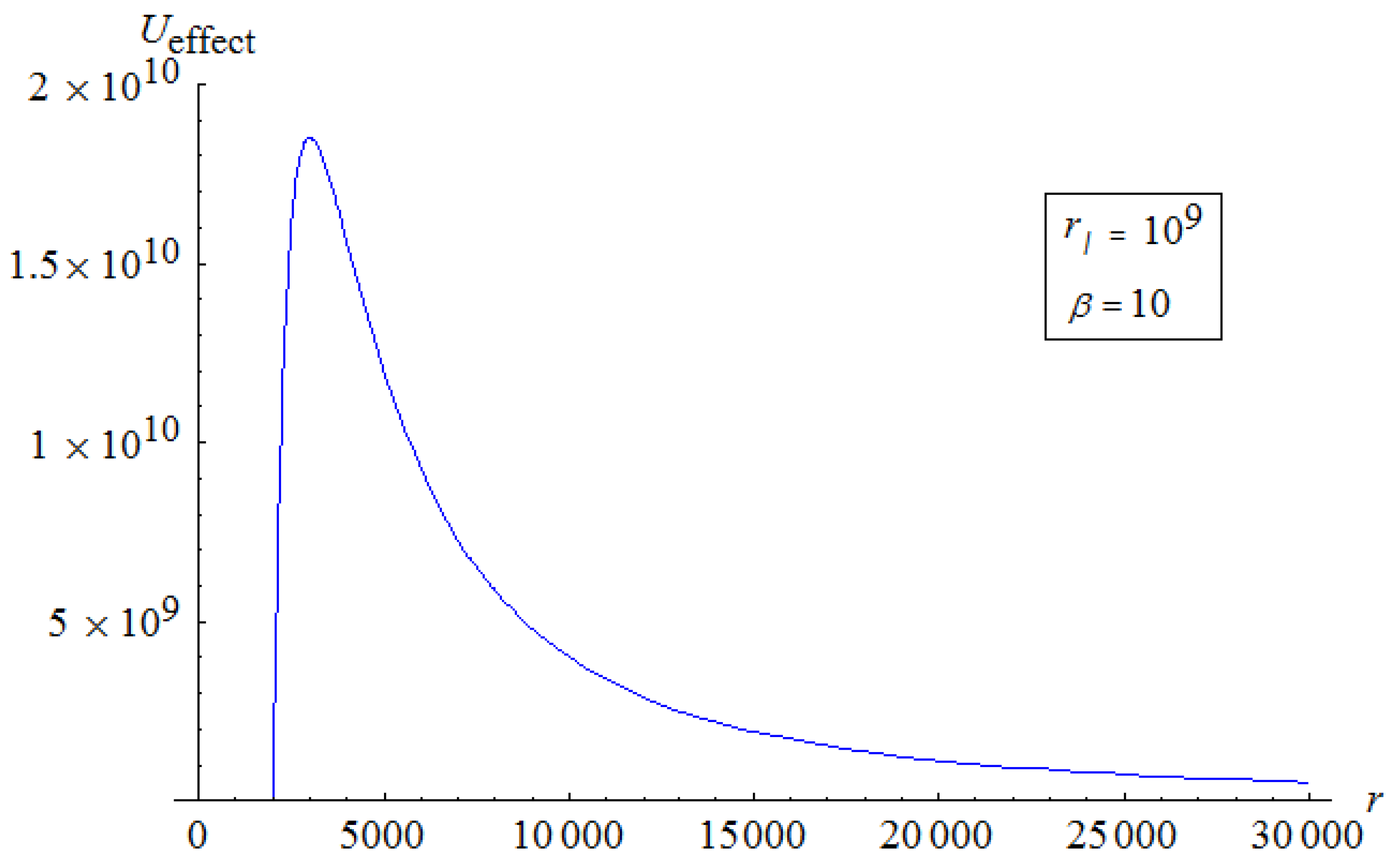
which corresponds to the second solution given in Equation (24). The Figure 1 illustrates the effective potential curve for scales where the gravitational radius is the dominant one. The second circular orbit located at (see Equation (24)) is not an exact solution of Equation (21) neither. This can be seen by replacing in Equation (21) and verifying that
evaluated at . In fact, becomes an exact solution only if the term (GR contribution) from Equation (21) is neglected. Then for large scales, under the assumption , as far as the cosmological constant effects are neglected, the effective potential () is defined by
ignoring then the GR contribution which mix the scales with L. In order to verify this assumption, we can calculate the extremal condition for the potential (32), obtaining then
from which we can obtain the result defined previously. The Figure 2 illustrates the effective potential curve at large scales under the condition . This portion of the curve corresponds to the stable orbit condition. This part of the effective potential will not suffer any modification when the cosmological constant effects are included.
The Case with 0
We can repeat the previous arguments. Then the full effective potential with the inclusion of the term is given by
At large scales, with , the previous potential can be approximated to
where again we have ignored the GR correction term due to the same arguments exposed previously. The condition in Equation (35) gives the condition
This is a reduced fourth order polynomial as has been defined in Appendix A. We can compare with the standard reduced form defined by Equation (A7). After following a standard procedure, we can define the discriminant for the quartic polynomial (36) as follows
in agreement with the result defined in Equation (A18) in Appendix B. This discriminant plays an analogous role to the root square term in a quadratic polynomial equation as it is the case in Equation (23). The type of solution obtained depends on the sign of the discriminant. In fact, it can be demonstrated that if , then there are no real solutions. If , we can get real solutions. Then represents a limit where we get the largest possible angular momentum such that still bound orbits are possible. The maximum angular momentum is defined by
This condition is coincident with the result obtained in [6]. The solutions for Equation (36), when , are defined by
The first solution is coincident with the second solution found for Equation (22). The second solution is new since it comes from the contribution, which was excluded previously. By using here the result (38), we can express as
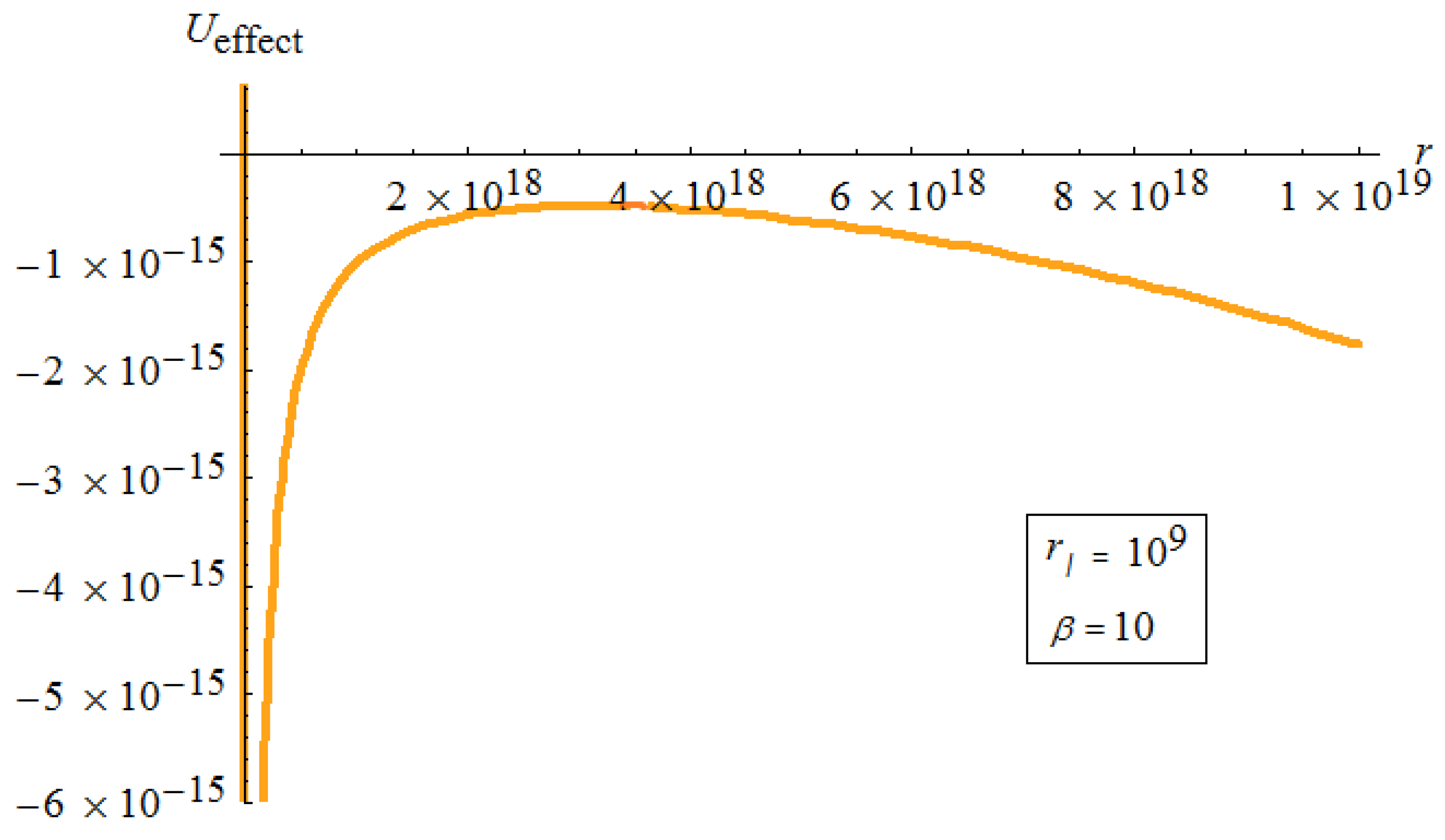
where . This solution corresponds to the local maximum illustrated in the Figure 3. The condition is equivalent to , which corresponds to a second saddle point condition different to the one defined previously for the result (25). This new saddle point is located at large scales defined by
4. The Role of in the Black-Hole Thermodynamics in S-dS Space
The black-hole surface gravity, can be defined as [3]
The labels BH and CH, correspond to the Black Hole Horizon and the Cosmological Horizon respectively. From Equation (18), the two horizons are the same when the mass of the Black Hole takes its maximum value given by
where corresponds to the Planck mass and . If the mass of a Black Hole is larger than the value given by Equation (44), then we have a naked singularity. As , the two event horizons are equally defined as . Then a thermodynamic equilibrium is established. As has been explained in [3], if , then the metric defined in Equation (1) obeys the condition everywhere. Then this coordinate system becomes inappropriate. In agreement with the results obtained in [26], we can select a better coordinate system by defining
where is a parameter related to the mass of the black-hole. In these coordinates, the degenerate case (when the two horizons become the same), corresponds to . We must then define the new radial and the new time coordinates to be
In these coordinates, the Black Hole horizon corresponds to and the Cosmological horizon to [3]. Then the metric (1) can be expressed as
after a standard coordinate transformation. The previous metric has been expanded up to first order in . Equation (47) is then the appropriate metric to be used as the mass of the Black Hole is near to its maximum value defined by Equation (44). For any value taken by the mass of the black-hole, the normalization of the time-like Killing vector corresponding to the conservation under time-translations is defined by
with being the normalization factor for the time-like Killing vector defined by
In an asymptotically flat space, it is standard to define when . However, for the S-dS case, since we can only define the static observer at the scale , then it is standard to normalize the time-like Killing vector as in Equation (49) with the factor defined by Equation (48). For the case with , where the angular momentum effects for the observer will appear, the corresponding corrections have to be done for the previous normalization factor. When the mass of the black hole satisfies , then in Equation (45) and the black-hole temperature takes its minimum possible value defined by
where is the surface gravity. Later we will see how in massive gravity theories, an analogous expression for the black-hole temperature appears. For any value taken by the black-hole mass, the black-hole temperature is defined by
where is the location of the static observer inside the S-dS solution. Other relevant analysis for the black-hole temperature in the S-dS solution in GR have been done in [3].
5. The Schwarzschild De-Sitter Solution in Massive Gravity
Here we will make a review of the derivation of the S-dS solution inside massive gravity. We then start by obtaining the field equations from the variation of the action
with the effective potential depending on two free parameters as
By convenience, here we redefine the free-parameters as follows
Here in addition
and
and then the field equations obtained from the variation of Equation (52) are defined as
The energy momentum tensor defined by
We can constraint the background solution to behave as the standard S-dS solution of GR. In such a case, the following result has to be satisfied
Then we get the solution
with
where . In this previous solution, all the degrees of freedom are inside the dynamical metric. The fiducial metric in this case is simply defined by Minkowski. It was found in [27,28] that the generic solution defined by Equation (64), can be classified in two families depending on the relation between the two free-parameters of the theory. The solutions are then defined as
5.1. Solution with a Degenerate Vacuum
In this particular solution, the condition is satisfied. Then the Stückelberg function defined by is arbitrary. For this case, the scale factor is defined as
and the cosmological constant, due to the constraint imposed in Equation (62) has to satisfy the condition
as can be easily verified.
5.2. Solution with Single Vacuum
For this solution, it was found that the function is constrained to behave as a solution of the following equation
Note that the solution for this equation has the Finkelstein form as has been demonstrated in [27,28]. In general the function has the following solution in this case
where is some function depending on spacetime. For the stationary case, only has dependence on r. In order to satisfy the constraint (67), here we have [27]
For this solution in addition, the scale factor is defined as
and the cosmological constant for this case is defined as
5.3. The Effective Potential in dRGT Massive Gravity
Having the generic solution for the spherically symmetric case, then we can proceed to calculate the equations of motion for a test particle moving under the influence of a spherically symmetric source inside the massive gravity formulation. Our derivation will be based in the solution formulated in Equation (64) for a general Stückelberg function . The equation to be analyzed is
Note that in this case the non-diagonal terms in the components will be relevant since we cannot gauge them away as in the GR case. Here instead of defining a conserved quantity in the direction of t, we define a conserved quantity in the direction of the Stückelberg function as follows
with . Here is a normalization factor, analogous to the one introduced in [3]. This previous relation is complemented with the standard conserved angular momentum already defined in Equation (12). Then in this case we obtain the following equation of motion for a test particle
Here A is a constant of motion. Then the potential will behave exactly as in the GR case, although there is a big difference in the behavior of the kinetic terms. In fact, for the case of massive gravity, the quantity associated to the time-translations is not conserved as in the case of GR. This can be observed from Equation (73). Here the conservation is only well defined in the direction of . Then what is in reality conserved is a combination of a quantity defined in the direction of the ordinary time t and a quantity defined in the spatial direction (r). Then although the potential term will have exactly the same behavior as in the case of GR, the combination of the kinetic term representing radial translations, together with the kinetic term representing temporal translations, will be combined such that their superposition (up to some factors), is a constant of motion. Then there is no conservation under time-translations in the usual sense in this case. This is a big difference with respect to the GR case, where there is conservation under ordinary time-translations. Another difference of the present case with respect to GR is how we define the scale for the potential (74). In this case, such scale will depend on the graviton mass and on the two free-parameters of the theory through the constants and [27]. It is not difficult to visualize that corresponds to the Vainshtein scale and it can be calculated in the same way as we did for the case of in GR. Then we can still use one of the solutions of the quartic equation defined in Equation (36) as the Vainshtein scale. The Vainshtein scale then becomes
up to some small corrections due to the angular momentum, analogous to the corrections found in Equation (40) for the case of ordinary gravity. Note that in this case and will take different values depending on the relations between the two free-parameters.
5.3.1. The Case of One Free-Parameter
In this case, and . Then
This scale clearly depends on the graviton mass [27].
5.3.2. The Case of Two Free-Parameters
In this case is a function of the two free-parameters as it has been defined in [27]. In addition
Then can be defined correspondingly.
6. Black-Hole Thermodynamics Inside the Non-Linear Formulation of Massive Gravity
The expression for the black-hole temperature inside the non-linear formulation of massive gravity for the S-dS solution, will not be different to the one defined previously for the GR case as far as we use the Killing vector in the direction of instead of using the ordinary time-like Killing vector as follows
Here we constraint . In addition, is the unit vector which marks the radial component of . is the normalization factor. We can now normalize this Killing vector as we did with the time-like Killing vector for the case of GR. Here however, the static observer is located at the scale corresponding to the Vainshtein scale and in order to agree with the GR results, this observer must define his/her time-coordinate in the direction of . This imposes some extra-constraints in the type of observers able to define the black-hole temperature as in GR. Any other observer defining a different notion of time, will disagree with the results obtained in GR, even if this observers is also located at the same scale. The difference will be more evident for observers located at larger scales than (in massive gravity) or (in GR). The notion of time then is an important concept in massive gravity and it is related to how we define the vacuum and the conservation laws. Here we normalize the Killing vector in the direction of as
Note that here since we are considering the Killing vector in the direction , then we have to consider the metric component in Equation (79). This component can be obtained from the result (64) if we rewrite the metric (63) as
where . If we compare the results (63) and (64) with Equation (80), then we conclude that . This justifies the previous results. Then we conclude that the normalization factor is
consistent with the result obtained inside GR in Equation (48). Note however that here we are normalizing the Killing vector in the direction instead of the Killing vector in the time-direction t. In addition the normalization is done with respect to the observers located at , namely, the Vainshtein scale. If we want to get the constraints for the Stückelberg function , consistent with the normalization (79) and with the conservation law (73), we have to expand Equation (79) in the alternative form
Here corresponds to the radial component of the metric living in the subspace formed by the vector . In other words, the components of the Killing vector in the direction of the Stückelberg function can be defined as
Here a and b define the components of inside a 2-dimensional subspace formed by and taken as unit vectors. This is the subspace where the conservation law (73) is valid. Then in general we can express , consistent with the definition (78). Then here in Equation (82). Taking into account this analysis, together with the solutions (64), then we find that Equation (82) can be simplified to
taking into account that inside the 2-dimensional subspace expanded by , and . If this previous result is consistent with Equation (79), then the following constraint has to be satisfied
This expression can be reduced as
This result is consistent with the conservation law defined in Equation (73) with the appropriate definitions for and . Within this scenario, the definition of surface gravity for black-holes in Massive gravity agrees with the standard definition of GR. This is true as far as the observers are constrained to move in the spacetime defined by the condition (85). This condition is general and it applies for both cases, namely, for the case where the vacuum is degenerate or for the case where the vacuum is single, taking into account that massive gravity is in essence a -model. The Stückelberg trick as has been used in this paper can be found in [29]. Note that the observers can define any location in space r or any notion of time t. In other words, they can move arbitrarily. However, those observers satisfying the constraint (85), will agree with the results of GR. For general motion, the results obtained from GR will disagree with the results obtained in massive gravity.
7. The Number of Propagating Degrees of Freedom and Lorentz Violation
The previous analysis has been based in solutions with non-trivial Stückelberg functions. In some scenarios this can be understood as Lorentz violating theories [30,31]. The Lorentz violation is, however, at the background level due to the non-triviality of the Stückelberg functions. This can be considered as spontaneous symmetry breaking, since the action itself still respects the violated symmetries. In the previous analysis, the number of degrees of freedom can fluctuates from two to five depending on how the observers define the notion of time. If an observer defines the time arbitrarily, then he/she will describe five degrees of freedom in general. On the other hand, the observers defining the time in agreement with the Stückelberg function , will describe two degrees of freedom. However, if we describe a black-hole with spherical symmetry, then we will not have tensor perturbations and we can just limit the analysis to three degrees of freedom in four dimensions. This can be perceived better if we expand the Lagrangian density in the action (52) up to second order. For simplicity we will work in a free falling frame where we can ignore the scales of gravity. This will help us to make a cleaner analysis. The free-falling condition here is different with respect to the one in GR because the dynamical metric in a free-falling frame does not necessarily goes to Minkowski, unless the Stückelberg function is trivial. By keeping the stationary condition, in a free-falling frame and for an arbitrary Stückelberg function, we get the dynamical
Here we will consider the non-trivial contribution as a radial fluctuation of the Stückelberg function. In this special case and is arbitrary. In general we can assume . If we consider small, then the radial fluctuations of the Stückelberg function inside the 2-dimensional subspace correspond to perturbations. Such fluctuations live inside the space where we defined the Killing vector . In general, the metric (87) is a consequence of the Stückelberg trick applied as
with and . If we expand , then is non-trivial and in the example developed here. By considering as perturbations, the dynamical metric would be Minkowski at the background level. The kinetic terms of the action will not change under the presence of the extra-degrees of freedom because they enter via the Stückelberg trick defined in Equation (88). This is the case because the Stückelberg trick looks like (but is completely different) a coordinate transformation from the GR perspective. Then we only have to worry about the perturbations of the massive action. In a free-falling frame, up to second order, the massive action is defined as
We can see that the radial fluctuations of the time-component of the Stückelberg function affects the number of degrees of freedom perceived by an observer. If becomes trivially the ordinary time coordinate, then the number of degrees of freedom is reduced to the ordinary case of GR taking into account that the massive term will become an ordinary cosmological constant. In conclusion, the number of degrees of freedom described by an observer will depend on the way how he/she defines the time coordinate with respect to the Stückelberg function. An observer defining , will perceive and will recover GR. Any other observer will perceive more degrees of freedom. Note that here for simplicity . A non-trivial contributions coming from will also affect the number of degrees of freedom perceived by observers. In addition, if we evaluate the second derivatives with respect to the graviton field in Equation (89), we will obtain a mass matrix. In such a case, the eigenvalues of the matrix would correspond to the masses of each mode, namely, , , etc. These are the mass fluctuations of the modes and they will depend on the non-trivial contributions of the Stückelberg function. In any other frame different to the free-falling one, the scales of gravity will appear but the analysis will be qualitatively the same. A similar analysis has been developed in [32,33] where massive gravity was analyzed as a gravitational -model.
8. Conclusions
In this paper, we have found the conditions which an observer in Massive gravity has to satisfy in order to agree with the black-hole temperature obtained originally in GR. The conditions impose some constraints in the functional behavior on the spacetime paths which the observers have to follow. The result is general in the sense that it is independent on whether the vacuum solution in massive gravity is single or degenerate, taking into account that massive gravity is a gravitational -model. The conditions to be satisfied by the Stückelberg fields come from the normalization of the Killing vector in the direction of defined previously in this paper. Note that the observers can take any arbitrary path in the spacetime. However, if they follow the paths marked by the constraints over the Stückelberg functions, as those defined in this paper, then they will find the same temperature as in GR inside the scenario of massive gravity. The analysis done in this paper illustrates in addition the coincidence between the scales in GR and in massive gravity. Other authors have derived some interesting analysis about the black-hole thermodynamics in massive gravity [34,35], however they did not consider the fact that in reality in massive gravity theories, the amount of particles emitted by the event horizon never changes. What in reality is different is the way how the observers define the notions of vacuum in massive gravity. For example, the modification for the black-hole temperatures found in [34,35] are correct as far as we consider arbitrary observers located at scales where the extra-degrees of freedom of the theory become relevant and in addition if the observers define the time direction arbitrarily. However, when the gravitational field is strong, the deviations with respect to GR must be small if the theory is consistent. For this reason, in [22,23], it was found that the periodicity of the poles of the propagator is distorted for the case of a scalar field moving around a source in massive gravity. This creates an apparent modification of the black-hole temperature in this theory. However, the reality is that if the observer defines the time coordinate in agreement with , such modifications with respect to GR disappear. In this paper in addition we have demonstrated that different observers can define different degrees of freedom depending on how they define the time-coordinate with respect to the Stückelberg function. An observer defining the local time in agreement with will define the same degrees of freedom as in GR. On the other hand, an observer defining the time arbitrarily with respect to will perceive more degrees of freedom. This is related to the way how we define the local masses for the different modes . These masses will depend on the non-trivial contributions coming from the Stückelberg function. By using these approaches, it would be interesting to analyze possible phase transitions for black-hole solutions in a similar way as has been done in [36]. Other interesting approaches have been developed in [37,38].
Acknowledgments
I.A. is supported by the JSPS Post Doctoral fellow for oversea researchers. I thank the referees of this paper for the important comments.
Conflicts of Interest
The author declares no conflict of interest.
Appendix A. General Solution of a Fourth-Order Polynomial
The standard form of a fourth-order equation can be taken to be
in order to get the reduced form of this equation, we need to do the following variable change
Solving for x, we get
Replacing this result inside of Equation (A1), we get
Developing parenthesis, we obtain
Regrouping common factors and dividing by A, we get
The standard reduced fourth-order equation is given by
Comparing this form with (A6), we obtain
The associated cubic equation of (A7) is
where P, Q and K are given in (A8). Given the solutions of the associated third-order Equation (A9), the solutions for the reduced Equation (A7) are given by
The solutions of the associated third-order Equation (A9), must satisfy the following
Appendix B. General Solution of a Third-Order Polynomy
The standard form of a third-order polynomy is given by
The normal form is obtained by dividing with respect to a the result as follows
where obviously, we have
with the extra condition . The reduced form of the third-order Equation (A13), requires the change of variable
and the reduced form is given by
with the corresponding coefficients given by
where r, s and t are given in (A14). On the other hand, it is necessary to establish a classification criteria for the reduced third-order equation given in (A16), the criteria is based in a parameter D given by
Also for the same classification, it is necessary to find an auxiliary parameter given by
where q and p are defined in eqns. (A16) and (A17). On the other hand, we define an auxiliary angle , which is defined depending of the following cases:
Case (i). .
In this case, the auxiliary angle is defined as
with the corresponding solutions
Case (ii). .
In this case, the auxiliary angle is defined as
and the corresponding solutions are
Case (iii). .
In this section, we define the auxiliary angle to be
with the corresponding solutions
In the mentioned three cases, D is defined in Equation (A18); p is defined in Equations (A16) and (A17), and the parameter R is defined in Equation (A19).
References
- Bażański, S.L.; Ferrari, V. Analytic Extension of the Schwarzschild-de Sitter Metric. Il Nuovo Cimento B 1986, 91, 126–142. [Google Scholar] [CrossRef]
- Arraut, I.; Batic, D.; Nowakowski, M. Comparing two approaches to Hawking radiation of Schwarzschild-de Sitter Black Holes. Class. Quantum Gravity 2009, 26, 125006. [Google Scholar] [CrossRef]
- Bousso, R.; Hawking, S.W. Pair creation of black holes during inflation. Phys. Rev. D 1996, 54, 6312–6322. [Google Scholar] [CrossRef]
- Bousso, R.; Hawking, S.W. (Anti)-evaporation of Schwarzschild-de Sitter black holes. Phys. Rev. D 1998, 57, 2436–2442. [Google Scholar] [CrossRef]
- Arraut, I. The Planck scale as a duality of the Cosmological Constant: S-dS and S-AdS thermodynamics from a single expression. arXiv, 2012; arXiv:1205.6905v3. [Google Scholar]
- Gibbons, G.W.; Hawking, S.W. Cosmological event horizons, thermodynamics and particle creation. Phys. Rev. D 1977, 15, 2738–2751. [Google Scholar] [CrossRef]
- Stuchlík, Z.; Slanký, P. Equatorial Circular orbits in the Kerr-de Sitter spacetimes. Phys. Rev. D 2004, 69, 064001. [Google Scholar] [CrossRef]
- Balaguera Antolinez, A.; Böhmer, C.G.; Nowakowski, M. Scales set by the Cosmological Constant. Class. Quantum Gravity 2006, 23, 485–496. [Google Scholar] [CrossRef]
- Babichev, E.; Deffayet, C. An introduction to the Vainshtein mechanism. Class. Quantum Gravity 2013, 30, 184001. [Google Scholar] [CrossRef]
- Vainshtein, A.I. To the problem of nonvanishing gravitation mass. Phys. Lett. B 1972, 39, 393–394. [Google Scholar] [CrossRef]
- Arraut, I.; Batic, D.; Nowakowski, M. Velocity and velocity bounds in static spherically symmetric metrics. Cent. Eur. J. Phys. 2011, 9, 926–938. [Google Scholar] [CrossRef]
- Stuchlík, Z. The motion of test particles in Black Hole Backgrounds with non-zero Cosmological Constant. Bull. Astron. Inst. Czech. 1983, 34, 129–149. [Google Scholar]
- Stuchlík, Z.; Hledík, S. Some properties of the Schwarzschild de-Sitter and Schwarzschild Anti de-Sitter spacetimes. Phys. Rev. D 1999, 60, 044006. [Google Scholar] [CrossRef]
- Stuchlík, Z. An Einstein Strauss de-Sitter model of the universe. Bull. Astron. Inst. Czech. 1984, 35, 205–215. [Google Scholar]
- Stuchlík, Z.; Calvani, M. Null geodesics in black hole metrics with non- zero Cosmological Constant. Gen. Relativ. Gravit. 1991, 23, 507–519. [Google Scholar] [CrossRef]
- Hua, C.J.; Jiu, W.Y. Inuence of Dark Energy on time-like geodesic motion in Schwarzschild spacetime. Chin. Phys. B 2008, 17, 1184–1188. [Google Scholar]
- Slanacutey, P.; Stuchlík, Z. Relativistic thick discs in Kerr- de Sitter backgrounds. Class. Quantum Gravity 2005, 22, 3623–3651. [Google Scholar]
- Kraniotis, G.V. Periapsis and gravitomagnetic precessions of stellar orbits in Kerr and Kerr-de Sitter black hole spacetimes. Class. Quantum Gravity 2007, 24, 1775–1808. [Google Scholar] [CrossRef]
- Kraniotis, G.V. Precise analytic treatment of Kerr and Kerr-(anti) de Sitter black holes as gravitational lenses. Class. Quantum Gravity 2011, 28, 085021. [Google Scholar] [CrossRef]
- Chauvineau, B.; Regimbau, T. Local effects of a Cosmological Constant. Phys. Rev. D 2012, 85, 067302. [Google Scholar] [CrossRef]
- Stuchlík, Z.; Slaný, P.; Hledík, S. Equilibrium configurations of perfect fluid orbiting Schwarzschild de-Sitter black holes. Astron. Astrophys. 2000, 363, 425–439. [Google Scholar]
- Arraut, I. On the apparent loss of predictability inside the de-Rham-Gabadadze-Tolley non-linear formulation of massive gravity: The Hawking radiation effect. Europhys. Lett. 2015, 109, 10002. [Google Scholar] [CrossRef]
- Arraut, I. Path-integral derivation of black-hole radiance inside the de-Rham-Gabadadze-Tolley formulation of massive gravity. arXiv, 2015; arXiv:1503.02150. [Google Scholar]
- Arraut, I. Komar mass function in the de Rham–Gabadadze–Tolley nonlinear theory of massive gravity. Phys. Rev. D 2014, 90, 124082. [Google Scholar] [CrossRef]
- Carroll, S. Space-Time and Geometry; Addison Wesley: Chicago, IL, USA, 2004. [Google Scholar]
- Ginsparg, P.; Perry, M.J. Semiclassical perdurance of de Sitter space. Nucl. Phys. B 1983, 222, 245–268. [Google Scholar] [CrossRef]
- Kodama, H.; Arraut, I. Stability of the Schwarzschild-de Sitter black hole in the dRGT massive gravity theory. Prog. Theor. Exp. Phys. 2014, 2014, 023E02. [Google Scholar] [CrossRef]
- Nowakowski, M.; Arraut, I. The minimum and maximum temperature of Black body radiation. Mod. Phys. Lett. A 2009, 24, 2133–2137. [Google Scholar] [CrossRef]
- Hinterbichler, K. Theoretical Aspects of Massive Gravity. Rev. Mod. Phys. 2012, 84, 671–710. [Google Scholar] [CrossRef]
- Rubakov, V.A.; Tinyakov, P.G. Infrared-modified gravities and massive gravitons. Phys. Usp. 2008, 51, 759–792. [Google Scholar] [CrossRef]
- Rubakov, V. Lorentz-violating graviton masses: getting around ghosts, low strong coupling scale and VDVZ discontinuity. arXiv, 2004; arXiv:hep-th/0407104. [Google Scholar]
- Arraut, I.; Chelabi, K. Non-linear massive gravity as a gravitational σ-model. Europhys. Lett. 2016, 115, 31001. [Google Scholar] [CrossRef]
- Arraut, I. The graviton Higgs mechanism. Europhys. Lett. 2015, 111, 61001. [Google Scholar] [CrossRef]
- Cai, R.-G.; Hu, Y.-P.; Pan, Q.-Y.; Zhang, Y.-L. Thermodynamics of black holes in massive gravity. Phys. Rev. D 2015, 91, 024032. [Google Scholar] [CrossRef]
- Vegh, D. Holography without translational symmetry. arXiv, 2013; arXiv:1301.0537v2. [Google Scholar]
- Fernando, S. Phase transitions of black holes in massive gravity. Mod. Phys. Lett. A 2016, 31, 1650096. [Google Scholar] [CrossRef]
- Hendi, S.H.; Li, G.Q.; Mo, J.X.; Panahiyan, S.; Panah, B.E. New perspective for black hole thermodynamics in Gauss–Bonnet–Born–Infeld massive gravity. Eur. Phys. J. C 2016, 76, 571. [Google Scholar] [CrossRef]
- Sanchez, A. Geometrothermodynamics of black holes in Lorentz noninvariant massive gravity. Phys. Rev. D 2016, 94, 024037. [Google Scholar] [CrossRef]
Figure 1.
The effective potential affecting the motion of a test particle at scales where the scale is important. Here is the ratio between the maximum angular momentum scale (to be defined later) and the ordinary angular momentum here defined as .
Figure 1.
The effective potential affecting the motion of a test particle at scales where the scale is important. Here is the ratio between the maximum angular momentum scale (to be defined later) and the ordinary angular momentum here defined as .

Figure 2.
Effective potential valid for scales satisfying and for a particular value of . The shape of the figure will not change for different values of . Here is the angular momentum scale.
Figure 2.
Effective potential valid for scales satisfying and for a particular value of . The shape of the figure will not change for different values of . Here is the angular momentum scale.
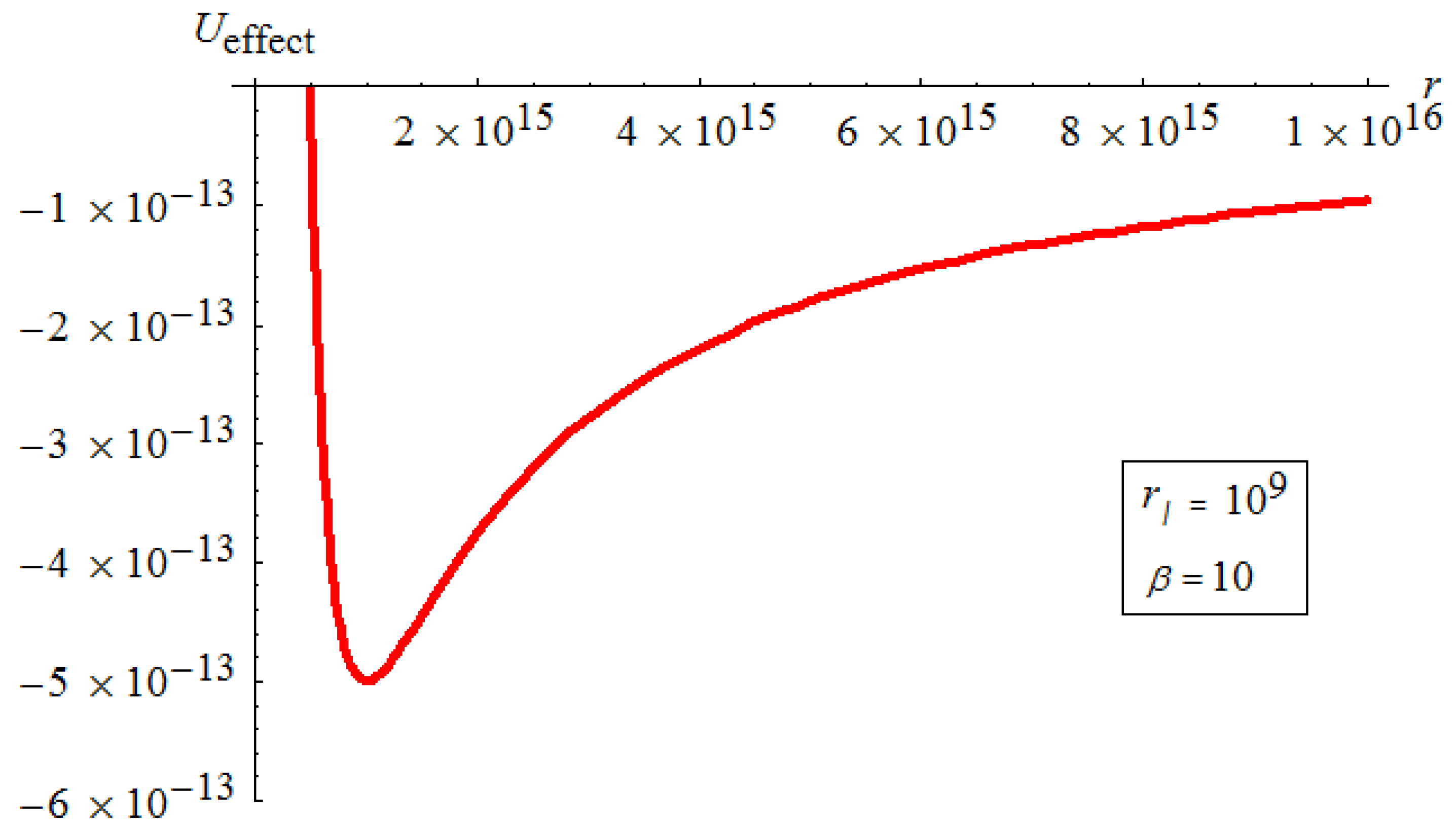
Figure 3.
Effective potential scales of the order and for some specific value of .

© 2017 by the author. Licensee MDPI, Basel, Switzerland. This article is an open access article distributed under the terms and conditions of the Creative Commons Attribution (CC BY) license (http://creativecommons.org/licenses/by/4.0/).
Share and Cite
MDPI and ACS Style
Arraut, I. The Astrophysical Scales Set by the Cosmological Constant, Black-Hole Thermodynamics and Non-Linear Massive Gravity. Universe 2017, 3, 45. https://doi.org/10.3390/universe3020045
AMA Style
Arraut I. The Astrophysical Scales Set by the Cosmological Constant, Black-Hole Thermodynamics and Non-Linear Massive Gravity. Universe. 2017; 3(2):45. https://doi.org/10.3390/universe3020045
Chicago/Turabian StyleArraut, Ivan. 2017. "The Astrophysical Scales Set by the Cosmological Constant, Black-Hole Thermodynamics and Non-Linear Massive Gravity" Universe 3, no. 2: 45. https://doi.org/10.3390/universe3020045
Note that from the first issue of 2016, this journal uses article numbers instead of page numbers. See further details here.