String-Inspired Gravity through Symmetries

Abstract

We study a string-inspired cosmological model from the symmetries point of view. We start by deducing the form that each physical quantity must take so that the field equations, in the string frame, admit self-similar solutions. In the same way, we formalize the use of power-law solutions (less restrictive than the self-similar ones) by studying the wave equation for the dilaton through the Lie group method. Furthermore, we show how to generate more solutions by using this approach. As examples, we calculate exact solutions to several cosmological models in the four-dimensional NS-NS (Neveu-Schwarz-Neveu-Schwarz) sector of low-energy effective string theory coupled to a dilaton and an axion-like H-field within the string frame background, with FRW and the Bianchi Type II metrics. We also study the existence of Noether symmetries, which allow us to determine the form of the physical quantities in the framework of FRW geometry and to find exact cosmological solutions.

1. Introduction

It is widely accepted that the classical or the modified gravitational theories break down near the initial singularity, when high energy phenomena are involved. In this way, it is necessary to develop new theories or models that are able to explain such phenomena. One such theory is the superstring theory, becoming a good candidate to unify all of the fundamental interactions, including the gravity [1,2]. We know five superstring models, the so-called: $I,IIA,IIB,$ $E_8\times E_8$ heterotic and $SO(32)$ heterotic, and there is now evidence that all of them are related, being different manifestations of a more fundamental theory known as M-theory [3].

The cosmological implications of superstring theory are currently attracting a great deal of attention. The starting point in any analysis is the low energy limit, since the theory predicts a classical gravitational interaction [4]. This gravitational theory differs from general relativity, in that it predicts the existence of a scalar field, known as the dilaton ϕ, and its potential V, the graviton, that is, the metric tensor and the antisymmetric tensor field strength ${\mathbf{H}}_{\mu \nu \lambda }$, which is a three-form, known as the Kalb–Ramond field.

The study of the cosmological consequences of superstring theory is quite important since the interactions of these fields permit us to obtain great deviations from the conventional gravitational models, i.e., the standard hot Big-Bang model (SHBB). This is why it is important to study whether the string models lead us to realistic cosmological scenarios that can explain the initial inflation, as well as other cosmological puzzles, as the large-scale structure formation or whether the cosmological solutions isotropize and/or homogenize towards the future.

Another important issue of the theory is motivated by the pre-Big-Bang scenarios [5], that is by the search of cosmological solutions that verify the symmetry $a(t)\to a^{-1}(-t)$ [6], being $a(t)$ the scale factor of the metric. Such a property is known as T-duality. As it has been pointed out in [6], if we do not take into account the potential $V,$ then the resulting field equations (FE) are invariant under the transformation $a(t)\to \widehat{a}(t)=a^{-1}(-t).$ However, if we assume a non-zero potential, $V\ne 0,$ in general, the FE are not invariant under the above symmetry, even if the solutions are invariant. In this paper, we do not consider this important part of the theory, focusing our attention in finding (and formalizing) exact solutions. Therefore, it would be necessary to have a fundamental method according to which the form (or forms) of the potential, as well as the other physical quantities could be fixed, and if it is possible, to calculate exact solutions to the proposed models. We have several geometric methods, such as: the matter collineation (self-similar solutions), Lie groups and Noether symmetries.

The study of self-similar (SS) models is quite important, since, as it has been pointed out by Rosquist and Jantzen [7], they correspond to equilibrium points, and therefore, a large class of orthogonal spatially-homogeneous models are asymptotically self-similar at the initial singularity and are approximated by exact perfect fluid or vacuum self-similar power-law models. Exact self-similar power-law models can also approximate general Bianchi models at intermediate stages of their evolution. This last point is of particular importance in relating Bianchi models to the real Universe. At the same time, self-similar solutions can describe the behavior of Bianchi models at late times i.e., as $t\to \infty ,$ playing a dominant role in the dynamics of Bianchi cosmological models (see Chapter X of [8] devoted to the study of string cosmological models through the dynamical system approach and the references therein). From the geometrical point of view, self-similarity is defined by the existence of a homothetic vector $\mathcal{H}$ in the spacetime, which satisfies the equation $L_{\mathcal{H}}{g}_{\mu \nu }=2\alpha g_{\mu \nu }$ [9]. The geometry and physics at different points on an integral curve of a homothetic vector field (HVF) differ only by a change in the overall length scale, and in particular, any dimensionless scalar will be constant along the integral curves. In this sense, the existence of an HVF is a weaker condition than the existence of a Killing vector field (KVF), since the geometry and physics are completely unchanged along the integral curves of a KVF.

The existence of self-similar solutions (which implies that the scale factor follows a power-law solution) is just a manifestation of scaling symmetries. It is opportune to point out that scaling is not the most general form of symmetry. Symmetry methods are arguably the most systematic way of dealing with exact solutions of differential equations (partial, as well as ordinary). In recent years, they have been successfully applied to various fields: gas dynamics, fluid mechanics, general relativity, etc. Amongst symmetries of a differential equation, those forming a one-parameter group of transformations can be determined algorithmically through the so-called Lie algorithm. Quite often, as in the string cosmological models, the field equations of the model contain arbitrary functions, whose functional forms cannot be fixed by any known laws. Since having symmetries is just a generic property, i.e., all equations do not admit symmetries, then symmetries can be used to classify such functions. This is known in the literature as group modeling [10]. The advantage of using such a technique is that it is systematic. Therefore, by studying the forms of the unknown functions for which the field equations admit symmetries, it is possible to uncover new integrable models. The importance of the power-law solutions in the framework of the string-inspired cosmological models has been pointed out for several authors, as for example Nojiri et al., in [11], and Elizalde et al., in [12].

Another method for determining the physical quantities is the use of Noether symmetries. The idea of using Noether symmetries as a cosmological tool is not new in this kind of study; for example, in [13], the authors proposed that the Noether point symmetry approach can be used as a selection rule for determining the form of the potential, that is they take into account the geometry of the field equations as a selection criterion, in order to fix the form of the potential. Dynamically speaking, Noether symmetries are considered to play a central role in physical problems, because they provide first integrals, which can be utilized in order to simplify a given system of differential equations and, thus, to determine the integrability of the system. There are several approaches to study these symmetries; the geometrical one (see, for instance, [14] and the references therein), the dynamical Noether symmetry approach based on the Lie group method [15,16] and the approach developed in [17,18]. In this paper, we shall follow the method proposed by Capozziello et al., in [14].

Therefore, the aim of this paper is to study the string-inspired cosmological model by using several symmetry methods in order to determine the form of the physical quantities, as for example the potential or the dilaton field. In particular, we are interested in studying whether self-similar solutions exist and how must each physical quantity behave in order that the FE admit such a class of solutions. We formulate and prove very general theorems, valid for all of the Bianchi models, as well as for the flat FRW one. In the same way, we formalize the use of power-law solutions (less restrictive than the self-similar ones) by studying the wave equation for the dilaton through the Lie group method. We also show how to use this approach in order to generate more solutions. Furthermore, we study the existence of Noether symmetries in order to determine the form of the potential, as well as to find exact solutions in the framework of the flat FRW geometry.

The paper is organized as follows. In Section 2, we introduce the low energy equations of motion in the string frame. We concentrate on four-dimensional cosmological models and describe the complete set of field equations taking into account a homogeneous $\mathbf{H}$-field. In Section 3, we state and proof a theorem, where we determine the exact form that each physical quantity may take in order that the FE admit exact self-similar solutions through the matter collineation approach. In Section 4, we formalize the use of power-law solutions (that is, the scale factor(s) behave(s) as $a_i(t)=t^a,$ $a\in \mathbb{R}$) by studying the wave equation for the dilaton through the Lie group method. We also show how to generate other solutions by using this approach. In Section 5, we study some examples by considering two metrics, the flat FRW and Bianchi Type II. For each metric, and working in the string frame, we find exact solutions to several cosmological scenarios where we take into account the interaction between the different fields, that is the dilaton with the potential, the $\mathbf{H}$-field and the graviton. In Section 6, we explore the Noether symmetry approach to determine the form of the physical quantities in the case of the FRW geometry. In the particular case being studied, we are able to calculate a complete general solution of the field equations. Section 7 is devoted to summarizing the conclusions. In the Appendix, we prove that the matter conservation is verified.

2. Field Equations

The action in four-dimensional spacetime from the low energy limit of string theory [19,20,21,22,23,24] is deduced by assuming a Ricci-flat compactification of the internal $(D-4)$-dimensional space decoupled from our four-dimensional spacetime [25,26,27] and adding the matter Lagrangian $L_{\mathrm{m}}$, which is decoupled from the dilaton field in the string frame; therefore, we start by considering the following action for strings in D-dimensions [4,6]:

$$S=\frac{1}{2{\kappa }^2}\int d^{4}x\sqrt{-g}{e}^{-\varphi }\left[R+{\left(\nabla \varphi \right)}^2-V-\frac{1}{12}{\mathbf{H}}^2\right]+\int d^{4}x\sqrt{-g}{\mathcal{L}}_{\mathrm{matter}}$$

(1)

being ${\kappa }^2=8\pi G$ a coupling constant. ϕ is the dilaton field determining the strength of the gravitational coupling, R is the scalar curvature and ${\mathbf{H}}_{\alpha \beta \delta }$, the Kalb–Ramond field, is the completely antisymmetric tensor field strength defined by $\mathbf{H}=dB$, where B is a rank-two antisymmetric tensor. ${\mathcal{L}}_{\mathrm{matter}}$ stands for the Lagrangian for the matter (a perfect fluid in this case). We also consider the potential V, and we assume that $V=V(\varphi ).$

The variation of this action with respect to the $g_{\mu \nu }$, $B_{\mu \nu }$ and ϕ, respectively, yields the field equations:

$$\begin{array}{cc}\hfill R_{\mu }^{\nu }-\frac{1}{2}{g}_{\mu }^{\nu }R& {=}^{\mathrm{eff}}{T}_{\mu }^{\nu }\hfill \end{array}$$

(2)

$$\begin{array}{cc}\hfill {\nabla }_{\mu }\left(e^{-\varphi }{\mathbf{H}}^{\mu \nu \lambda }\right)& =0\hfill \end{array}$$

(3)

$$\begin{array}{cc}\hfill 2\square \varphi +R-{\left(\nabla \varphi \right)}^2-V+{\partial }_{\varphi }V-\frac{1}{12}{\mathbf{H}}^2& =0\hfill \end{array}$$

(4)

$$\begin{array}{cc}\hfill {\nabla }_{\nu }\left({}^{(m)}{T}_{\mu }^{\nu }\right)& =0\hfill \end{array}$$

(5)

with ${\mathbf{H}}^2={\mathbf{H}}_{\mu \nu \lambda }{\mathbf{H}}^{\mu \nu \lambda }$ and where ${\mathbf{H}}_{\mu \nu \lambda }={\partial }_{[\mu }{B}_{\nu \lambda ]}$, $\square =g^{ab}{\nabla }_a{\nabla }_b$ is the d’Alembertoperator. We have defined:

$${}^{\mathrm{eff}}{T}_{\mu }^{\nu }{=}^{(m)}{T}_{\mu }^{\nu }{+}^{(\varphi )}{T}_{\mu }^{\nu }{+}^{(\mathbf{H})}{T}_{\mu }^{\nu }{+}^{(V)}{T}_{\mu }^{\nu }$$

(6)

with:

$$\begin{array}{cc}\hfill {}^{(m)}{T}_{\mu }^{\nu }& ={\kappa }^2{e}^{\varphi }{T}_{\mu }^{\nu }\hfill \end{array}$$

(7)

$$\begin{array}{cc}\hfill {}^{(\varphi )}{T}_{\mu }^{\nu }& =-\frac{1}{2}{g}_{\mu }^{\nu }{\left(\nabla \varphi \right)}^2+\left(g_{\mu }^{\nu }{g}^{\lambda \kappa }-g_{\mu }^{\lambda }{g}^{\nu \kappa }\right){\nabla }_{\lambda }{\nabla }_{\kappa }\varphi \hfill \end{array}$$

(8)

$$\begin{array}{cc}\hfill {}^{(\mathbf{H})}{T}_{\mu }^{\nu }& =\frac{1}{12}\left(3{\mathbf{H}}_{\mu \lambda \kappa }{\mathbf{H}}^{\nu \lambda \kappa }-\frac{1}{2}{g}_{\mu }^{\nu }{\mathbf{H}}^2\right)\hfill \end{array}$$

(9)

$$\begin{array}{cc}\hfill {}^{(V)}{T}_{\mu }^{\nu }& =-\frac{1}{2}{g}_{\mu }^{\nu }V\hfill \end{array}$$

(10)

note that $T_{\mu \nu }$ is the energy-momentum tensor derived from the matter Lagrangian (${\mathcal{L}}_{\mathrm{matter}}$).

Equation (4) may be replaced by the following one:

$$\square \varphi -{\left(\nabla \varphi \right)}^2-V-{\partial }_{\varphi }V+\frac{1}{6}{\mathbf{H}}^2+T=0$$

(11)

since:

$$R=-T-3\square \varphi +2{\left(\nabla \varphi \right)}^2+2V-\frac{1}{12}{\mathbf{H}}^2$$

(12)

In four dimensions, every three-form can be dualized to a pseudoscalar. Thus, an appropriated ansatz for the $\mathbf{H}$-field is:

$${\mathbf{H}}^{\mu \nu \lambda }=e^{\varphi }{ϵ}^{\mu \nu \lambda \kappa }{h}_{,\kappa }$$

(13)

where ${ϵ}^{\mu \nu \lambda \kappa }$ is the antisymmetric four-form (obeying ${\nabla }_{\rho }{ϵ}^{\mu \nu \lambda \kappa }=0$) and $h=h(t)$ is the Kalb–Ramond axion field. Then, the FE Equation (3) is satisfied automatically, and from the Bianchi identity $d\mathbf{H}=0$ for the antisymmetric field strengths, ${\mathbf{H}}_{\alpha \mu \nu }$ becomes the equation of motion for the scalar field h as (see [4,28,29,30,31]):

$$\square h+{\nabla }^{\mu }\varphi {\nabla }_{\mu }h=0$$

(14)

thus h evolves as a massless scalar field coupled to the dilaton.

In this paper, we consider that the matter content is described by a perfect fluid (PF), whose energy-momentum tensor is defined by:

$$T_{\mu \nu }=\left(\rho +p\right)u_{\mu }{u}_{\nu }+p{g}_{\mu \nu }$$

(15)

where ρ is the energy density of the fluid, p the pressure, and they are related by the equation of state $p=\gamma \rho ,$ $\left(\gamma \in (-1,1]\right)$, and $u^{\mu }=\left(1,0,0,0\right)$ is the four-velocity.

3. Self-Similarity Solutions: Matter Collineation Approach

Our purpose will be to determine the exact form that must follow each physical quantity in order for the field equations to admit self-similar (power-law) solutions. We shall use two tactics, the matter collineations approach, which guarantees us the existence of self-similar solutions, while with the Lie groups method (LGM), we study the existence of power-law solutions (less restrictive than the self-similar condition). Nevertheless, the LGM allows us to obtain more solutions, as we shall show in the next section. We begin by studying the field equations through the matter collineation approach following the method developed in a previous paper (see [32]).

In general relativity, the term self-similarity can be used in two ways. One is for the properties of space-times; the other is for the properties of matter fields. These are not equivalent in general. The self-similarity in general relativity was defined for the first time by Cahill and Taub [33] and Eardley [34] (see, for general reviews, [9,35]). Self-similarity is defined by the existence of a homothetic vector field V in the spacetime, which satisfies:

$$L_V{g}_{\mu \nu }=2\alpha g_{\mu \nu }$$

(16)

where $g_{\mu \nu }$ is the metric tensor, $L_V$ denotes Lie differentiation along the vector field $V\in \mathfrak{X}(M)$ and α is a constant. This is a special type of conformal Killing vector. This self-similarity is called homothety. If $\alpha \ne 0$, then it can be set to be unity by a constant rescaling of V. If $\alpha =0$, i.e., $L_V{g}_{ij}=0$, then V is a Killing vector.

Homothety is a purely geometric property of spacetime, so that the physical quantity does not necessarily exhibit self-similarity, such as $L_{V}Z=kZ$, where k is a constant and Z is, for example, the pressure, or the energy density, and so on. From Equation (16), it follows that $L_V{R}^{\alpha }{}_{\mu \nu \lambda }=0,$ and hence, $L_V{R}_{\mu \nu }=0$ and $L_V{G}_{\mu \nu }=0.$ A vector field V that satisfies the above equations is called a curvature collineation, a Ricci collineation and a matter collineation, respectively. It is noted that such equations do not necessarily mean that V is a homothetic vector. For example, if we consider the Einstein equations $G_{\mu \nu }=8\pi G{T}_{\mu \nu },$ where $T_{\mu \nu }$ is an effective stress-energy tensor, then if the spacetime is homothetic, the energy-momentum tensor of the matter fields must satisfy $L_V{T}_{ij}=0$; nevertheless, in this work, we are not interested in finding the set of vector fields $V\in \mathfrak{X}(M)$ that verify such an equation, otherwise, knowing that the homothetic vector field (HVF) $\mathcal{H}$ (see for example [9]), that is $L_{\mathcal{H}}{g}_{\mu \nu }=2g_{\mu \nu },$ then $\mathcal{H}$ is also a matter collineation, i.e., $L_{\mathcal{H}}{T}_{\mu \nu }=0,$ then we use this fact to determine the behavior of the main physical quantities in order that the field equations admit self-similar solutions (see [35]).

Therefore, we calculate:

$$L_{\mathcal{H}}{T}_{\mu \nu }^{\mathrm{eff}}=0$$

(17)

where $\mathcal{H}$ is a homothetic vector field (HVF), i.e., it verifies the equation: $L_{\mathcal{H}}{g}_{\mu \nu }=2g_{\mu \nu },$ for some metric and where $T_{\mu \nu }^{\mathrm{eff}}$ is the effective stress-energy tensor. For this purpose, we have shown in [32] that it is enough to calculate $L_{\mathcal{H}}{}^{(i)}{T}_{\mu \nu }=0,$ for each component of the stress-energy tensor. For simplicity, and without lost of generality, we consider an FRW metric; thus, the HVF yields (see, for instance, [36]):

$$\mathcal{H}=t{\partial }_t+\left(1-a_1\right)\left(x{\partial }_x+y{\partial }_y+z{\partial }_z\right)$$

(18)

where $a_1\in \mathbb{R}$ is a numerical constant, while for example, the HVF for the BII metric yields:

$$\mathcal{H}=t{\partial }_t+\left(1-a_1\right)x{\partial }_x+\left(1-a_2\right)y{\partial }_y+\left(1-a_3\right)z{\partial }_z$$

(19)

with $a_1,a_2,a_3\in \mathbb{R}.$ We may do such simplification because, as we have shown in [32], all of the physical quantities are homogeneous, that is they only depend on time $t,$ then, the unique equation of $L_{\mathcal{H}}^{(i)}{T}_{\mu \nu }=0$, that is interesting for us, is the one corresponding to the temporal coordinate $t{\partial }_t.$ For this reason, the theorems that we are going to state are absolutely general for all of the Bianchi types and the FRW one.

We determine the exact form that each physical quantity must take in order that the FE admit SS solutions in the string frame. To do that, we study the effective stress-energy tensor through the matter collineation approach.

Theorem 1. 

The FE (Equations (2)–(5)) admits SS solutions if the physical quantities take the following form:

$$\rho ={\rho }_0{t}^{-\left(2+{\varphi }_0\right)},\varphi ={\varphi }_{0}lnt,h=h_0{t}^{-{\varphi }_0}+h_1,V=\mathsf{\Lambda }{e}^{-\frac{2}{{\varphi }_0}\varphi }$$

where ${\rho }_0,{\varphi }_0,h_0,h_1,\mathsf{\Lambda }$ are constants.

Proof. 

We split the effective stress-energy tensor into the following components:

$$\begin{array}{cc}\hfill {}^{(m)}{T}_{\mu }^{\nu }& =e^{\varphi }{T}_{\mu }^{\nu }\hfill \end{array}$$

(20)

$$\begin{array}{cc}\hfill {}^{(\varphi )}{T}_{\mu }^{\nu }& =\frac{1}{2}{g}_{\mu }^{\nu }\left[2{\nabla }^2\varphi -{\left(\nabla \varphi \right)}^2\right]-{\nabla }_{\mu }{\nabla }^{\nu }\varphi \hfill \end{array}$$

(21)

$$\begin{array}{cc}\hfill {}^{(\mathbf{H})}{T}_{\mu }^{\nu }& =\frac{1}{12}\left(3{\mathbf{H}}_{\mu \lambda \kappa }{\mathbf{H}}^{\nu \lambda \kappa }-\frac{1}{2}{g}_{\mu }^{\nu }{\mathbf{H}}^2\right)\hfill \end{array}$$

(22)

$$\begin{array}{cc}\hfill {}^{(V)}{T}_{\mu }^{\nu }& =-\frac{1}{2}{g}_{\mu }^{\nu }V\hfill \end{array}$$

(23)

In the string frame, we calculate the following equations ($L_{\mathcal{H}}^{(i)}{T}_{\mu \nu }=0$);

$$\begin{array}{cc}\hfill t\rho {\varphi }^{\prime }+t{\rho }^{\prime }+2\rho & =0,L_{\mathcal{H}}^{(m)}{T}_{\mu \nu }=0\hfill \end{array}$$

(24)

$$\begin{array}{cc}\hfill t\left({\varphi }^{″}\left(3H-{\varphi }^{\prime }\right)+3{\varphi }^{\prime }\left(\frac{a^{″}}{a}-H^2\right)\right)+6{\varphi }^{\prime }H-{\varphi }^{\prime 2}& =0,L_{\mathcal{H}}^{(\varphi )}{T}_{\mu \nu }=0\hfill \end{array}$$

(25)

$$\begin{array}{cc}\hfill t{h}^{\prime }{\varphi }^{\prime }+t{h}^{″}+h^{\prime }& =0,L_{\mathcal{H}}^{(\mathbf{H})}{T}_{\mu \nu }=0\hfill \end{array}$$

(26)

$$\begin{array}{cc}\hfill V_{\varphi }t{\varphi }^{\prime }+2V& =0,L_{\mathcal{H}}^{(V)}{T}_{\mu \nu }=0\hfill \end{array}$$

(27)

Note that our matter collineation vector field is the homothetic one, this means that the scale factor behaves as $a=a_0{t}^{a_1},$ $a_0=1$ and $a_1\in {\mathbb{R}}^{+}.$ Thus, from Equation (25), we get:

$$\varphi =\int \frac{3t{a}^{\prime }\pm \sqrt{9t^2{a}^{\prime 2}-2a^2{C}_1}}{ta}dt$$

(28)

and taking into account that the scale factor must behave as $a=a_0{t}^{a_1},$ then we get:

$$\varphi =C_1+C_{2}lnt,C_1,C_2\in \mathbb{R}$$

(29)

but within the framework of SS solutions, we choose the particular solution $\varphi ={\varphi }_{0}lnt,$ by setting $C_1=0,$ without lost of generality. From Equation (27), we get:

$$V_{\varphi }t{\varphi }^{\prime }+2V=0⟹V=\mathsf{\Lambda }{e}^{-\frac{2}{{\varphi }_0}\varphi }$$

(30)

where $\mathsf{\Lambda }=V_0$ is an integration constant, while from Equation (26):

$$t{h}^{″}+\left({\varphi }_0+1\right)h^{\prime }=0⟹h=h_0{t}^{-{\varphi }_0}+h_1,h_1,h_0\in \mathbb{R}$$

(31)

where we may set $h_1=0,$ within the SS framework. To end, we calculate the behavior of the energy density, finding that:

$$t{\rho }^{\prime }+\left(2+{\varphi }_0\right)\rho =0⟹\rho ={\rho }_0{t}^{-\left(2+{\varphi }_0\right)}$$

(32)

Therefore it is possible to find SS solutions if the main quantities behave as follows:

$$\rho ={\rho }_0{t}^{-\left(2+{\varphi }_0\right)},\varphi ={\varphi }_{0}lnt,h=h_0{t}^{-{\varphi }_0}+h_1,V=\mathsf{\Lambda }{e}^{-\frac{2}{{\varphi }_0}\varphi }$$

(33)

as it is required. The constants ${\rho }_0,{\varphi }_0,h_0,h_1$ and Λ are determined by solving the FE. ☐

4. Lie Groups

We have proven how each physical quantity must behave under the hypothesis of self-similarity. In the next section, we shall see that sometimes this condition results in being very restrictive, and for this reason, we may only be interested in finding power-law solutions. In order to try to generalize the self-similar results, we go next to work under the hypothesis of the power-law solution for the scale factor(s) (less restrictive than the self-similar hypothesis). To do that, we study through the Lie group method the wave equation for the dilaton.

Roughly speaking, a symmetry, $X=\xi (x,y){\partial }_x+\eta (x,y){\partial }_y,$ of a differential equation is an invertible transformation that leaves it form-invariant. By applying the standard Lie procedure (see, for instance, [16,37,38]), we need to solve the following overdetermined system of linear partial differential equations for η and ξ (from the extended infinitesimal or prolonged transformations), which allows us to determine the set of the symmetries admitted by Equation (4).

Equation (4) is of the general form.

$${\varphi }^{″}=f(t,\varphi ,{\varphi }^{\prime })$$

(34)

$f(t,\varphi ,{\varphi }^{\prime })=-2K{\varphi }^{\prime }\theta +R+{\varphi }^{\prime 2}-\frac{1}{2}{e}^{2\varphi }{h}^{\prime 2}-V+V_{\varphi },$ with $\theta =u_{;i}^i,$ $u^i=(1,0,0,0)$ (see below for details). We are going now to apply all of the standard procedures of Lie group analysis to this equation (see [37] for details and notation). A vector field X:

$$X=\xi (t,\varphi ){\partial }_t+\eta (t,\varphi ){\partial }_{\varphi }$$

(35)

is a symmetry of Equation (34) if:

$$\begin{array}{c}-\xi f_t-\eta f_{\varphi }+{\eta }_{tt}+\left(2{\eta }_{t\varphi }-{\xi }_{tt}\right){\varphi }^{\prime }+\left({\eta }_{\varphi \varphi }-2{\xi }_{t\varphi }\right){\varphi }^{\prime 2}-{\xi }_{\varphi \varphi }{\varphi }^{\prime 3}+\\ +\left({\eta }_{\varphi }-2{\xi }_t-3{\varphi }^{\prime }{\xi }_{\varphi }\right)f-\left[{\eta }_t+\left({\eta }_{\varphi }-{\xi }_t\right){\varphi }^{\prime }-{\varphi }^{\prime 2}{\xi }_{\varphi }\right]f_{{\varphi }^{\prime }}=0\end{array}$$

(36)

Thus, our approach consists of imposing a particular symmetry and deducing the exact form that acquires the unknown functions, that is ϕ, V and h, by solving the system of PDEs (Equation (36)). The imposed symmetry induces a change of variables, which usually reduces Equation (34) to an integrable ODE. However, sometimes, it is not possible to find a solution of such an ODE; for this reason, the knowledge of one symmetry X might suggest the form of a particular solution as an invariant of the operator X, i.e., a solution of $dt/\xi (t,\varphi )=d\varphi /\eta (t,\varphi ).$ This particular solution is known as an invariant solution (generalization of similarity solution).

Therefore, we study the equation:

$$2\square \varphi +R-{\left(\nabla \varphi \right)}^2-V+{\partial }_{\varphi }V-\frac{1}{12}{\mathbf{H}}^2=0$$

(37)

that we rewrite as follows:

$$2{\varphi }^{″}+2K{\varphi }^{\prime }\theta -R-{\varphi }^{\prime 2}+\frac{1}{2}{e}^{2\varphi }{h}^{\prime 2}+V-V_{\varphi }=0$$

(38)

where $\theta =u_{;i}^i,$ $u^i=(1,0,0,0).$ We use the notation ${\varphi }^{\prime }=\frac{d}{dt}\varphi ,$ $V_{\varphi }=\frac{d}{d\varphi }V,$ etc. Compare Equation (38) to Equation (60) for the FRW model and to Equation (82) for the Bianchi Type II model.

Theorem 2. 

The FE (Equations (2)–(5)) admit power-law solutions if the physical quantities take the following form:

$$\varphi ={\varphi }_{0}lnt,h=h_0{t}^{-{\varphi }_0}+h_1,V=\mathsf{\Lambda }{e}^{-\frac{2}{{\varphi }_0}\varphi }$$

Proof. 

By studying through the LG method Equation (38), we get:

$$\begin{array}{c}2{\xi }_{\varphi \varphi }+{\xi }_{\varphi }=0\end{array}$$

(39)

$$\begin{array}{c}8K\theta {\xi }_{\varphi }-2{\eta }_{\varphi }+4{\eta }_{\varphi \varphi }-8{\xi }_{t\varphi }=0\end{array}$$

(40)

$$\begin{array}{c}3\left(2V-2R-2V_{\varphi }+e^{2\varphi }{h}^{\prime 2}\right){\xi }_{\varphi }+4K\left(\theta {\xi }_t+\xi {\theta }^{\prime }\right)-4{\eta }_t+8{\eta }_{t\varphi }-4{\xi }_{tt}=0\end{array}$$

(41)

$$\begin{array}{c}2e^{2\varphi }\left(h^{\prime }{h}^{″}\xi +h^{\prime 2}\left({\xi }_t-{\eta }_{\varphi }+\eta \right)\right)+4K\theta {\eta }_t+4{\eta }_{tt}-2\eta V_{\varphi \varphi }\\ +2V_{\varphi }\left(\eta -2{\xi }_t+{\eta }_{\varphi }\right)+2V\left(2{\xi }_t+{\eta }_{\varphi }\right)-2R^{\prime }\xi -2R\left(2{\xi }_t-{\eta }_{\varphi }\right)=0\end{array}$$

(42)

Now, we impose the symmetry $\left[\xi =at,\eta =1\right],$ $a\in \mathbb{R},$ which brings us to get the following restrictions on the potential, $V,$ and the other quantities $\theta ,$ R and $h.$ From Equation (41), we obtain:

$$\theta {\xi }_t+\xi {\theta }^{\prime }=0\theta =\frac{c}{t},c\in \mathbb{R}$$

and splitting Equation (42):

$$\begin{array}{cc}\hfill 2e^{2\varphi }\left(h^{\prime }{h}^{″}\xi +h^{\prime 2}\left({\xi }_t-{\eta }_{\varphi }+\eta \right)\right)& =0\hfill \end{array}$$

(43)

$$\begin{array}{cc}\hfill -2\eta V_{\varphi \varphi }+2V_{\varphi }\left(\eta -2{\xi }_t+{\eta }_{\varphi }\right)+2V\left(2{\xi }_t+{\eta }_{\varphi }\right)& =0\hfill \end{array}$$

(44)

$$\begin{array}{cc}\hfill -2R^{\prime }\xi -2R\left(2{\xi }_t-{\eta }_{\varphi }\right)& =0\hfill \end{array}$$

(45)

so:

$$\begin{array}{cc}\hfill h^{″}at+h^{\prime }\left(a+1\right)& =0\hfill \end{array}$$

(46)

$$\begin{array}{cc}\hfill V_{\varphi \varphi }+V_{\varphi }\left(2a-1\right)-2aV& =0\hfill \end{array}$$

(47)

$$\begin{array}{cc}\hfill R^{\prime }t+2R& =0\hfill \end{array}$$

(48)

Therefore, we have obtained the following solutions:

$$\theta =\frac{c}{t},R=r{t}^{-2},V=C_1{e}^{-2a\varphi }+C_2{e}^{\varphi },h=C_3{t}^{-\frac{1}{a}}-C_4$$

(49)

where $c,r,{\varphi }_0,C_i\in \mathbb{R}.$ By taking into account physical and dimensional considerations, we reach the following results:

$$\theta =\frac{c}{t},R=r{t}^{-2},V=V_0{e}^{-\frac{2}{{\varphi }_0}\varphi },h=h_0{t}^{-{\varphi }_0}+h_1$$

(50)

For example, by setting $C_2=0,$ we conclude that a particular solution for the potential function is given by:

$$V=V_0{e}^{-\frac{2}{{\varphi }_0}\varphi }$$

(51)

where $V_0$ is an integration constant; in this way, we obtain a decreasing potential, and to obtain $V\approx t^{-2},$ since $G_{\mu \nu }\approx t^{-2}$ and therefore, each component of the FE must behave as $\approx t^{-2}.$ Now, by introducing these results into Equation (38), it reads:

$$2{\varphi }_{tt}+2K{\varphi }_t{t}^{-1}-{\varphi }_t^2+\frac{h_0^2{\varphi }_0^2}{2}{e}^{2\varphi }{t}^{-2\left({\varphi }_0+1\right)}+\left(1+\frac{2}{{\varphi }_0}\right)V_0{e}^{-\frac{2}{{\varphi }_0}\varphi }-r{t}^{-2}=0$$

(52)

where the symmetry $\left[at,1\right]$ induces the following change of variables,

$$x=\varphi -{\varphi }_{0}lnt,y=\frac{1}{t{\varphi }^{\prime }-{\varphi }_0}$$

(53)

getting in this way an Abel equation:

$$y^{\prime }=\left(l{e}^{-\frac{2}{{\varphi }_0}x}+\frac{h_0}{4}{e}^{2x}+A_1\right)y^3+A_2{y}^2-\frac{1}{2}y$$

(54)

with $l=1/2+1/{\varphi }_0,A_1=K{\varphi }_0-r/2-{\varphi }_0^2/2-{\varphi }_0$ and $A_2=K-1-{\varphi }_0,$ which has no solution. Therefore, the invariant solution, induced by the symmetry, of Equation (52) is:

$$\varphi ={\varphi }_{0}lnt$$

(55)

which is a particular solution of Equation (52). Therefore, the invariant solution coincides with the homothetic one. ☐

In order to show how useful this tactic is, we may consider another symmetry, for example $\left[a,1\right],$ $a\in \mathbb{R}$. Therefore, following the same steps as in the above proof, we get from Equation (41):

$${\theta }^{\prime }=0\theta =const$$

and splitting Equation (42), we get:

$$\begin{array}{cc}\hfill 2e^{2\varphi }\left(h^{\prime }{h}^{″}\xi +h^{\prime 2}\left({\xi }_t-{\eta }_{\varphi }+\eta \right)\right)& =0,h^{″}a+h^{\prime }=0\hfill \\ \hfill -2\eta V_{\varphi \varphi }+2V_{\varphi }\left(\eta -2{\xi }_t+{\eta }_{\varphi }\right)+2V\left(2{\xi }_t+{\eta }_{\varphi }\right)& =0,V_{\varphi \varphi }-V_{\varphi }=0\hfill \\ \hfill -2R^{\prime }\xi -2R\left(2{\xi }_t-{\eta }_{\varphi }\right)& =0,R^{\prime }=0\hfill \end{array}$$

in this way, we get the following invariant solution:

$$\varphi =\frac{1}{a}t,\theta =const,R=const,V=C_1+C_2{e}^{\varphi },h=C_3{e}^{-\frac{1}{a}t}-C_4$$

where $a,r,{\varphi }_0,C_i\in \mathbb{R}$, and from physical considerations, we set:

$$\varphi ={\varphi }_{0}t,\theta =const,R=r,V=V_0,h=h_0{e}^{-{\varphi }_{0}t}=h_0{e}^{-\varphi }$$

where the solution $\theta =const$, lead us to obtain:

$$\theta =c=\frac{a^{\prime }}{a},a=e^{a_{1}t},q=\frac{d}{dt}(H^{-1})-1=-1$$

note that this solution verifies the $T-$duality symmetry property $\left(a(t)\to a^{-1}(-t)\right)$. Now, we try to find a general solution for the dilaton from the WEEquation (38); thus:

$$2{\varphi }^{″}+2Kc{\varphi }^{\prime }-r-{\varphi }^{\prime 2}+\frac{1}{2}{e}^{2\varphi }{h}_0{e}^{-t/a}+V_0=0$$

where $\varphi ={\varphi }_{0}t$ is a particular solution. For simplicity, in the FRW case, see below for details, we find that:

$${\rho }^{\prime }+\left(1+\gamma \right)\rho a_1=0,\rho ={\rho }_0{e}^{-\left(1+\gamma \right)a_{1}t}$$

and therefore, we obtain as the solution:

$$\varphi =t,\theta =const,a=e^{a_{1}t},R=const,V=V_0,h=h_0{e}^{-t},\rho ={\rho }_0{e}^{-t}$$

where $\left(1+\gamma \right)a_1=1,$ that is: $a_1=\frac{1}{1+\gamma },$ with $\gamma \in (-1,1].$ Therefore, this solution is inflationary, $q=-1$, verifies the $T-$duality property and has a constant potential, $V=V_0.$

5. Examples

Once we have determined which is the behavior of each physical quantity, we go next to study some particular examples working in the string frame. We have chosen this frame for working since in the presence of matter, the frame change of metric makes the dilaton field ϕ couple with matter fields differently depending on their spins and the matter energy-momentum tensors to be non-trivial functions of the dilaton field. Thus, we use the fundamental string frame as it is in the action Equation (1) [39].

As the first example, we consider flat homogeneous an isotropic FRW metric, while for the second one, we take into account the homogeneous, but anisotropic Bianchi Type II metric. We consider some different cosmological scenarios by taking into account the different fields, the dilaton, the potential, a homogeneous $\mathbf{H}$-field (${\mathbf{H}}_{\mu \nu \lambda }$) and the matter field. We start by considering only the dilaton and go next to study more complex situations. We shall work only in the string frame, outlining the FE and calculating the exact self-similar solutions to each model.

5.1. Models with the Flat FRW Metric

For the usual flat FRW metric:

$$d{s}^2=-d{t}^2+a^2(t)\sum _{i=1}^3{\left(d{x}^i\right)}^2$$

(56)

with $a(t)=t^{a_1},$ $a_1\in \mathbb{R}$ (since we are working under the SS hypothesis), we find the following FE in the string frame:

$$\begin{array}{cc}\hfill 3H^2& =e^{\varphi }\rho -\frac{1}{2}{\varphi }_t^2+3H{\varphi }_t+\frac{1}{4}{e}^{2\varphi }{h}_t^2+\frac{1}{2}V(\varphi )\hfill \end{array}$$

(57)

$$\begin{array}{cc}\hfill 2H^{\prime }+3H^2& =-e^{\varphi }p+{\varphi }_{tt}+2H{\varphi }_t-\frac{1}{2}{\varphi }_t^2-\frac{1}{4}{e}^{2\varphi }{h}_t^2+\frac{1}{2}V(\varphi )\hfill \end{array}$$

(58)

$$\begin{array}{cc}\hfill h_{tt}+h_t\left(3H+{\varphi }_t\right)& =0\hfill \end{array}$$

(59)

$$\begin{array}{cc}\hfill 2{\varphi }_{tt}+6H{\varphi }_t-{\varphi }_t^2-R+V-{\partial }_{\varphi }V+\frac{1}{2}{e}^{2\varphi }{h}_t^2& =0\hfill \end{array}$$

(60)

with:

$$H=\frac{a^{\prime }}{a},\text{and}R=6\left(H^2+\frac{a^{″}}{a}\right)$$

(61)

and the conservation equation for the matter field:

$${\rho }^{\prime }+\left(1+\gamma \right)\rho \theta =0$$

(62)

where $\theta =u_{;i}^i$, $u^i=(1,0,0,0).$ Recall that the main physical quantity behaves as follows:

$$a=t^{a_1},\rho ={\rho }_0{t}^{-\left({\varphi }_0+2\right)},\varphi ={\varphi }_{0}lnt,h=h_0{t}^{-{\varphi }_0}+h_1,V=\Lambda e^{-\frac{2}{{\varphi }_0}\varphi }$$

(63)

note that from Equation (62) and $\rho ={\rho }_0{t}^{-\left({\varphi }_0+2\right)}$, we obtain the following relationship between the coefficients: $a_1\left(1+\gamma \right)=\left({\varphi }_0+2\right).$ We would like to emphasize that it is also possible to enlarge this study to the non-flat FRW models, but with the drawback that in these cases, the self-similar solution is only valid for the value of the equation of state (EoS) $\gamma =-1/3.$

We have found the following exact solutions for the next string cosmological models:

(1)

We begin by taking into account only the dilaton field; thus, the effective stress-energy tensor is defined by: ${}^{\mathrm{eff}}{T}_{\mu \nu }={}^{(\varphi )}{T}_{\mu \nu },$ neglecting the influence of other fields. In this case, the field equations are greatly simplified:

$$\begin{array}{cc}\hfill 3H^2& =-\frac{1}{2}{\varphi }_t^2+3H{\varphi }_t\hfill \end{array}$$

(64)

$$\begin{array}{cc}\hfill 2H^{\prime }+3H^2& ={\varphi }_{tt}+2H{\varphi }_t-\frac{1}{2}{\varphi }_t^2\hfill \end{array}$$

(65)

$$2{\varphi }_{tt}+6H{\varphi }_t-{\varphi }_t^2-R=0$$

(66)

We found the following solution:

$$a(t)=t^{\sqrt{3}/3},\varphi =\left(\sqrt{3}-1\right)ln\left|t\right|$$

(67)

This solution has been found by many authors (see, for instance, [40,41]). In this paper, we are only interested in studying the solutions for $t\in {\mathbb{R}}^{+}.$ We see that the deceleration parameter is: $q=\sqrt{3}-1>0,$ so the solution is not inflationary. Note that ${\varphi }_0>0$; thus, the function $e^{\varphi }$ is unbounded as $t\in {\mathbb{R}}^{+}.$

(2)

Now, we consider the effective stress-energy tensor defined by: ${}^{\mathrm{eff}}{T}_{\mu \nu }={}^{(\varphi )}{T}_{\mu \nu }+{}^{(\mathrm{V})}{T}_{\mu \nu }$; that is, our model considers the dilaton and the potential. The solution is the following one:

$$a=t^{a_1},\varphi ={\varphi }_{0}lnt,V=\Lambda e^{-\frac{2}{{\varphi }_0}\varphi }$$

(68)

where:

$$a_1=\frac{{\varphi }_0}{2-{\varphi }_0},\Lambda =\frac{{\varphi }_0^2\left({\varphi }_0^2+2{\varphi }_0-2\right)}{{\left({\varphi }_0-2\right)}^2}$$

note that $a=t^{a_1}$ (as $t\in {\mathbb{R}}^{+}$) has only physical meaning if ${\varphi }_0\in \left(0,2\right).$ As we can see, the potential is positive, that is the constant $\Lambda >0$ iff ${\varphi }_0\in \left(0.732,2\right)$ and $\Lambda <0$ iff ${\varphi }_0\in \left(-2.732050808,0\right)\cup \left(0,0.732\right),$ ruling out of our analysis the case ${\varphi }_0=0,$ since $\Lambda =0$ as ${\varphi }_0=0.$ The deceleration parameter is: $q=2\left(1/{\varphi }_0-1\right)$ noting that $q<0$ if ${\varphi }_0\in \left(1,2\right).$ Since we are only interested in the case $t\in {\mathbb{R}}^{+},$ we conclude that the solution has physical meaning when ${\varphi }_0\in \left(0.732,2\right),$ in such a way that $\Lambda >0$, and the solution is inflationary if ${\varphi }_0\in \left(1,2\right)$. Note that when ${\varphi }_0\in \left(0.732,2\right)$, then the function $e^{\varphi }$ is unbounded.

(3)

If we consider the dilaton and the Kalb–Ramond field, i.e., the effective stress-energy tensor is defined by ${}^{\mathrm{eff}}{T}_{\mu \nu }={}^{(\varphi )}{T}_{\mu \nu }+{}^{(\mathbf{H})}{T}_{\mu \nu },$ then we find the following solution:

$$a(t)=t^{1/3},\varphi =\left(\frac{2}{3}\right)ln\left|t\right|,h=i{t}^{\mp \frac{2}{3}},\text{¡!}$$

(69)

noting that $h_0\in \mathbb{C}$, that is $h_0$ is a pure imaginary number. We may observe that the equation for $h,$ Equation (59), leads us to get the result $a_1=1/3,$ for the scale factor parameter. We consider that the solution lacks any physical interest since $h_0\in \mathbb{C}.$

(4)

For this model, the effective stress-energy tensor is defined as follows: ${}^{\mathrm{eff}}{T}_{\mu \nu }={}^{(\varphi )}{T}_{\mu \nu }+{}^{(\mathbf{H})}{T}_{\mu \nu }+{}^{(\mathrm{V})}{T}_{\mu \nu }.$ The solution is the following one:

$$a=t^{a_1},\varphi ={\varphi }_{0}lnt,h=h_0{t}^{-{\varphi }_0},V=\Lambda e^{-\frac{2}{{\varphi }_0}\varphi }$$

(70)

with:

$$a=t^{1/3},\varphi ={\varphi }_{0}ln\left|t\right|,h_0=\frac{2\sqrt{3-6{\varphi }_0}}{3{\varphi }_0},\Lambda ={\varphi }_0\left({\varphi }_0-\frac{2}{3}\right)$$

from the expression for the parameter $h_0$, we deduce that ${\varphi }_0\in \left(-\infty ,1/2\right)\backslash \left\{0\right\},$ otherwise $h\in \mathbb{C},$ as in the above case, that is if ${\varphi }_0>1/2,$ then $h\in \mathbb{C}$. With regard to the potential, we note that $V>0⟺{\varphi }_0\in \left(-\infty ,0\right)\cup \left(2/3,\infty \right)$ and, therefore, $V>0$ if ${\varphi }_0\in {\mathbb{R}}^{-}$. The deceleration parameter is positive: $q=2$; thus, the solution is not inflationary. The scalar function h is growing since ${\varphi }_0<0$; and therefore, the function $e^{\varphi }$ is bounded in this model.

(5)

In this case, we consider the following fields: ${}^{\mathrm{eff}}{T}_{\mu \nu }={}^{(m)}{T}_{\mu \nu }+{}^{(\varphi )}{T}_{\mu \nu }+{}^{(\mathbf{H})}{T}_{\mu \nu }$; that is, we are considering the matter field, the dilaton and the $\mathbf{H}$-field. We have found the following solution:

$$a=t^{1/3},\varphi =\left(\gamma -1\right)ln\left|t\right|,h_0=\frac{\sqrt{18{\gamma }^2-36\gamma +6}}{3\left(\gamma -1\right)},{\rho }_0=\frac{5}{3}-\gamma$$

(71)

noting that $h_0\in \mathbb{R}$ iff $\gamma \in \left(-1,0.183\right)=I$. In this interval, I, ${\varphi }_0<0$ and $h_0<0,\forall \gamma \in I$, while the energy density is also positive, ${\rho }_0>0.$ Since we are taking into account the $\mathbf{H}$-field, then we always obtain, $a_1=1/3,$ from Equation (59), and therefore, the solution obtained is as not inflationary, since $q>0.$ In this solution, since ${\varphi }_0<0,$ $\forall \gamma \in I,$ then the function $e^{\varphi }$ is bounded, which is a desirable property for a physical solution.

(6)

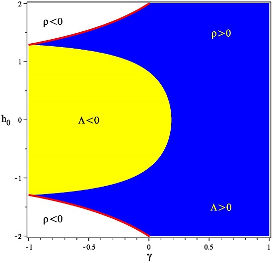
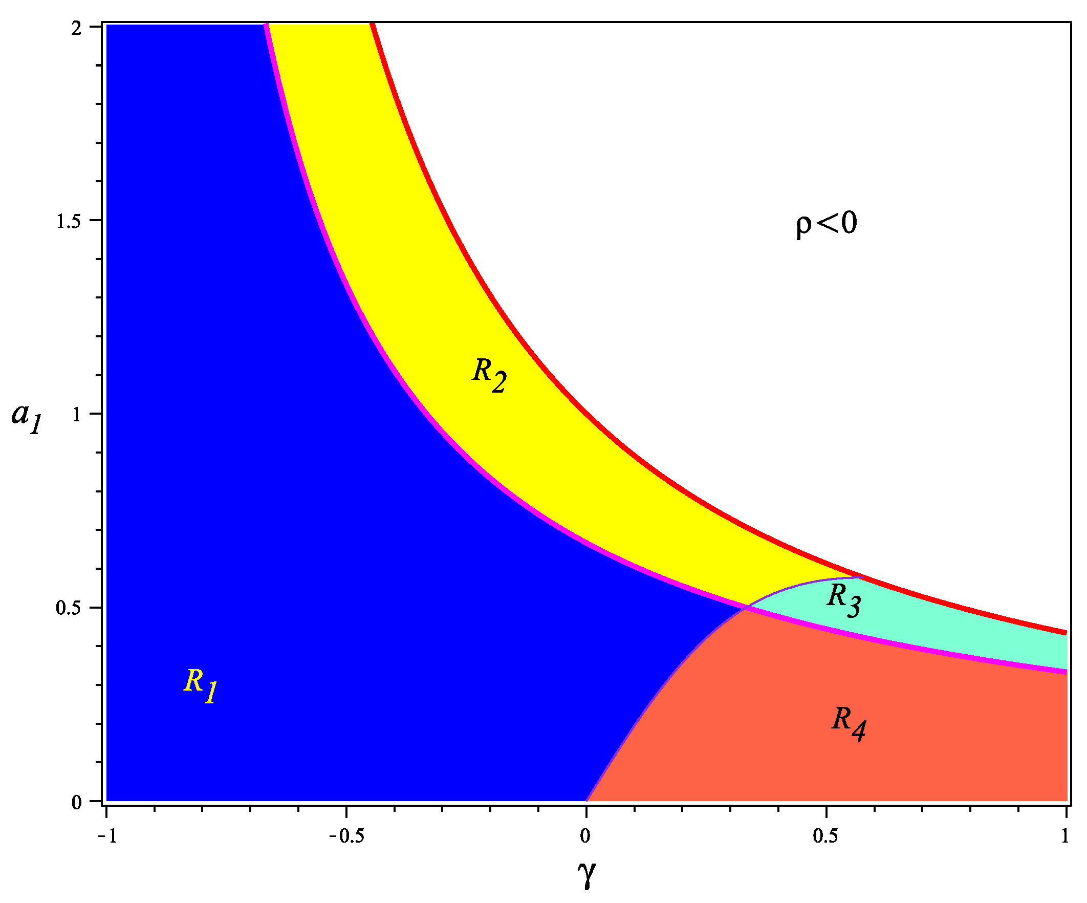
We study the case where the effective stress-energy tensor is defined by the matter field coupled to the dilaton and its potential, i.e., ${}^{\mathrm{eff}}{T}_{\mu \nu }={}^{(m)}{T}_{\mu \nu }+{}^{(\varphi )}{T}_{\mu \nu }+{}^{(V)}{T}_{\mu \nu }$. The solution found is the following one:

$$\begin{array}{cc}\hfill a& =t^{a_1},\varphi =\left(3a_1\left(\gamma +1\right)-2\right)lnt={\varphi }_{0}lnt\hfill \\ \hfill \Lambda & =\frac{\left(a_1\left(3{\gamma }^2+1\right)-2\gamma \right)\left(3a_1\left(\gamma +1\right)-2\right)}{\gamma +1}\hfill \\ \hfill {\rho }_0& =-\frac{3a_1^2\left(\gamma +1\right)+a_1\left(3\gamma -1\right)-2}{\gamma +1}\hfill \end{array}$$

(72)

We observe that all of the parameters depend on $\left(\gamma ,a_1\right)$. In order to analyze the solution, we assume that $\gamma \in \left(-1,1\right)$ and $a_1\in \left(0,2\right)$, since we are only interested in the case $t\in {\mathbb{R}}^{+}.$ In the figure (see Figure 1) we have plotted the region $\mathcal{R}$ of the space $\left(\gamma ,a_1\right)$ where the energy density is positive (the colored region). The red line stands for the border of this region, that is the set of points of $\left(\gamma ,a_1\right)$ where ${\rho }_0=0$, outside of $\mathcal{R}$, ${\rho }_0<0$; and therefore, the solution lacks any physical meaning. Inside of $\mathcal{R},$ we have marked four subregions, such that $\mathcal{R}={\cup }_{i=1}^4{\mathcal{R}}_i$ (see Figure 1). In the following table, we describe the behavior of each quantity in each subregion ${\mathcal{R}}_i$:

$$\begin{array}{|cccc|}\hline & \rho & \varphi & V\\ {\mathcal{R}}_1& >0& <0& <0\\ {\mathcal{R}}_2& >0& >0& >0\\ {\mathcal{R}}_3& >0& >0& <0\\ {\mathcal{R}}_4& >0& <0& >0\\ \hline\end{array}$$

(73)

Thus, subregions of physical interest are those where $\varphi <0,$ in order to get $e^{\varphi }$ bounded, which correspond to ${\mathcal{R}}_1$ and ${\mathcal{R}}_4$, noting furthermore that in ${\mathcal{R}}_4$, we have obtained $\Lambda >0.$ We see that when $a_1>1,$ the solution is inflationary, since the deceleration parameter, $q=a_1^{-1}-1<0,$ but if $a_1<1,$ then the solution is not inflationary. Therefore, we may find a set of values for the free parameters $\left(\gamma ,a_1\right)$, such that ${\rho }_0>0,$ $\Lambda >0$ and ${\varphi }_0<0,$ in such a way that $e^{\varphi }$ is bounded.

As an example, if we set $a_1=0.6$, then we find that ${\rho }_0=0$, if $\gamma =0.527$; therefore, the solution is only valid in the interval: $\gamma \in (-1,0,527)=I$. In this interval I, we find that the parameters Λ and ${\varphi }_0$ vanish at $\gamma =0.1$; thus Λ and ${\varphi }_0$ are negative if $\gamma \in (-1,0.1)$ and positive if $\gamma \in (0.1,0.527)$. To end, we note that $q>0$, since $a_1=0.6$.

(7)

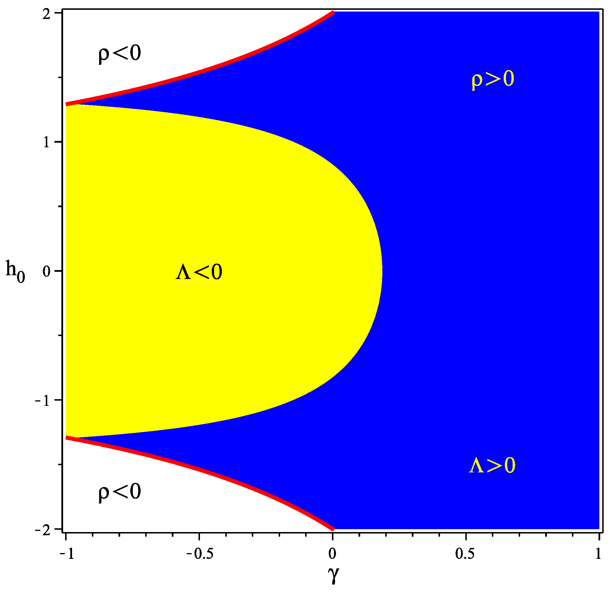
In the last model, we consider, ${}^{\mathrm{eff}}{T}_{\mu \nu }={}^{(m)}{T}_{\mu \nu }+{}^{(\varphi )}{T}_{\mu \nu }+{}^{(\mathbf{H})}{T}_{\mu \nu }+{}^{(V)}{T}_{\mu \nu },$ finding the following solution:

$$\begin{array}{cc}\hfill a_1& =\frac{1}{3},{\varphi }_0=\gamma -1,h_0=h_0\hfill \\ \hfill \Lambda & =\frac{\left(1-\gamma \right)\left(2\left(-3{\gamma }^2+6\gamma -1\right)+3h_0^2{\left(\gamma -1\right)}^2\right)}{6\left(\gamma +1\right)}\hfill \\ \hfill {\rho }_0& =-\frac{3h_0^2{\left(\gamma -1\right)}^2+8\gamma -12}{6\left(\gamma +1\right)}\hfill \end{array}$$

(74)

As is observed, since we are taking into account the $\mathbf{H}$-field, then we have obtained that the parameter of the scale factor is: $a_1=1/3$. As in the above model, we have plotted the region $\left(\mathcal{R}\right)$ of the space $(\gamma ,h_0)$ (the space of free parameters) where the energy density is positive (the colored region in Figure 2) and inside of $\mathcal{R}$ have marked in yellow color the set of points, such that $\Lambda <0$ (see Figure 2). We have assumed $\gamma \in (-1,1)$ and $h_0\in (-2,2)$. The red line stands for the border of $\mathcal{R}$, that is the set of values of the free parameters $(\gamma ,h_0)$ where ${\rho }_0=0$. As is observed, ${\varphi }_0<0$, for all $\gamma \in (-1,1),$ in such a way that the function $e^{\varphi }$ is bounded at late times, but the solution is not inflationary, $q>0$, since $a_1=1/3$.

Figure 1. FRW model described by: ${}^{\mathrm{eff}}{T}_{\mu \nu }=T_{\mu \nu }+{}^{(\varphi )}{T}_{\mu \nu }+{}^{(V)}{T}_{\mu \nu }.$ Plot of the region $\mathcal{R}$ (colored area), where the energy density is positive, $\gamma \in (-1,1]$ and $a_1\in (0,2]$. See (73) for an explanation of the subregions ${\mathcal{R}}_i$.

Figure 1. FRW model described by: ${}^{\mathrm{eff}}{T}_{\mu \nu }=T_{\mu \nu }+{}^{(\varphi )}{T}_{\mu \nu }+{}^{(V)}{T}_{\mu \nu }.$ Plot of the region $\mathcal{R}$ (colored area), where the energy density is positive, $\gamma \in (-1,1]$ and $a_1\in (0,2]$. See (73) for an explanation of the subregions ${\mathcal{R}}_i$.

Figure 2. FRW model with ${}^{\mathrm{eff}}{T}_{\mu \nu }={}^{(m)}{T}_{\mu \nu }+{}^{(\varphi )}{T}_{\mu \nu }+{}^{(\mathrm{H})}{T}_{\mu \nu }+{}^{(V)}{T}_{\mu \nu }$. Plot of the region $\mathcal{R}$ (colored area) where ${\rho }_0>0$ where $\gamma \in (-1,1]$ and $h_0\in [-2,2]$. Yellow color means $\Lambda <0$, while in the blue area, $\Lambda >0.$

Figure 2. FRW model with ${}^{\mathrm{eff}}{T}_{\mu \nu }={}^{(m)}{T}_{\mu \nu }+{}^{(\varphi )}{T}_{\mu \nu }+{}^{(\mathrm{H})}{T}_{\mu \nu }+{}^{(V)}{T}_{\mu \nu }$. Plot of the region $\mathcal{R}$ (colored area) where ${\rho }_0>0$ where $\gamma \in (-1,1]$ and $h_0\in [-2,2]$. Yellow color means $\Lambda <0$, while in the blue area, $\Lambda >0.$

5.2. Models with a Bianchi Type II Metric

A Bianchi Type II ($\mathrm{BII}$) metric is defined by (see [36] for details):

$$d{s}^2=-d{t}^2+a^2(t)d{x}^2+\left(b^2(t)+K^2{z}^2{a}^2(t)\right)d{y}^2+2K{a}^2(t)zdxdy+d^2(t)d{z}^2$$

(75)

where the scale factors ($a(t),b(t),d(t)$) are functions on time t and $K\in \mathbb{R}$. If $K=0,$ then the metric collapses to a Bianchi Type I ($\mathrm{BI})$ metric. We emphasize that in order to obtain self-similar solutions, the scale factors must behave as $a(t)=t^{a_1},$ $b(t)=t^{a_2},$ $d(t)=t^{a_3},$ and the parameters of the scale factors must verify the following relationship: $a_2+a_3=1+a_1$ (see [36,42]).

The FE for Metric (75) are as follows:

$$\begin{array}{cc}\hfill \frac{a^{\prime }}{a}\frac{b^{\prime }}{b}+\frac{a^{\prime }}{a}\frac{d^{\prime }}{d}+\frac{d^{\prime }}{d}\frac{b^{\prime }}{b}-\frac{K^2}{4}\frac{a^2}{b^2{d}^2}& =e^{\varphi }\rho +{\varphi }_t\theta -\frac{1}{2}{\varphi }_t^2+\frac{1}{4}{e}^{2\varphi }{h}_t^2+\frac{1}{2}V\hfill \end{array}$$

(76)

$$\begin{array}{cc}\hfill \frac{b^{″}}{b}+\frac{d^{″}}{d}+\frac{d^{\prime }}{d}\frac{b^{\prime }}{b}-\frac{3K^2}{4}\frac{a^2}{b^2{d}^2}& =-e^{\varphi }p+{\varphi }_{tt}+\left(\frac{d^{\prime }}{d}+\frac{b^{\prime }}{b}\right){\varphi }_t-\frac{1}{2}{\varphi }_t^2-\frac{1}{4}{e}^{2\varphi }{h}_t^2+\frac{1}{2}V\hfill \end{array}$$

(77)

$$\begin{array}{cc}\hfill \frac{K^2{a}^2}{b^2{d}^2}-\frac{b^{″}}{b}-\frac{d^{\prime }}{d}\frac{b^{\prime }}{b}+\frac{a^{″}}{a}+\frac{a^{\prime }}{a}\frac{d^{\prime }}{d}& =\left(\frac{a^{\prime }}{a}-\frac{b^{\prime }}{b}\right){\varphi }_t\hfill \end{array}$$

(78)

$$\begin{array}{cc}\hfill \frac{d^{″}}{d}+\frac{a^{″}}{a}+\frac{a^{\prime }}{a}\frac{d^{\prime }}{d}+\frac{K^2}{4}\frac{a^2}{b^2{d}^2}& =-e^{\varphi }p+{\varphi }_{tt}+\left(\frac{d^{\prime }}{d}+\frac{a^{\prime }}{a}\right){\varphi }_t-\frac{1}{2}{\varphi }_t^2-\frac{1}{4}{e}^{2\varphi }{h}_t^2+\frac{1}{2}V\hfill \end{array}$$

(79)

$$\begin{array}{cc}\hfill \frac{b^{″}}{b}+\frac{a^{″}}{a}+\frac{a^{\prime }}{a}\frac{b^{\prime }}{b}+\frac{K^2}{4}\frac{a^2}{b^2{d}^2}& =-e^{\varphi }p+{\varphi }_{tt}+\left(\frac{a^{\prime }}{a}+\frac{b^{\prime }}{b}\right){\varphi }_t-\frac{1}{2}{\varphi }_t^2-\frac{1}{4}{e}^{2\varphi }{h}_t^2+\frac{1}{2}V\hfill \end{array}$$

(80)

and the conservation equations:

$$\begin{array}{cc}\hfill h_{tt}+h_t\left(\theta +{\varphi }_t\right)& =0,\theta =\left(\frac{a^{\prime }}{a}+\frac{b^{\prime }}{b}+\frac{d^{\prime }}{d}\right)\hfill \end{array}$$

(81)

$$\begin{array}{cc}\hfill 2{\varphi }_{tt}+2\theta {\varphi }_t-{\varphi }_t^2-R+V-{\partial }_{\varphi }V+\frac{1}{2}{e}^{2\varphi }{h}_t^2& =0\text{or}\hfill \end{array}$$

(82)

$$\begin{array}{cc}\hfill {\varphi }_{tt}+\theta {\varphi }_t-{\varphi }_t^2+V+{\partial }_{\varphi }V-e^{2\varphi }{h}_t^2+e^{\varphi }\left(\rho +3p\right)& =0\hfill \end{array}$$

(83)

where:

$$R=2\left(\frac{a^{″}}{a}+\frac{b^{″}}{b}+\frac{d^{″}}{d}+\frac{a^{\prime }}{a}\frac{b^{\prime }}{b}+\frac{a^{\prime }}{a}\frac{d^{\prime }}{d}+\frac{d^{\prime }}{d}\frac{b^{\prime }}{b}-\frac{1}{4}\frac{a^2{K}^2}{b^2{d}^2}\right)$$

(84)

and the matter conservation equation:

$${\rho }^{\prime }+\left(1+\gamma \right)\rho \theta =0$$

(85)

with $\theta =u_{;\mu }^{\mu },$ $u^{\mu }=(1,0,0,0).$ We recall that the physical quantities must behave as follows:

$$\rho ={\rho }_0{t}^{-\left({\varphi }_0+2\right)},\varphi ={\varphi }_{0}lnt,h=h_0{t}^{-{\varphi }_0},V=C_1{e}^{-\frac{2}{{\varphi }_0}\varphi }$$

(86)

We go next to study the same models as the studied ones for the FRW metric, finding the following solutions.

(1)

In the first of the models, that is ${}^{\mathrm{eff}}{T}_{\mu \nu }={}^{(\varphi )}{T}_{\mu \nu },$ we have found the next solutions:

i

Under the self-similar condition (SSC) $a_2+a_3=1+a_1,$ we have obtained:

$$\begin{array}{cc}\hfill K& =0,\hfill \\ \hfill a_2& =\frac{1}{2}\left(1+a_1+\sqrt{-\left(a_1+1\right)\left(3a_1-1\right)}\right),\hfill \end{array}$$

(87)

$$\begin{array}{cc}\hfill a_3& =\frac{1}{2}\left(1+a_1-\sqrt{-\left(a_1+1\right)\left(3a_1-1\right)}\right),\hfill \\ \hfill {\varphi }_0& =2a_1\hfill \end{array}$$

As is observed, this solutions belongs to the BIclass, i.e., there is no solution Type BII. Note that:

$$\sum a_i=2a_1+1={\varphi }_0+1,q=\frac{-2\left(a_1-1\right)}{2a_1+1}$$

so the solution is inflationary iff $a_1>1$, but $e^{\varphi }$ is unbounded ($t\in {\mathbb{R}}^{+}$).

ii

Since the above solution is not of Type BII, we relax the hypothesis of self-similarity and try to find a power-law solution, finding in this case:

$$\begin{array}{cc}\hfill K& =0,\hfill \\ \hfill a_2& =\frac{1}{2}\left(1-a_1+{\varphi }_0+\sqrt{-3a_1^2+2a_1+2{\varphi }_0{a}_1+1-2{\varphi }_0-{\varphi }_0^2}\right),\hfill \\ \hfill a_3& =\frac{1}{2}\left(1-a_1+{\varphi }_0-\sqrt{-3a_1^2+2a_1+2{\varphi }_0{a}_1+1-2{\varphi }_0-{\varphi }_0^2}\right)\hfill \end{array}$$

(88)

which is of type BI. Note that if ${\varphi }_0=2a_1,$ then we recover the above solution. Therefore, there are no solutions of Type BII.

(2)

In the second model, described by: ${}^{\mathrm{eff}}{T}_{\mu \nu }={}^{(\varphi )}{T}_{\mu \nu }+{}^{(V)}{T}_{\mu \nu },$ we have obtained the following solutions:

i

By considering the SSC, $a_2+a_3=1+a_1,$ we get two solutions:

• The first of them is of type FRW:

  $$a_1=a_2=a_3=1,K=0,\Lambda ={\varphi }_0=1$$

  (89)
• The second one is given by (Type BII):

  $$\begin{array}{c}{a}_2=a_3=\frac{1}{2}\left(a_1+1\right),K^2=\frac{-\left(a_1-1\right)\left(3a_1-1\right)\left(a_1+1\right)}{5+3a_1},\hfill \\ \Lambda =\frac{\left(a_1+1\right)\left(3a_1-1\right){\left(3a_1+1\right)}^2}{{\left(5+3a_1\right)}^2},{\varphi }_0=\frac{6a_1+2}{5+3a_1}\hfill \end{array}$$

  (90)
  As we may observed, all of the parameters are positive ($a_1>0,$ when $t\in {\mathbb{R}}^{+}$); thus, the function $e^{\varphi }$ is unbounded at late times ($t\in {\mathbb{R}}^{+}$), and therefore, the solution has a limited physical interest.

ii

If we work without the SSC, then we get an FRW-like solution, i.e.,

$$K=0,a_1=a_2=a_3,{\varphi }_0=\frac{2a_1}{a_1+1},\Lambda =\frac{2a_1^2\left(3a_1^2-1\right)}{{\left(5+3a_1\right)}^2}$$

(91)

which lacks any physical interest.

(3)

When, ${}^{\mathrm{eff}}{T}_{\mu \nu }={}^{(\varphi )}{T}_{\mu \nu }+{}^{(\mathbf{H})}{T}_{\mu \nu },$ we get:

(a)

Under the SSC, we have obtained the following unphysical solution:

$$a_1=0,a_2=a_3=\frac{1}{2}={\varphi }_{0}h=i\in \mathbb{C},K=\frac{1}{2}i\in \mathbb{C}$$

(92)

note that $a_1=0$, so there is no BII solution for this model.

(b)

If we do not consider the SSC, then the obtained solution coincides with the obtained one in the case of the FRW model.

(4)

If ${}^{\mathrm{eff}}{T}_{\mu \nu }={}^{(\varphi )}{T}_{\mu \nu }+{}^{(\mathbf{H})}{T}_{\mu \nu }+{}^{(V)}{T}_{\mu \nu },$ we find that working under SSC, the solution lacks any physical interest, since:

$$a_1=0,a_2=a_3=\frac{1}{2},\Lambda ={\varphi }_0\left({\varphi }_0-\frac{2}{3}\right),K=\sqrt{-\frac{{\varphi }_0}{2}},h=\frac{1}{{\varphi }_0}\sqrt{1-\frac{5}{2}{\varphi }_0}$$

(93)

note that $a_1=0.$

If we try to find a power-law solution, then we obtain an FRW-like solution given by:

$$a=t^{1/3},\varphi ={\varphi }_{0}lnt,h=\frac{2\sqrt{3-6{\varphi }_0}}{3{\varphi }_0},\Lambda ={\varphi }_0\left({\varphi }_0-\frac{2}{3}\right)$$

(94)

with $a_1=a_2=a_3=\frac{1}{3}$ and ${\varphi }_0<\frac{1}{2}$, such that $V>0⟺{\varphi }_0<0.$ Note that this is the same solution as the obtained one working with the FRW metric. Therefore, there is no BII solution for this model.

(5)

In the model described by ${}^{\mathrm{eff}}{T}_{\mu \nu }={}^{(m)}{T}_{\mu \nu }+{}^{(\varphi )}{T}_{\mu \nu }+{}^{(\mathbf{H})}{T}_{\mu \nu },$ we have obtained the following solutions. The first of them, obtained under the SSC, has no physical meaning, since $a_1=0,$ while the rest of the permeates behave as follows:

$$a_2=a_3=\frac{1}{2},K=\sqrt{\frac{1}{2}\left(1-\gamma \right)},h=\frac{\sqrt{\frac{1}{2}\left(1-7\gamma +4{\gamma }^2\right)}}{\left(1-\gamma \right)},{\rho }_0=\frac{3}{2}-\gamma$$

(95)

If we do not consider the SSC, then we get an FRW-like solution. Therefore, there is no BII solution for this model.

(6)

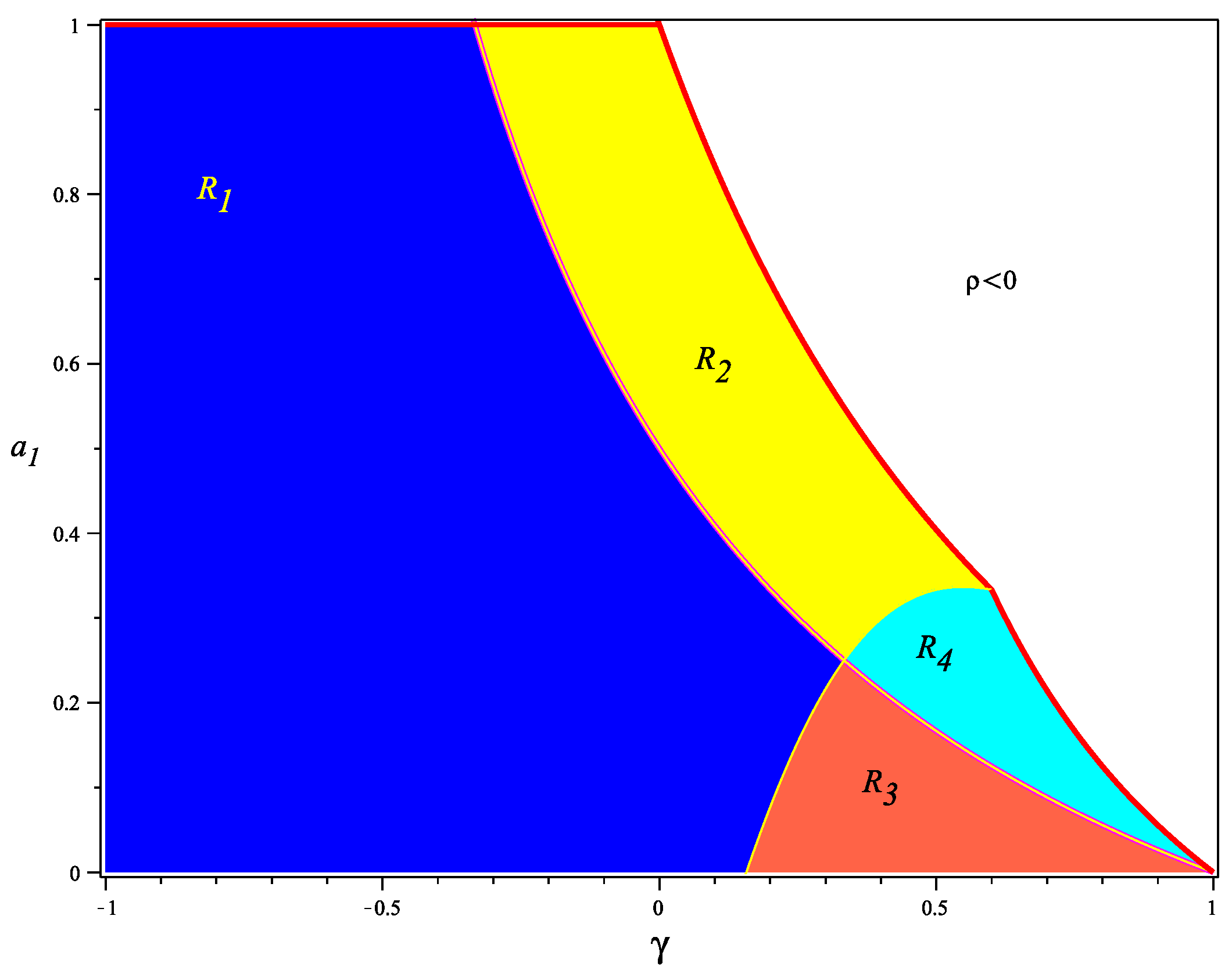
In this model, the effective stress-energy tensor takes the following form: ${}^{\mathrm{eff}}{T}_{\mu \nu }={}^{(m)}{T}_{\mu \nu }+{}^{(\varphi )}{T}_{\mu \nu }+{}^{(V)}{T}_{\mu \nu },$ obtaining a unique solution of type BII, which is self-similar:

$$\begin{array}{cc}\hfill K^2& =\frac{1}{2}\left(a_1-1\right)\left(\gamma \left(2a_1+1\right)-1\right),\hfill \\ \hfill a_2& =a_3=\frac{1}{2}\left(a_1+1\right),\hfill \\ \hfill {\varphi }_0& =2a_1\left(\gamma +1\right)+\gamma -1,\hfill \\ \hfill {\rho }_0& =\frac{7-a_1-5\gamma -13a_1\gamma -6a_1^2\left(\gamma +1\right)}{4\left(\gamma +1\right)},\hfill \\ \hfill \Lambda & =\frac{4{\left(2a_1+1\right)}^2{\gamma }^3+\left(2a_1+1\right)\left(7a_1-11\right){\gamma }^2+4\left(a_1^2-2a_1+2\right)\gamma +6a_1^2-a_1-1}{4\left(\gamma +1\right)}\hfill \end{array}$$

(96)

In Figure 3, we have plotted the region $\left(\mathcal{R}\right)$ of the space $\left(\gamma ,a_1\right)$ where the energy density is positive and $K^2$ is defined (the colored area under the red line). The red line stands for the border of this region, that is the set of points of $\left(\gamma ,a_1\right)$ where ${\rho }_0=0$ and $K^2=0$, and therefore, the solution does not belong to the Class BII. Outside of $\mathcal{R}$, ${\rho }_0<0$, and therefore, the solution lacks any physical meaning. Inside of $\mathcal{R},$ we have marked four subregions, such that $\mathcal{R}={\cup }_{i=1}^4{\mathcal{R}}_i$ (see Figure 3). In the following table, we describe the behavior of each quantity in each subregion ${\mathcal{R}}_i$:

$$\begin{array}{|cccc|}\hline & \rho & \varphi & V\\ {\mathcal{R}}_1& >0& <0& <0\\ {\mathcal{R}}_2& >0& >0& >0\\ {\mathcal{R}}_3& >0& <0& >0\\ {\mathcal{R}}_4& >0& >0& <0\\ \hline\end{array}$$

(97)

As we may see, we have a very similar plot as the obtained one for the FRW metric (see Figure (Figure 1)). Therefore, we may find values for the free parameters $\left(\gamma ,a_1\right),$ such that ${\rho }_0>0,$ ${\varphi }_0<0$ (in this way, $e^{\varphi }$ is bounded) and $\Lambda >0,$ obtaining a solution in agreement with the observations, but which is not inflationary, since $q=2(1-a_1)/(2a_1+1)>0,$ $\forall a_1<1$.

(7)

For the last of the studied models, ${}^{\mathrm{eff}}{T}_{\mu \nu }={}^{(m)}{T}_{\mu \nu }+{}^{(\varphi )}{T}_{\mu \nu }+{}^{(\mathbf{H})}{T}_{\mu \nu }+{}^{(V)}{T}_{\mu \nu },$ we have found a unique solutions, which is the same as the obtained one for the FRW metric; thus, there is no BII solution for this model.

Figure 3. Bianchi II model (BII) with an effective stress-energy tensor defined by: ${}^{\mathrm{eff}}{T}_{\mu \nu }=T_{\mu \nu }+{}^{(\varphi )}{T}_{\mu \nu }+{}^{(V)}{T}_{\mu \nu }$. Plot of the region $\mathcal{R}$ where the energy density is positive ${\rho }_0>0$ and $K^2>0$ (colored area), with $\gamma \in (-1,1]$ and $a_1\in (0,1]$. See (97) for an interpretation.

Figure 3. Bianchi II model (BII) with an effective stress-energy tensor defined by: ${}^{\mathrm{eff}}{T}_{\mu \nu }=T_{\mu \nu }+{}^{(\varphi )}{T}_{\mu \nu }+{}^{(V)}{T}_{\mu \nu }$. Plot of the region $\mathcal{R}$ where the energy density is positive ${\rho }_0>0$ and $K^2>0$ (colored area), with $\gamma \in (-1,1]$ and $a_1\in (0,1]$. See (97) for an interpretation.

6. Noether Symmetry Approach

In this section, we show how to reach similar results by using the method of the Noether symmetries [14], that is we are interested in determining the form of the physical quantities by employing this tactic, and if it is possible, then to obtain a complete solution of the resulting field equations. Due to the complexity of the method, we only study a particular case by taking into account the dilaton ϕ and the potential $V.$ Therefore, by taking into account the following action:

$$S=\frac{1}{2{\kappa }^2}\int d^{4}x\sqrt{-g}{e}^{-\varphi }\left[R+{\left(\nabla \varphi \right)}^2-V\right]$$

(98)

and the usual flat FRW metric given by Equation (56), so $R=6\left(H^2+a^{″}/a\right),$ we find that the model is described by the Lagrangian, with $Q=\left(a,\varphi \right)$ and $TQ=\left(a,\dot{a},\varphi ,\dot{\varphi }\right)$:

$$\mathcal{L}=e^{-\varphi }\left(6a{\dot{a}}^2+a^3\left({\varphi }_t^2+V\right)-6a^2\dot{a}{\varphi }_t\right)$$

(99)

where we note that the Hessian determinant $∥{\partial }_{{\dot{q}}_i{\dot{q}}_j}\mathcal{L}∥\ne 0.$ Therefore, the Euler–Lagrange equations yield (as we already know):

$$\begin{array}{c}2H^{\prime }+3H^2={\varphi }_{tt}+2H{\varphi }_t-\frac{1}{2}{\varphi }_t^2+\frac{1}{2}V(\varphi )\end{array}$$

(100)

$$\begin{array}{c}2{\varphi }_{tt}+6H{\varphi }_t-{\varphi }_t^2-R+V-{\partial }_{\varphi }V=0\end{array}$$

(101)

where $H=a^{\prime }/a,$ and the first FE is equivalent to:

$${\theta }_{\mathcal{L}}=\dot{a}{\partial }_{\dot{a}}\mathcal{L}+\dot{\varphi }{\partial }_{\dot{\varphi }}\mathcal{L}-\mathcal{L}=0$$

(102)

that is

$$3H^2=-\frac{1}{2}{\varphi }_t^2+3H{\varphi }_t+\frac{1}{2}V(\varphi )$$

(103)

The infinitesimal generator of the Noether symmetry, i.e., the lift vector X is now written as:

$$X=\alpha \frac{\partial }{\partial a}+\beta \frac{\partial }{\partial \varphi }+\frac{d\alpha }{dt}\frac{\partial }{\partial \dot{a}}+\frac{d\beta }{dt}\frac{\partial }{\partial \dot{\varphi }}$$

(104)

where $\alpha ,\beta$ are functions of a and ϕ and where:

$$\frac{d\alpha }{dt}=\dot{\alpha }=\left(\dot{a}\frac{\partial \alpha }{\partial a}+\dot{\varphi }\frac{\partial \alpha }{\partial \varphi }\right),\frac{d\beta }{dt}=\dot{\beta }=\left(\dot{a}\frac{\partial \beta }{\partial a}+\dot{\varphi }\frac{\partial \beta }{\partial \varphi }\right)$$

The existence of the Noether symmetry implies the existence of a vector field X, such that:

$$L_X\mathcal{L}=0$$

(105)

where $L_X$ stands for Lie derivative with respect to $X.$ If we calculate $L_X\mathcal{L}=0,$ then it yields (after simplifications):

$$\begin{array}{cc}\hfill \alpha -a\beta +2a\frac{\partial \alpha }{\partial a}-a^2\frac{\partial \beta }{\partial a}& =0\hfill \end{array}$$

(106)

$$\begin{array}{cc}\hfill 3\alpha -a\beta -6\frac{\partial \alpha }{\partial \varphi }+2a\frac{\partial \beta }{\partial \varphi }& =0\hfill \end{array}$$

(107)

$$\begin{array}{cc}\hfill -6\alpha +3a\beta -3a\frac{\partial \alpha }{\partial a}+6\frac{\partial \alpha }{\partial \varphi }+a^2\frac{\partial \beta }{\partial a}-3a\frac{\partial \beta }{\partial \varphi }& =0\hfill \end{array}$$

(108)

$$\begin{array}{cc}\hfill \left(3\alpha -a\beta \right)V+a\beta V^{\prime }& =0\hfill \end{array}$$

(109)

obtaining the following solutions:

(1)

Sol1:

$$\alpha =C_{1}a,\beta =3C_1,V=V_0$$

(110)

(2)

Sol2:

$$\alpha =C_1{a}^n{e}^{\varphi /2},\beta =\frac{-3}{n-1}{C}_1{a}^{n-1}{e}^{\varphi /2},V=V_0{e}^{n\varphi },n=(\sqrt{3}-1)/2$$

(111)

or:

$$\alpha =C_2{a}^m{e}^{\varphi /2},\beta =\frac{-3}{m-1}{C}_2{a}^{m-1}{e}^{\varphi /2},V=V_0{e}^{m\varphi },m=-(\sqrt{3}+1)/2$$

(112)

so $V=V_0{e}^{n\varphi },$ as we have obtained in the paper through different methods.

(3)

Sol3

$$\begin{array}{cc}\hfill \alpha & =C_{3}a+\left(C_1{a}^{(\sqrt{3}-1)/2}+C_2{a}^{(-\sqrt{3}-1)/2}\right)e^{\varphi /2},\hfill \\ \hfill \beta & =3C_3+\left(\left(\sqrt{3}+3\right)C_1{a}^{(\sqrt{3}-3)/2}+\left(3-\sqrt{3}\right)C_2{a}^{(-\sqrt{3}-3)/2}\right)e^{\varphi /2},\hfill \\ \hfill V& =0\hfill \end{array}$$

(113)

Therefore, we have found three different symmetries, which lead us to three different cosmological scenarios with three potentials; constant, dynamical and vanishing.

We start by studying the solution Equation (112). Once we have calculated the symmetries, there are several ways to obtain a complete solution, i.e., to obtain the exact expression for the scale factor and the scalar function. The first of them consists of studying the conserved quantities, since the existence of the symmetry X gives us a constant of motion, via the Noether theorem. The constant of motion generated by Sol2 (Equation (112)) yields:

$$Q_2=i_{{\mathbf{X}}_2}{\theta }_{\mathcal{L}}=2\sqrt{3}{a}^{(\sqrt{3}+1)/2}{e}^{-\varphi /2}{C}_1\left(-\left(\sqrt{3}+3\right)\dot{a}+a{\varphi }_t\right)$$

(114)

where the Cartan one form is given by ${\theta }_{\mathcal{L}}={\partial }_{\dot{a}}\mathcal{L}da+{\partial }_{\dot{\varphi }}\mathcal{L}d\varphi .$ If, for example, we set $Q_2=0,$ then we get: $\varphi ={\varphi }_{0}lna.$ Thus, we see that the existence of the Noether symmetry allows us to determine a complete integration. In the same way (see, for instance, [43,44]), we may observe that from the equation:

$$L_X\mathcal{L}=\alpha {\partial }_a\mathcal{L}+\dot{\alpha }{\partial }_{\dot{a}}\mathcal{L}+\beta {\partial }_a\mathcal{L}+\dot{\beta }{\partial }_{\dot{\varphi }}\mathcal{L}=0$$

(115)

where ${\partial }_{\dot{a}}\mathcal{L}=p_a,$ and by taking into account the E-Lequations, then $L_X\mathcal{L}=0$ yields:

$$\frac{d}{dt}\left(\alpha p_a+\beta p_{\varphi }\right)=0$$

(116)

therefore, the conserved quantity yields: $Q=\alpha p_a+\beta p_{\varphi }$; so, in this case, we get:

$$\left(m-1\right)Q=6a^{m+1}{e}^{-\varphi /2}\left(\left(2m+1\right)\dot{a}-ma{\varphi }_t\right)$$

(117)

If we set $Q=0,$ then we obtain:

$$\varphi =\frac{\left(2m+1\right)}{m}lna,m=-(\sqrt{3}+1)/2,\varphi =\left(3-\sqrt{3}\right)lna$$

(118)

by introducing this result into Equation (103), we get $a(t)=t^{a_1},$ as is expected, and therefore, $\varphi ={\varphi }_{0}lnt$, which is the solution obtained through the matter collineation approach and the invariant solution obtained through the Lie group method. However, if $Q\ne 0,$ then:

$$\varphi =\frac{\left(2m+1\right)}{m}lna-\frac{2}{m}ln\left(\frac{\left(m-1\right)Q}{12m}\left(t+c_1\right)\right)$$

(119)

and taking into account the first of the FE Equation (103), we get the following solution for the scale factor:

$$a(t)=2^{-\frac{2\sqrt{3}}{3}}{\left(4c_2{\left(t+c_1\right)}^{\sqrt{3}-1}+3\left(4\sqrt{3}+7\right)V_0\right)}^{\frac{\sqrt{3}}{3}}$$

(120)

As a final remark about the invariant solution, we can also consider that it is possible to find an invariant solution induced, for example, by:

$$\alpha =C_2{a}^m{e}^{\varphi /2},\beta =\frac{-3}{m-1}{C}_2{a}^{m-1}{e}^{\varphi /2},m=-(\sqrt{3}+1)/2$$

such that:

$$\frac{da}{\alpha }=\frac{d\varphi }{\beta }⟹\varphi =\frac{3}{1-m}lna=\left(3-\sqrt{3}\right)lna$$

(121)

which is the conserved quantity deduced previously. However, all of these solutions are particular solutions. Thus, in order to find the complete solution for the scalar function and the scale factor, we may consider the following method. We use X for finding a new set of variables, in such a way that in the new coordinates, the transformed Lagrangian is cyclic in one of them [14]. This is achieved iff, for $z=z(a,\varphi )$ and $w=w(a,\varphi ),$ $i_{\mathbf{X}}\left(dz\right)=1,$ $i_{\mathbf{X}}\left(dw\right)=0,$ with α and β given by Equation (112), finding, for example (there are several solutions, and not all of them work well), the following one:

$$w=\left(\sqrt{3}-3\right)lna+\varphi ,z=\frac{\sqrt{3}}{3}{a}^{\frac{1}{2}\left(3+\sqrt{3}\right)}{e}^{-\frac{1}{2}\varphi }$$

(122)

and therefore:

$$a=e^{\frac{\sqrt{3}}{6}w}{\left(\frac{\sqrt{3}}{z}\right)}^{-\frac{\sqrt{3}}{3}},\varphi =\frac{1}{2}\left(w\left(\sqrt{3}+1\right)+\left(\sqrt{3}-1\right)ln3+2\left(1-\sqrt{3}\right)ln\left(\frac{1}{z}\right)\right)$$

(123)

By rewriting the Lagrangian in the coordinates $\left(w,z\right)$, it yields:

$$\overline{\mathcal{L}}=-e^{-\frac{1}{2}w}\left(2\sqrt{3}\dot{z}\dot{w}+V_0{e}^{-\frac{1}{2}w\left(\sqrt{3}+2\right)}\right)$$

(124)

and therefore, the new E-L equations are:

$$\ddot{w}=\frac{{\dot{w}}^2}{2},\ddot{z}=\frac{1}{4}\left(1+\sqrt{3}\right)V_0{e}^{-\frac{1}{2}w\left(\sqrt{3}+2\right)}$$

(125)

finding in this way that:

$$w=-2ln\left(-\frac{1}{2}\left(c_{1}t+c_2\right)\right),c_1,c_2\in \mathbb{R}$$

(126)

and:

$$z=K{\left(c_{1}t+c_2\right)}^4{\left(-\frac{1}{2}\left(c_{1}t+c_2\right)\right)}^{\sqrt{3}}+c_{3}t+c_4$$

(127)

with $K=V_0\left(\sqrt{3}+1\right)\left(\sqrt{3}-3\right)\left(\sqrt{3}-4\right)/1248c_1^2.$ Now, we recover the solution in the original variables $\left(a,\varphi \right)$:

$$a=\frac{{\left(2\sqrt{3}\right)}^{\sqrt{3}/3}}{{\left(-c_{1}t-c_2\right)}^{\frac{1}{3}\sqrt{3}}}{\left(K{\left(c_{1}t+c_2\right)}^4{\left(-\frac{1}{2}\left(c_{1}t+c_2\right)\right)}^{\sqrt{3}}+c_{3}t+c_4\right)}^{\frac{\sqrt{3}}{3}}$$

(128)

$$\varphi =-ln\left(-\frac{1}{2}\left(c_{1}t+c_2\right)\right)\left(\sqrt{3}+1\right)+\left(1-\sqrt{3}\right)ln\left(\frac{1}{K{\left(c_{1}t+c_2\right)}^4{\left(-\frac{1}{2}\left(c_{1}t+c_2\right)\right)}^{\sqrt{3}}+c_{3}t+c_4}\right)+C_1$$

(129)

with $C_1=\left(\sqrt{3}-1\right)ln3.$ In order to get solutions with physical meaning, we need to impose the assumption ${\left(c_i\right)}_{i=1}^4$ $\le 0.$ In the following plots (Figure 4), we show the behavior of the scale factor $a(t)$, the deceleration parameter q and the dilaton field $\varphi (t).$ As we can see, the solution is inflationary, $q<1$, showing furthermore an acceleration expansion at late times, while the dilaton ($e^{\varphi }$) is unbounded, but the potential function is decreasing since $V=V_0{e}^{m\varphi },$ with $m=-(\sqrt{3}+1)/2<0.$ Compare this solution to the obtained one in Equation (68).

We would like to emphasize that for an adequate choice of the constants of integration, basically, we have obtained the following results:

$$a\approx a_0{t}^{a_1},\varphi \approx {\varphi }_{0}lnt,V=V_0{e}^{n\varphi },a_1,n\in \mathbb{R}$$

which is, in essence, the same result as the obtained one in the previous sections.

Figure 4. Plot of the quantities, $a(t),$ q and $\varphi (t).$ Numerical values of the constants: $c_1=-1,$ $c_2=-1,$ $c_3=-1/624$ and $c_4=0.$ Note that the solution is inflationary and has an accelerated expansion at late time without any transition to a decelerated era.

Figure 4. Plot of the quantities, $a(t),$ q and $\varphi (t).$ Numerical values of the constants: $c_1=-1,$ $c_2=-1,$ $c_3=-1/624$ and $c_4=0.$ Note that the solution is inflationary and has an accelerated expansion at late time without any transition to a decelerated era.

With regard to the first of the symmetries Equation (110), that is $\alpha =a,$ $\beta =3$ and $V=V_0,$ following the same steps as above, we find that $Q=\alpha p_a+\beta p_{\varphi }$; therefore, $-e^{-\varphi }6a^2\dot{a}=Q,$ finding in this way that:

$$a=\frac{1}{2}{\left(-4Q\int e^{\varphi }dt+8c_1\right)}^{1/3}$$

(130)

but we are not able to obtain more information. Now, if we calculate the cv, $z=z(a,\varphi )$ and $w=w(a,\varphi ),$ induced by the symmetry, we may find that: $w=-3lna,$ $z=lna$; so $a=e^z$ and $\varphi =w+3z.$ With these new variables, the Lagrangian yields:

$$\mathcal{L}=e^{-w}\left({\dot{w}}^2-3{\dot{z}}^2+V_0\right)$$

(131)

in such a way that the new EL equations are:

$$\begin{array}{ccc}\hfill \ddot{z}& =& \dot{w}\dot{z},\hfill \end{array}$$

(132)

$$\begin{array}{ccc}\hfill 2\ddot{w}& =& {\dot{w}}^2+3{\dot{z}}^2-V_0\hfill \end{array}$$

(133)

finding that

$$z=c_1+c_2\int e^{w}dt$$

(134)

where $c_1,c_2$ are constants of integration, but we are only able to find a particular solution for $w,$ $w=w_0,$ that is a constant. Calculating the inverse cv, we arrive at the following solution:

$$a=e^t,\varphi ={\varphi }_{0}t$$

(135)

thus, this particular solution is quite similar to the obtained one through the Lie group method with the symmetry $\left[a,1\right].$

7. Conclusions

We have studied how to find the functional form of the physical quantities, $V,$ $h,$ ϕ and $\rho ,$ of the low energy string-inspired cosmological models by using several symmetry methods. We have proven, through the matter collineation approach (MC), the exact form that each physical quantity must take in the string frame; see Theorem 1. Therefore, we have proven that there exist self-similar solutions (SS) and how each physical quantity must behave in order for the FE to admit such a kind of solution. In the same way, we have formalized the use of power-law solutions (less restrictive than the self-similar ones) by studying the wave equation for the dilaton through the Lie group method (LG); see Theorem 2. Since we have not been able to find the general solution of the wave equation, then we have obtained the invariant solution induced by the imposed symmetry. This invariant solution coincides with the SS one. We have shown that the LG method is a powerful method to obtain the functional form of the unknown functions. In this paper, we have been more interested in obtaining solutions similar to the SS ones, but by imposing other symmetries, we are able to obtain other integrable solutions, as we have shown. In this case, the obtained solution is always inflationary, $q=-1$, and it verifies the T-duality property for the scale factor, while the potential is constant, that is $V=V_0$.

As examples, we have calculated exact self-similar and power-law solutions to several string cosmological models by using two geometries, the FRW and the Bianchi Type II one. In these models, we have studied how each physical field affects the solution, that is we have studied several cosmological models in the four-dimensional NS-NSsector of low-energy effective string theory coupled to a dilaton and an axion-like $\mathbf{H}$-field within the string frame background; Cases (1)–(7).

In the FRW background, we have shown that, if we take into account the $\mathbf{H}$-field, then the solutions are quite restrictive, since in Case (3), where the effective stress-energy tensor is defined by ${}^{\mathrm{eff}}{T}_{\mu \nu }={}^{(\varphi )}{T}_{\mu \nu }+{}^{(\mathbf{H})}{T}_{\mu \nu },$ we obtained imaginary solutions, while in the rest of the cases studied, the h-equation, that is Equation (59), brings us to get $a_1=1/3,$ that is the exponent of the scale factor only takes this value. Nevertheless, we have obtained two solutions (see Cases (6 and 7)) that are interesting from the physical point of view, since in these cases, we have obtained ${\rho }_0>0,$ ${\varphi }_0<0$ (in this way, $e^{\varphi }$ is bounded) and $\Lambda >0.$ Furthermore, in Case (6), we may find values for the free parameters in such a way that the solution is also inflationary.

In the case of Bianchi Type II geometry, we have shown that there are only two self-similar solutions, which correspond to Cases (2) and (6), where Case (6) could be of particular physical interest, since in it, we found that the solution gives $e^{\varphi }$ bounded at late times, with Λ and ρ positive. The rest of the obtained solutions under the self-similar hypothesis are unphysical, since the exponent of the scale factor $a(t)=t^{a_1}$ is equal naught, $a_1=0$. Therefore, the self-similar condition is very restrictive. By working under the power-law hypothesis (less restrictive than the self-similar one), we have shown that all of the obtained solutions collapse to the obtained ones with the FRW geometry, except in Case (1), where the solution belongs to the Bianchi I class.

We have also studied the existence of Noether symmetries in the particular case of the FRW geometry, finding three symmetries with different potentials, constant, dynamical and vanishing. In the first of the studied cases, with a dynamical potential, we have shown that the conserved quantity induced by this symmetry brings us to obtain the same result as with the MC and LG (power-law solution) methods. However, in this case, we have been able to obtain a complete solution to the E-L equations through the change of variables method. This solution is inflationary and has an accelerated expansion at late times without any transition to a decelerated era, and for a suitable choice of the constants of integration, it may collapse to the obtained one through the previous symmetry methods, that is the MC and LG methods. In the second studied symmetry, we have shown that this solution (particular solution) is very similar to the obtained one through the LGM (second solution). This solution verifies the $T-$duality symmetry property and has a constant potential, and it is always inflationary, since the deceleration parameter $q=-1$. Nevertheless, this method has some drawbacks in comparison to the other ones. The Noether method is only applicable to one geometry (for example, FRW), while with the other tactics, we have been able to get general results valid for any Bianchi geometry and the FRW one; so, it is necessary to study case by case. Noether’s method also depends on many change of variables, but not all of them bring us to get correct solutions from the physical point of view. The matter collineation approach is maybe the simplest one, but as we have shown with the examples, not all of the self-similar solutions have physical meaning, since we have obtained some complex solutions (where the numerical constants belong to the complex numbers).

References

- Gasperini, M. Elements of String Cosmology; Cambridge University Press: Cambridge, UK, 2007. [Google Scholar]
- Lidsey, J.E.; Wands, D.; Copeland, E.J. Superstring Cosmology. Phys. Rep. 2000, 337, 343–492. [Google Scholar] [CrossRef]
- Duff, M.J. M-Theory (the Theory Formerly Known as Strings). Int. J. Mod. Phys. A 1996, 11, 5623–5642. [Google Scholar] [CrossRef]
- Copeland, E.J.; Lahiri, A.; Wands, D. Low energy effective string cosmology. Phys. Rev. D 1994, 50, 4868–4880. [Google Scholar] [CrossRef]
- Veneziano, G. Scale factor duality for classical and quantum strings. Phys. Lett. B 1991, 265, 287–294. [Google Scholar] [CrossRef]
- Ellis, G.F.R.; Roberts, D.C.; Solomons, D.; Dunsby, P.K.S. Solution to the graceful exit problem in pre-big bang cosmology. Phys. Rev. D 2000, 62, 084004. [Google Scholar] [CrossRef]
- Rosquist, K.; Jantzen, R. Spacetimes with a transitive similarity group. Class. Quant. Gravity 1985, 2, L129. [Google Scholar] [CrossRef]
- Coley, A.A. Dynamical Systems and Cosmology; Kluwer Academic: Dordrecht, The Netherlands, 2003. [Google Scholar]
- Carr, B.J.; Coley, A.A. Self-similarity in general relativity. Class. Quant. Gravity 1999, 16, R31–R71. [Google Scholar] [CrossRef]
- Ovsiannikov, L.V. Group Analysis of Differential Equations; Academic Press: New York, NY, USA, 1982. [Google Scholar]
- Nojiri, S.; Odintsov, S.D.; Sami, M. Dark energy cosmology from higher-order, string-inspired gravity and its reconstruction. Phys. Rev. D 2006, 74, 046004. [Google Scholar] [CrossRef]
- Elizalde, E.; Jhingan, S.; Nojiri, S.; Odintsov, S.D.; Sami, M.; Thongkool, I. Dark energy generated from a super)string effective action with higher order curvature corrections and a dynamical dilaton. Eur. Phys. J. C 2008, 53, 447–457. [Google Scholar] [CrossRef]
- De Ritis, R.; Marmo, G.; Platania, G.; Rubano, C.; Scudellaro, P.; Stornaiolo, C. New approach to find exact solutions for cosmological models with a scalar field. Phys. Rev. D 1990, 42, 1091–1097. [Google Scholar] [CrossRef]
- Capozziello, S.; De Laurentis, M.; Odintsov, S.D. Hamiltonian dynamics and Noether symmetries in Extended Gravity Cosmology. Eur. Phys. J. C 2012, 72, 1–21. [Google Scholar] [CrossRef]
- Kalotas, T.M.; Wybourne, B.G. Dynamical Noether symmetries. J. Phys. A Math. Gen. 1982, 15, 2077–2083. [Google Scholar] [CrossRef]
- Ibragimov, N.H. Elementary Lie Group Analysis and Ordinary Differential Equations; Wiley: New York, NY, USA, 1999. [Google Scholar]
- Terzis, P.A.; Dimakis, N.; Christodoulakis, T. Noether analysis of Scalar-Tensor Cosmology. Phys. Rev. D 2014, 90, 123543. [Google Scholar] [CrossRef]
- Christodoulakis, T.; Dimakis, N.; Terzis, P.A. Lie point and variational symmetries in minisuperspace Einstein’s gravity. J. Phys. A Math. Theor. 2014, 47, 095202. [Google Scholar] [CrossRef]
- Fradkin, E.S.; Tseytlin, A.A. Quantum string theory effective action. Nucl. Phys. B 1985, 261, 1–27. [Google Scholar] [CrossRef]
- Callan, C.G.; Martinec, E.J.; Perry, M.J.; Friedan, D. Strings in background fields. Nucl. Phys. B 1985, 262, 593–609. [Google Scholar] [CrossRef]
- Lovelace, C. Stability of string vacua: (I). A new picture of the renormalization group. Nucl. Phys. B 1985, 273, 413–467. [Google Scholar] [CrossRef]
- Green, M.B.; Schwarz, J.H.; Witten, E. Superstring Theory; Cambridge University Press: Cambridge, UK, 1987; Volume I–II. [Google Scholar]
- Polchinski, J. String Theory; Cambridge University Press: Cambridge, UK, 1998; Volume I–II. [Google Scholar]
- Johnson, C.V. D-Brane Primer. 2000; arXiv:hep-th/0007170. [Google Scholar]
- Candelas, P.; Horowitz, G.T.; Strominger, A.; Witten, E. Vacuum configurations for superstrings. Nucl. Phys. 1985, 258, 46–74. [Google Scholar] [CrossRef]
- Witten, E. Dimensional reduction of superstring models. Phys. Lett. B 1985, 155, 151–155. [Google Scholar] [CrossRef]
- Witten, E. New issues in manifolds of SU(3) holonomy. Nucl. Phys. B 1986, 268, 79–112. [Google Scholar] [CrossRef]
- Freund, P.G.O.; Rubin, M.A. Dynamics of dimensional reduction. Phys. Lett. B 1980, 97, 233–235. [Google Scholar] [CrossRef]
- Rosas-Lopez, I.C.; Kitazawa, Y. Antisymmetric field in string gas cosmology. Phys. Rev. D 2010, 82, 126005. [Google Scholar] [CrossRef]
- Tseytlin, A.A. Cosmological Solutions with dilaton and maximally symmetric space in string theory. Int. J. Mod. Phys. D 1992, 1, 223–245. [Google Scholar] [CrossRef]
- Goldwirth, D.S.; Perry, M.J. String-Dominated Cosmology. Phys. Rev. D 1994, 49, 5019–5025. [Google Scholar] [CrossRef]
- Belinchón, J.A. Generalized self-similar scalar-tensor theories. Eur. Phys. J. C 2012, 72, 1–16. [Google Scholar] [CrossRef]
- Cahill, M.E.; Taub, A.H. Spherically symmetric similarity solutions of the Einstein field equations for a perfect fluid. Commun. Math. Phys. 1971, 21, 1–40. [Google Scholar] [CrossRef]
- Eardley, D.M. Self-similar spacetimes: Geometry and dynamics. Commun. Math. Phys. 1974, 37, 287–309. [Google Scholar] [CrossRef]
- Hall, G. Symmetries and Curvature Structure in General Relativity; Lecture Notes in Physics; World Scientific: Singapore, 2004. [Google Scholar]
- Hsu, L.; Wainwright, J. Self-similar spatially homogeneous cosmologies: Orthogonal perfect fluid and vacuum solutions. Class. Quant. Gravity 1986, 3, 1105–1124. [Google Scholar] [CrossRef]
- Bluman, G.W.; Anco, S.C. Symmetry and Integration Methods for Differential Equations; Springer-Verlang: Berlin, Germany, 2002. [Google Scholar]
- Sheftel, M.B. Lie groups and differential equations: Symmetries, conservation laws and exact solutions of mathematical models in physics. Phys. Elem. Part. Fields 1997, 28, 241–266. [Google Scholar] [CrossRef]
- Veneziano, G. Inhomogeneous Pre-Big Bang String Cosmology. Phys. Lett. B 1997, 406, 297–303. [Google Scholar] [CrossRef]
- Barrow, J.D.; Kunze, K.E. String Cosmology. Chaos Solitons Fractals 1999, 10, 257–265. [Google Scholar] [CrossRef]
- Blaschke, D.B.; Dabrowski, M.P. Conformal relativity versus Brans–Dicke and superstring theories. Entropy 2012, 14, 1978–1996. [Google Scholar] [CrossRef]
- Belinchón, J.A. Bianchi II with time varying constants. Self-similar approach. Astrophys. Space Sci. 2009, 323, 185–195. [Google Scholar] [CrossRef]
- Vakili, B. A late time accelerated FRW model with scalar and vector fields via Noether symmetry. Phys. Lett. B 2014, 738, 488–492. [Google Scholar] [CrossRef]
- Zhang, S. On Noether approach in the cosmological model with scalar and gauge fields: Symmetries and the selection rule. 2015; arXiv:1504.04695. [Google Scholar]
© 2016 by the author; licensee MDPI, Basel, Switzerland. This article is an open access article distributed under the terms and conditions of the Creative Commons by Attribution (CC-BY) license (http://creativecommons.org/licenses/by/4.0/).
Share and Cite
MDPI and ACS Style
Belinchón, J.A. String-Inspired Gravity through Symmetries. Universe 2016, 2, 3. https://doi.org/10.3390/universe2010003
AMA Style
Belinchón JA. String-Inspired Gravity through Symmetries. Universe. 2016; 2(1):3. https://doi.org/10.3390/universe2010003
Chicago/Turabian StyleBelinchón, José Antonio. 2016. "String-Inspired Gravity through Symmetries" Universe 2, no. 1: 3. https://doi.org/10.3390/universe2010003
Note that from the first issue of 2016, this journal uses article numbers instead of page numbers. See further details here.