Coevolution of the Features of the Dynamics of the Accelerator Pedal and Hyperparameters of the Classifier for Emergency Braking Detection

Abstract

We investigate the feasibility of inferring the intention of the human driver of road motor vehicles to apply emergency braking solely by analyzing the dynamics of lifting the accelerator pedal. Focusing on building the system that reliably classifies the emergency braking situations, we employed evolutionary algorithms (EA) to coevolve both (i) the set of features that optimally characterize the movement of accelerator pedal and (ii) the values of the hyperparameters of the classifier. The experimental results demonstrate the superiority of the coevolutionary approach over the analogical approaches that rely on an a priori defined set of features and values of hyperparameters. By using simultaneous evolution of both features and hyperparameters, the learned classifier inferred the emergency braking situations in previously unforeseen dynamics of the accelerator pedal with an accuracy of about 95%. We consider the obtained results as a step towards the development of a brake-assisting system, which would perceive the dynamics of the accelerator pedal in a real-time and in case of a foreseen emergency braking situation, would apply the brakes automatically well before the human driver would have been able to apply them.

1. Introduction

In recent years, the technological growth of the intellectual driving aid cannot be overlooked [1]. The interest in this field is dictated by the needs of increasing the safety of the road traffic. Nearly 1.3 million people die in road crashes every year [2]. Part of these tragedies is caused by too-late brake application that could be prevented by embedding automated brake assistance into the cars. This type of assisting could be integrated either as a fully automated braking system [3,4] or as an assistant to the human driver [5,6]. The automated braking system is considered to be beneficial in many traffic situations. However, this type of aid suffers from serious engineering and psychological problems. One of these problems—according to risk homeostasis theory [7]—is overconfidence in the fully automated driving aids, which, in turn, could possibly blunt the human driver and lead to dangerous situations on the roads. The engineering problems include the reliability and validity of sensors. With an intention to create a safe system devoid of the mentioned drawbacks, we decided to leave the fully automated braking aids out of the scope of our research and focus on brake assistance instead. For implementing the brake assistance, the emergency braking classification (EBC) problem [8] must be solved.

The EBC problem can be addressed by different techniques, such as an analysis of the motion pattern of the pressed brake pedal [9], or measuring the brain and the myoelectric activities, as proposed in the research of Haufe et al. [10]. Another possible solution of the EBC problem could be based on the analysis of time series of the position of the accelerator pedal [11].

As shown in Figure 1, the specific motion of the accelerator pedal corresponds to a specific driving situation—such as accelerating, cruising, slowing down, normal braking, and emergency braking. A depicted time series of the position of both the accelerator- and brake pedals was obtained from the simulated parametric data recorder of the full-scale Forum-8 drive simulator [12], as shown in Figure 2.

In one of our previous studies [8] on the EBC problem, besides showing the possibility of distinguishing between normal driving and emergency braking situations solely by analyzing the motion of the accelerator pedal, we also demonstrated that straightforward approaches such as threshold classifiers were not feasible for the EBC problem, because of the impossibility of accurately separating the data set into two categories of normal driving and emergency braking, respectively. Under the same work, we revealed that during the emergency braking, the average time lag of a human driver is within the interval (200 ms, 400 ms). Consequently, for the speed of 72 km/h (20 m/s), an eventual EBS would reduce the overall braking distance by 4 to 8 m.

In our work [13] we proposed a method of applying genetic algorithms (GA) for (i) tuning the hyper-parameters and (ii) selecting the best combinations of manually extracted features of the time series of the accelerator pedal in order to increase the quality of classifiers. The classifier with the best-evolved values of hyper-parameters could distinguish normal driving from emergency braking situations with an accuracy of about 93%. Despite these results achieved by applying GA to the EBC problem, we considered the priority of further improvement of the classification quality and investigated the feasibility of employing a more versatile and flexible approach—cooperative coevolution—for the simultaneous optimization of both (i) the features of the time series of accelerator pedal, and (ii) the values of the hyperparameters of the classifier.

The evolutionary computation as a method for optimizing different classifiers has been explored in plenty of studies. Most frequently, among all evolutionary approaches, the researchers resort to genetic programming (GP) and GA. Thus, in one of the studies [14], the authors use the GP for extracting the features for epileptic electroencephalography (EEG) classification. They could successfully reduce the dimensionality of the feature space and improve the performance of the classifier. In another study [15], the authors employ GP to search for the set of mappings with optimal dimensionality to project the input space into a decision space with maximized class separability. Feature extraction by genetic programming was also successfully applied for vision systems [16]. The GA, on the other hand, has been widely used for searching for optimal values of the hyperparameters as an alternative to exhaustive (“brute-force”) searches. For example, Francescomarino et al. [17] employ the GA for hyperparameter optimization in predictive business process monitoring. Another good example of a successful application of the GA is the research of Ahmadi et al. [18], where the authors apply the GA for searching the optimal hyperparameters for least squares support vector machine.

Inspired by the success of the aforementioned research, we decided to employ cooperative coevolution for solving the EBC problem by the coevolution of both (i) the values of hyperparameters of the classifier and (ii) the features pertinent to the dynamics of accelerator pedal. The primary objective of our research is to verify the superiority of the coevolution over the other techniques that were considered in previous studies of EBC. We shall also examine the generality of the proposed solution to the EBC problem on the unforeseen data of human drivers who have not participated in obtaining the training set. The key motivation of our research is the exploration of the opportunity to significantly improve the quality of the classifier of EBC.

The latter would facilitate the reduction of the time lag between the following two instants: the instant the driver moves their foot away from the accelerator pedal (a in Figure 3) and the moment when they press the brake pedal to its maximum position (c in Figure 3). In properly classified cases, the proposed brake-assisting system would be able to activate the brakes automatically well before the human driver would have been able to apply them, and, as a consequence, to reduce the braking distance caused by the above-mentioned time lag.

The remaining of this article is organized as follows. Section 2 describes the methods that we used in our research. Section 3 outlines the proposed approach. In Section 4 we explain the research methodology. Section 5 presents the experimental results. Section 6 discusses the uncertainty of the evolved classifier. Finally, Section 7 draws a conclusions.

2. Methods

In our research we use the tools as explained below in this section.

2.1. Cooperative Coevolution

Cooperative coevolution (CC) [19,20] is a general framework of evolutionary computation that divides a large problem into subcomponents and solves them independently in order to solve the large problem. Like other evolutionary approaches, CC is characterized by the iterative improvement of the set of candidate solutions. Improvement implies the increase of fitness value through the selection, reproduction, and mutations of solutions. In CC, the candidate solutions are decomposed into smaller species that are evolved mostly separately, with the only cooperation happening during fitness evaluation. In our work we are focused on the application of CC for both: (i) automatic extraction of features pertinent to the time series of the position of accelerator pedal and (ii) tuning the values of the hyperparameters of XGBoost classifier.

In our study, we represent the solutions (individuals) as a conjunction of several parse trees (forest) and one vector (one-dimensional chromosome). The forest stands for the whole set of extracted features, while each parse tree of the forest represents an arithmetical expression of a (compound) feature involving a priori defined primitive (atomic) features. On the other hand, the chromosome is a vector $(x_0,x_1,\dots ,x_8$), where the allele $x_i$ represents an unique hyperparameter. The range of each $x_i$ is expounded in the following sections.

In coevolution the search for the best solution, i.e., the solution that yields an optimal value of the fitness, consists of the following main steps:

Step 0:

Creating the initial population of randomly generated individuals;

Step 1:

Evaluating the fitness of the individuals in the population;

Step 2:

Checking the termination criteria: good enough fitness value (of the best individual in the population), too long runtime, or too many generations. The evolutionary algorithm (EA) terminates if one of the criteria is satisfied;

Step 3:

Selection: selecting the mating pool of individuals. The size of the mating pool is a fraction (i.e., 10%) of the overall size of the population, and the selection of the forests in the mating pool is fitness-proportional (roulette-wheel, tournament, elitism, etc.);

Step 4:

Reproduction: implementing crossover by swapping random nodes (genes) of trees (chromosomes) of randomly selected pairs (parents) of individuals from the mating pool. Crossover produces pairs of offspring forests (chromosomes) that are inserted into the newly growing population;

Step 5:

Mutation: individuals’ random node(s) (gene(s)) of newly generated individuals (offspring) are randomly modified with a given probability.

The details of the implemented coevolution are explained in the following sections.

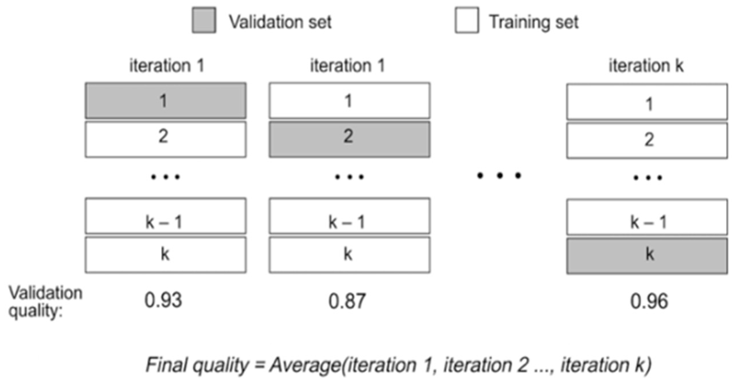
2.2. Cross Validation

Cross validation (CV) [21] is a model estimation technique which was used in our research for fitness evaluation. As we mentioned earlier in Section 1, the proposed emergency braking support system would be based on a classifier of the emergency braking situations. For calculating the CV score (fitness value), the available dataset is divided into k subsets, or folds. The classifier is trained on k−1 folds and its performance is validated on the remaining k fold. The process performed k iterations using every fold for validation. The CV score of the classifier was calculated by averaging the validation quality of each iteration. Despite the computational overhead of calculating the CV score, it was rather parsimonious in terms of the required amount of data. Also, it was shown to prevent overfitting of the obtained solutions [21]. The k-fold CV is illustrated in Figure 4.

As a score of CV, different quality metrics could be used, as elaborated below.

2.3. Quality Metrics

For the binary classification problems, the following metrics are usually considered [22]: accuracy, precision, recall, f-score, and area under the receiver operating characteristic curve (ROC AUC). All these metrics reflects different aspects of the classifier. However, for the comparability of our experimental results with the results of previous studies, we would leave ROC AUC out of consideration. Regarding accuracy, this metric reflects the percentage of the correct answers. For the determination of the other metrics, we shall consider the confusion matrix as shown in

Table 1. Confusion matrix.

		Actual Condition
		Positive	Negative
Predicted Condition	Positive	True positive (TP)	False positive (FP)
	Negative	True negative (TN)	False negative (FN)

.

From herein, we will refer to the cases of emergency braking as class “1”, and normal driving cases as class “0”. TP reflects the number of time series samples of class “1” (human-annotated), that are correctly classified. FP corresponds to the samples for which the correct, human-annotated class is “0”, but the classifier returns “1”. Conversely, if the classifier returns “0” but the actual class is “1”, then the sample is considered as FN. Finally, TN reflects the number of samples of class “0” that are correctly classified. Hence, the precision and recall are defined as follows:

$$Precision=\frac{TP}{\left(TP+FP\right)}$$

(1)

$$Recall=\frac{TP}{\left(TP+FN\right)}$$

(2)

From the Equations (1) and (2) we can express f-score, which is a harmonic mean of both precision and recall:

$$F=2\times \frac{Precision\times Recall}{Precision+Recall}$$

(3)

As can be seen from Equation (3), the f-score reaches its maximum value of 1.0 when the values of both precision and recall are 1.0 (maximum value).

2.4. Extreme Gradient Boosting

Extreme gradient boosting or XGBoost [23] is a scalable machine learning algorithm that is widely used in many supervised machine learning challenges [24,25]. XGBoost produces the classification or regression model as an ensemble of K classification and regression trees (CART) [26]. The output of the model can be expressed as follows:

$$\widehat{y}=\phi \left(X_i\right)={\displaystyle \sum }_{k=1}^K{f}_k\left(X_i\right), f_k\in F$$

(4)

where $f_k$ corresponds to independent tree structure and leaf weights, while $X_i$ is a test sample which can be expressed as a vector of features $\left(x_{i0},x_{i1},\dots ,x_{in}\right)$. $F$ represents a test space of all CART. For training the set of functions used in the model, the following regularized objective must be minimized:

$$L\left(\phi \right)={\displaystyle \sum }_{i}l(\widehat{y_i},y_i)+{\displaystyle \sum }_k\mathsf{\Omega }\left(f_k\right)$$

(5)

The first term l of Equation (5) is differentiable convex loss function which calculates the difference between target $y_i$ and predicted $\widehat{y_i}$. The second term Ω is a regularization that prevents over-fitting by penalizing the complexity of the model.

The XGBoost classifier is also known for its superior training speed. The latter is crucial for the running time of the coevolution, since the training of XGBoost is executed during each evaluation of the fitness.

2.5. Wilcoxon Signed Rank Test

In our work, we examined the significant differences between the results obtained within CC and GA [13]. Hence we employed a non-parametric statistical hypothesis test, namely the Wilcoxon signed-rank test [27] which ranks the differences in performances of two algorithms. This test ignores the signs and compares the ranks for the positive and negative differences.

Let $d_i$ be the difference between the performance scores of the two algorithms on the $i$-th run out of n. The differences are ranked according to their absolute values; average ranks are assigned in the case of ties. Let $R^{+}$ be the sum of ranks where the second algorithm performed better than the first one, and $R^{-}$ the sum of ranks for the opposite case. If $d_i=0$, the ranks are split evenly among the sums; if there is an odd number of them, one is ignored. The critical values of $T=\min \left(R^{+},R^{-}\right)$ for number of runs up to 25 can be found in the book on general statistics [28]. For a larger number, z-score must be calculated.

$$z=\frac{T-\frac{1}{4}N\left(N+1\right)}{\sqrt{\frac{1}{24}N\left(N+1\right)\left(2N+1\right)}}$$

(6)

For the significance level $\alpha =0.05$ the null-hypothesis (both models perform equally) can be rejected if the z-score is smaller than $-1.96$.

3. Proposed Approach

In order to achieve our objective of discovering the optimal combination of features and the values of hyperparameters that would potentially improve the performance of the classifier for EBC problem, we organized our research into the following four consecutive stages: (i) obtaining and analyzing the time series of the movement of the accelerator- and brake pedals of a car simulated in a full-scale drive simulator, (ii) adopting CC for evolving features from the acquired time series and the values of the hyperparameters of XGBoost, (iii) evaluating the performance of XGBoost with the evolved solution on unforeseen data; and, finally, (iv) comparing the final solution for EBC problem with the results of previously published research. We will elaborate on these stages in the following Section 4 and Section 5.

4. Methodology

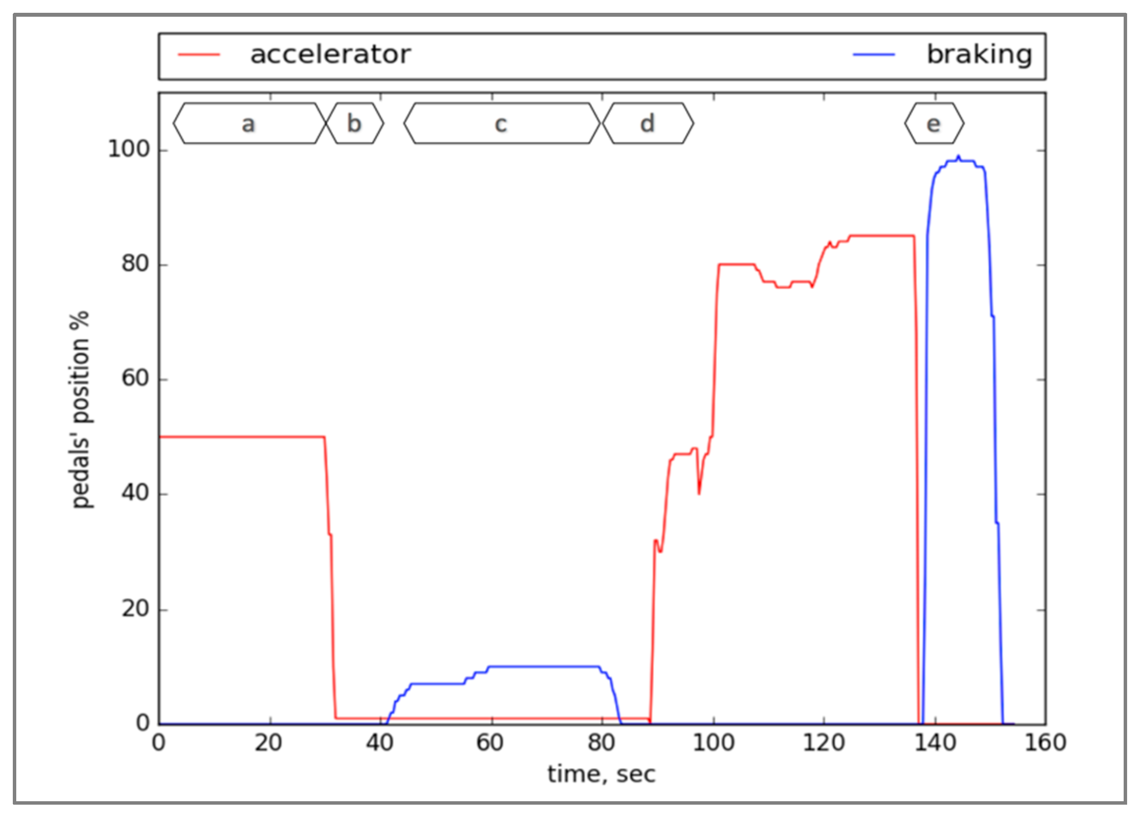
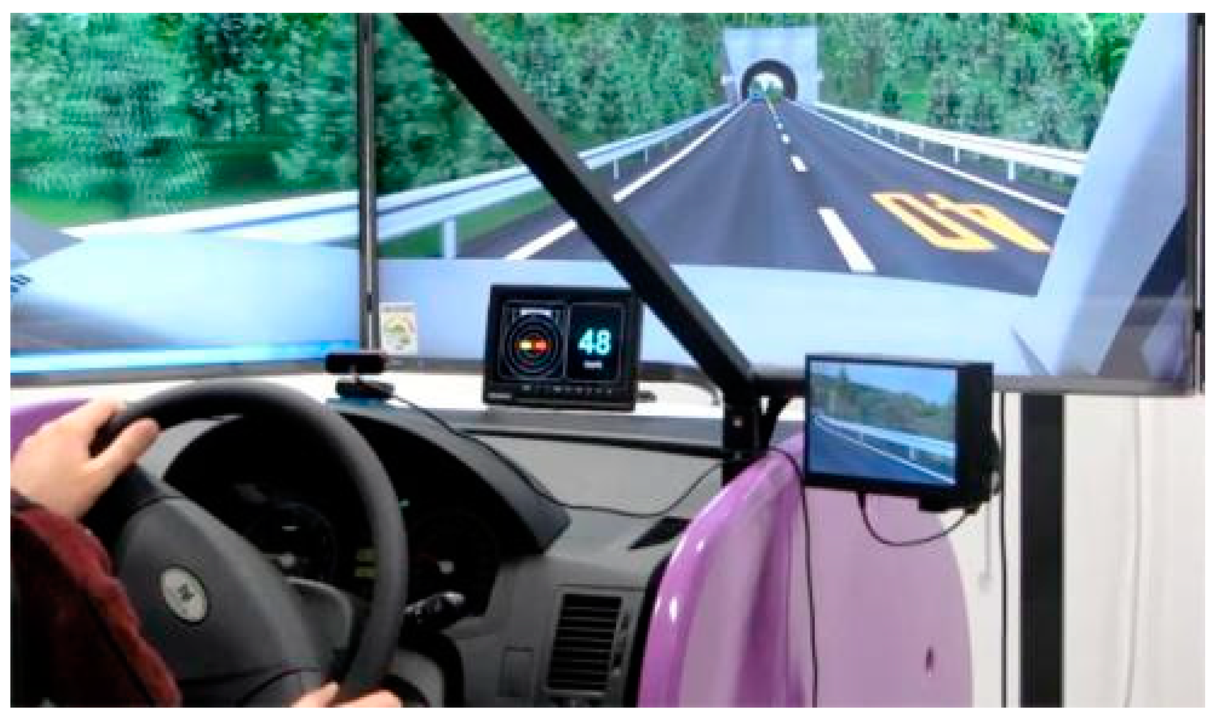
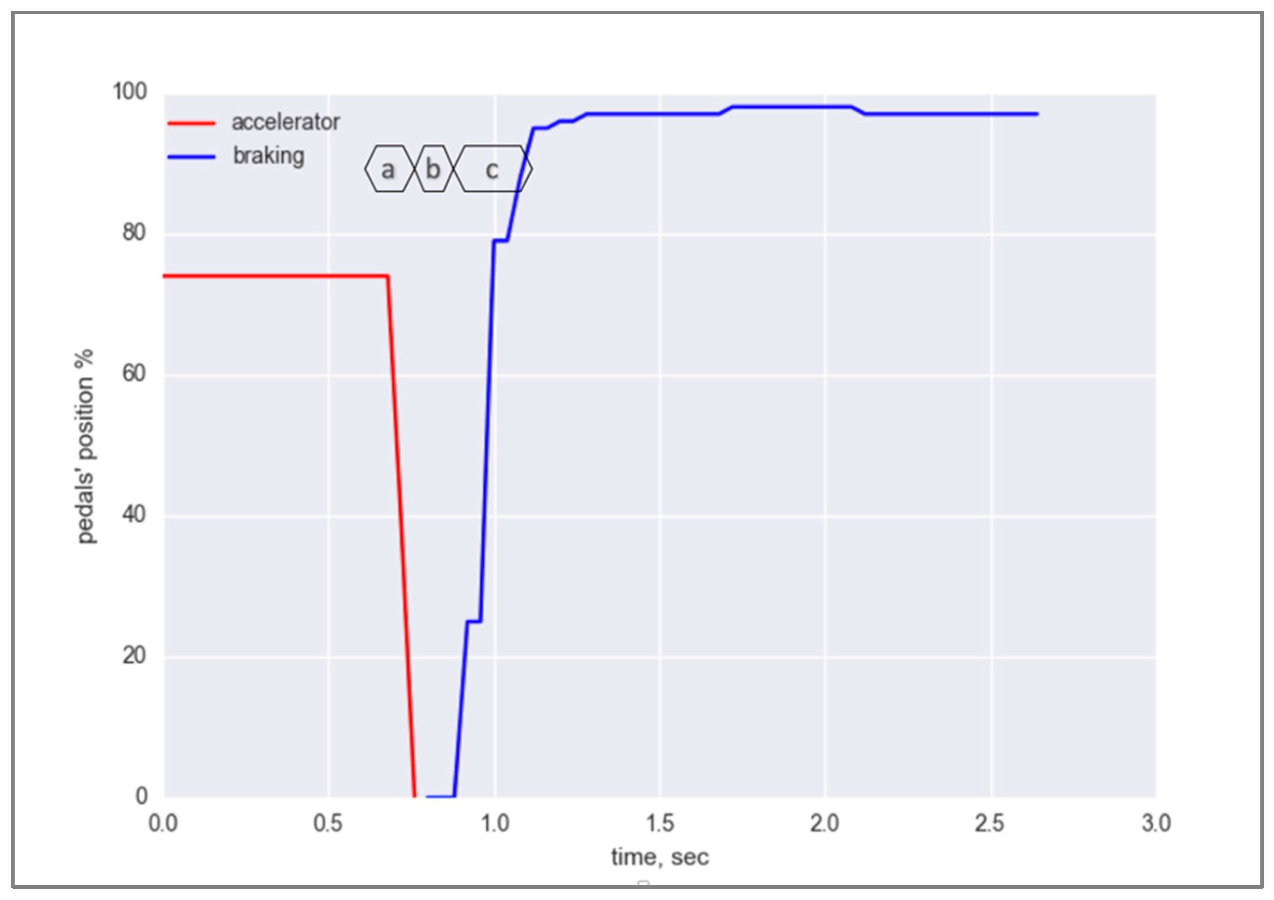
4.1. Data Collection and Analysis

For obtaining the time series that represent the motion of the pedals, we asked 16 human drivers (men and women, aged 20–52) to drive a simulated car featuring an automatic transmission [12] in various tracks. The details of the tracks are shown in

Table 2. Details of experimental tracks.

Track	Road Conditions	Traffic Conditions
Highway	Dry, wet	Moderate, high-speed traffic
City road	Dry	Empty road (no traffic)
Country side	Both dry and wet	Dense, low-speed traffic

. All the testers were required to have a driver license and to practice the driving of the car on the simulator. After practicing, all testers participated in two separate experiments which allowed us to split the data carefully into two classes: normal driving and emergency braking, respectively. The details of experiments are elaborated in

Table 3. Details of the two series of experiments.

Experiment	Requirements	Number of Samples
Normal driving	Emergency braking is not allowed	1659
Emergency braking	Audible signal prompts the drivers to apply emergency braking	714

.

For experiments with normal driving, the drivers had to drive a car without applying emergency braking. In contrast, during the experiments with emergency braking, they were asked to apply the emergency brake at the time that they hear a special audible signal. This way of signalling imitates the sudden danger on the road. We assumed that there is no difference between the responses of drivers to a real danger and to the audible signal. When the drivers heard the signal, they were requested to release the accelerator and press the brake pedal to its maximum position as soon as possible.

Despite the fact that the drivers were asked not to use normal brakes during emergency braking experiments and not to use emergency brakes during normal driving experiments, due to various human factors, we could not be completely sure that this would be the case. For instance, during normal driving experiments, the driver could accidentally apply emergency brakes if they considered the actual traffic situation to be dangerous. Therefore, it was necessary for us to annotate the obtained time series data of the accelerator pedal carefully. However, due to the impossibility of the human annotator to handle all these “mistakes”, the final dataset could still contain some mislabeled samples.

The simulated parametric data recorder captured all of the relevant time series of the position of both pedals (within the range 0%…100%), sampled with a frequency of 25 Hz. During the processing of the mentioned time series, we extracted 2373 events in total, including both normal driving (class “0”) and emergency braking (class “1”) events. Sample fragments of the obtained time series of position of accelerator pedal are shown in

Table 4. Sample fragments of the time series of the position of accelerator pedal (in percent).

Fragment of the Time Series	Corresponding Class
{0, 20, 22, 20, 15, 9, 3, 2, 1}	“0” (Normal driving)
{0, 10, 20, 19, 23, 2, 1}	“1” (Emergency braking)
{0, 50, 74, 72, 67, 58, 45, 24, 4, 1}	“0” (Normal driving)
{0, 13, 30, 40, 30, 45, 72, 68, 68, 65, 61, 22, 1}	“1” (Emergency braking)

. As Table 4 illustrates, each fragment consists of a series of changing positions of the accelerator pedal, where the first member of the series corresponds to the moment when the accelerator was pressed, while the last one to the moment when the accelerator pedal returned to its initial position.

The proposed approach of collecting the data is a fundamental difference between our previous and current research. In our previous studies, we only considered the decreasing sequence of the position of the accelerator pedal, leaving the remaining part of series out of our scope. As will be seen in the next paragraphs, the new approach offered much more flexibility for the analysis of drivers’ behaviour. As the series were defined by the dynamics of their values, rather than the number of entities, the first in, first out (FIFO)-buffer that should eventually store these fragments should be of a variable size too. This might add to the complexity of the considered classification problem, as the input of the classifier in general, should be of a fixed size.

4.2. Implementation of the Cooperative Coevolution

As we briefly mentioned in Section 2, we represent the individuals as a conjunction of forest and chromosome as depicted in Figure 5.

4.2.1. Set of Terminals in the Trees of the Forest

Firstly, it is necessary to determine the set of terminal symbols in trees that represent the arithmetic expressions of features pertinent to the dynamics of the accelerator pedal. Because the initial task deals with the classification of samples which have variable size, we decided to propose as terminals a set of primitive (atomic) functions that are invariant to the length of the time series of the positions of the accelerator pedal. Unlike the a priori predefined permutations of the extracted features in [13], the proposed functions took into account a longer history of the dynamics of the accelerator—the movements of the pedal preceding the final deceleration. The atomic functions that comprise the terminal set of the trees in the forest evolution are shown in

Table 5. Atomic functions that are invariant to the length of the time series.

Function	Meaning	Example
mean (buf)	mean of the last decreasing subsequent	mean ({0, 10, 50, 2, 0}) = 17.3
std (buf)	standard deviation of the last decreasing subsequence	std ({0, 10, 50, 2, 0}) = 23.1
max (buf, i)	i-th maximum element of the buffer	max ({0, 10, 50, 2, 0}, 0) = 50 max ({0, 10, 50, 2, 0}, 1) = 2
mdelta (buf, i)	i-th maximum delta of the buffer	mdelta ({0, 10, 50, 2, 0}, 0) = 48 mdelta ({0, 10, 50, 2, 0}, 0) = 2
suminc (buf) sumdec (buf)	average sum of all increasing/decreasing subsequences	suminc ({0, 10, 50, 2, 0}) = 20 sumdec ({0, 10, 50, 2, 0}) = 17.3
auf (buf)	area under the buffer, dx = 1	suminc ({0, 10, 50, 2, 0}) = 20
aud (buf)	area under the last decreasing subsequence, dx = 1	aud ({0, 10, 50, 2, 0}) = 27
maxinc (buf) mininc (buf)	maximum/minimum between all averages of increasing subsequences	maxinc ({0, 10, 50, 2, 0}) = 20 mininc ({0, 10, 50, 2, 0}) = 20
maxdec (buf) mindec (buf)	maximum/minimum between all averages of decreasing subsequences	maxdec ({0, 10, 50, 2, 0}) = 17.3 mindec ({0, 10, 50, 2, 0}) = 17.3
fullmean (buf)	average value of the buffer	fullmean ({0, 10, 50, 2, 0}) = 12.4
fullstd (buf)	standard deviation value of the buffer	fullstd ({0, 10, 50, 2, 0}) = 19.6
dlen (buf)	length of last decreasing subsequent	dlen ({0, 10, 50, 2, 0}) = 3

.

Thus, the domain of the defined atomic functions is a set of the values of positions of accelerator pedal $\left(p_n,p_{n-1},\dots ,p_0\right)$ where $n\in N$. However, for the functions $\max \left(buf,i\right)$ and $\mathrm{mdelta}\left(buf,i\right),$ there may be exceptions that arise when $i>n$. Therefore, we programmed these functions in the way that is tolerant to such exceptions. If $i>n$ the function will be recursively recalled until $i\le n$. For instance, $\max \left(\left\{0,25,50,2,0\right\},3\right)$ will return 0 as well as $\max \left(\left\{0,25,50,2,0\right\},2\right)$. Besides the defined functions, we added a random constant $c\in \mathbb{N}$: to our terminal set TS, hence the latter became: $TS=\left\{\mathrm{mean}\left(buf\right),\mathrm{std}\left(buf\right),\mathrm{mdelta}\left(buf,i\right),\max \left(buf,i\right),c,\right\}$.

4.2.2. Set of Function in the Trees of the Forest

The set of functions in GP included four binary (i.e., requiring two arguments) arithmetical functions {+, −, ×, /}—addition, subtraction, multiplication, and (protected) division.

4.2.3. Evolving the Features

In a bid to evolve the features, we use a forest of several parse trees representing the evolved individual. The forest could contain up to eight trees. The number of trees in the forest was not fixed and might vary as a result of implementing the crossover and mutation operations in due course of the evolution. Each tree in the forest encoded an evolved (compound) feature, and it contained functional- and terminal nodes from the above-mentioned set of functions and terminals of the trees, respectively. An example of an individual, represented as a forest of two trees (features), is shown Figure 6. After parsing this example tree in a depth-first left-to-right manner, we would obtain the following set of two features: $\left\{\frac{\max \left(buf,0\right)}{\mathrm{mean}\left(buf\right)},\mathrm{std}\left(buf\right)\right\}$.

4.2.4. Evolving the Hyperparameters

As it was mentioned above, for evolving the hyperparameters, we utilized the chromosomes that contain the discretized values of XGBoost hyperparameters. The ranges and discretized values of the hyperparameters of XGBoost are shown in

Table 6. Content of chromosome for optimizing the values of hyperparameters of XGBoost.

Hyperparameter	Interval of Discretization	Range	Meaning
eta	0.002	[0, 1]	Step size shrinkage. Controls the learning rate in update and prevents overfitting
gamma	0.1	[0, 100]	Minimum loss reduction required to make a node split. The split happens when the resulting split gives a positive reduction in the loss function.
max depth	1	[1, 20]	The maximum depth of a tree
min child weight	1	[1, 100]	Minimum sum of weights of all observations required in a child
subsample	0.002	[0.001, 1]	Subsample ratio of the training instance
colsample by tree	0.001	[0.5, 1]	Subsample ratio of columns when constructing each tree
n estimators	1	[100, 500]	The number of boosting stages to perform

.

4.2.5. Fitness Function

The objective of applying GP is to search for optimal set of features that results in the best value of the fitness function (i.e., CV score). In order to determine the metric which must be used for calculating the CV score, it is important to analyze the class distribution of the available data.

The training set which was used during the cross validation included 536 samples of class “1” and 1069 of class “0”. If we used accuracy as a fitness function it could lead to incorrect quality assessment: if the learned XGBoost detected all normal driving samples and missed more than a half of emergency braking samples, the cross validation score could still reach the value of 0.83; however our classifier would not be considered as reliable. Therefore, instead of using the raw CV accuracy as a fitness function, we used a more informative metric—the f-score, which is the harmonic mean of precision and recall. There are two major reasons why we were reluctant to use precision or recall as a fitness function:

• These metrics describe different aspects of the classifier. It is not evident which metric is more preferable for building the emergency braking system, and
• The consideration of only precision or recall as fitness function can lead to the phenomenon known as “evolutionary cheating”. For instance, evolution will choose the features that decrease the number of FP, without any respect to FN. Consequently, the precision might even become 1.0, however the recall will be significantly lower.

Conversely, the f-score is a good tradeoff between the values of precision and recall. For the sake of avoiding the meaningless features in our final solution, we added a penalty that subtracts 1% of fitness values if the resulting features are nothing but constants.

4.2.6. Main Parameters of Coevolution

The considered size of the evolved population of individuals (forest and chromosome) is 200, as indicated by the parameter Population size in

Table 7. Main parameters of the coevolution.

Parameter	Value
Genotype	Conjunction of forest and chromosome
Population size	200 individuals
Selection	Binary tournament
Selection ratio	10%
Elite	Best 4 individuals
Crossover	Single-point
Mutation	Single-point
Mutation ratio	5%
Fitness value	Cross validation (CV) f-score, with 1% subtraction penalty
Termination criteria	(# Generations > 200) or (Fitness value = 100%)

. The mating pool of each following generation consists of 24 individuals. Part (20 individuals, or 10% of population) of the mating pool is selected via a binary tournament selection (parameter Selection ratio) plus the best (elite) four individuals (parameter Elite in Table 7). The number of elite individuals is selected empirically to provide the best trade-off between the convergence of evolution (yet preventing the premature convergence to suboptimal solutions) and diversity of population. The remaining 176 (of 200) individuals are produced by single-point crossover operations (parameter Crossover in Table 6) on pairs of forests, randomly selected from the individuals in the mating pool. The newly produced trees are mutated via single-point mutation (parameter Mutation in Table 7) with a probability of 5% (parameter Mutation ratio in Table 7). The details of the implementation of the binary selection, single-point crossover, and mutation operations are provided in [29].

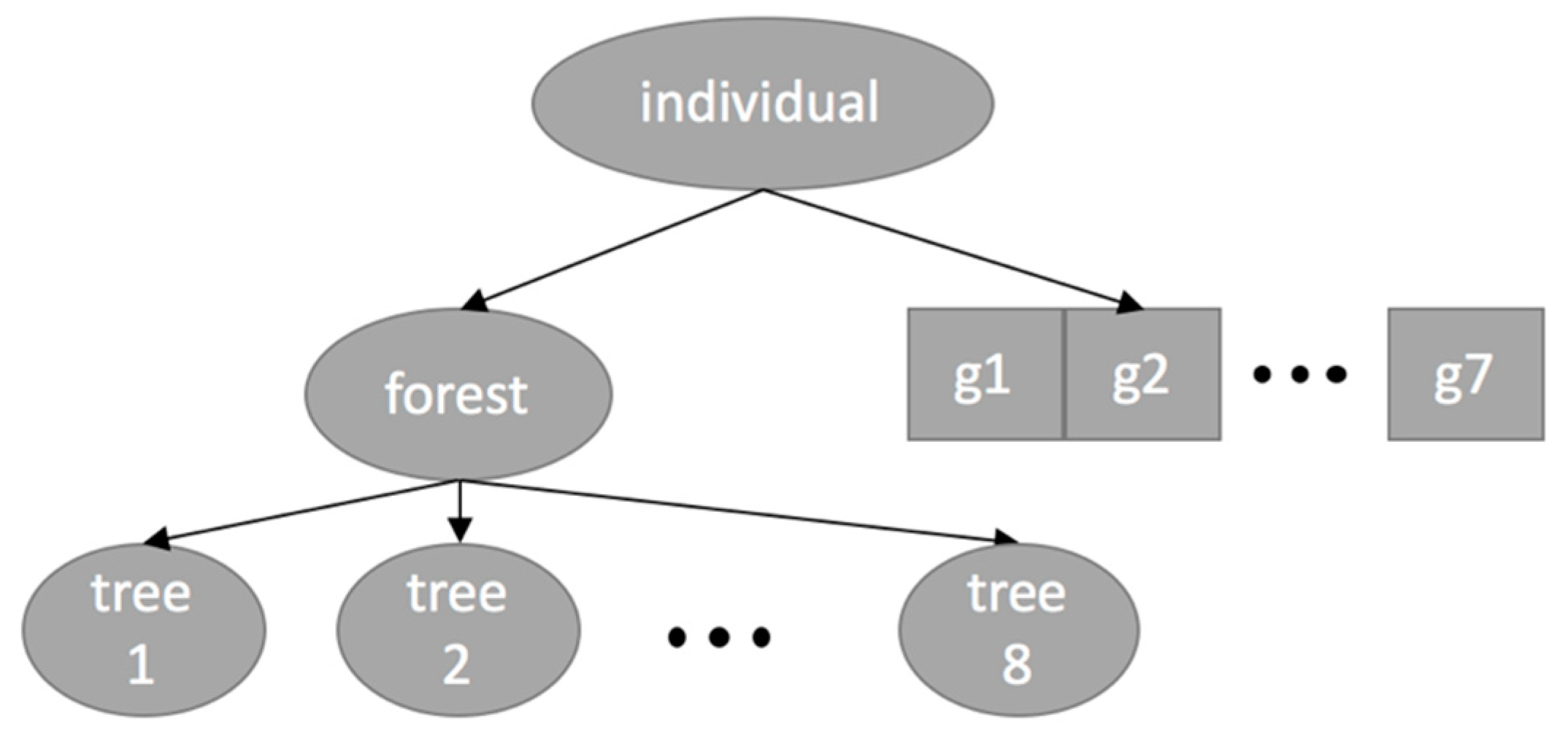
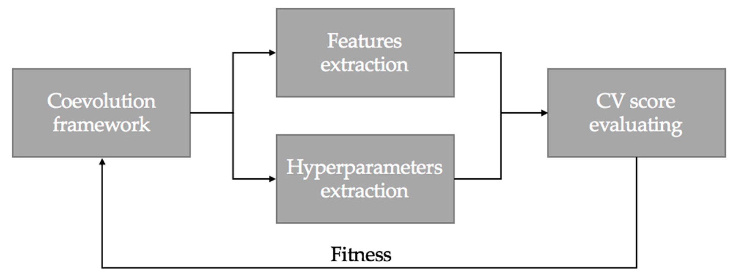
4.2.7. The Entire System

The mechanism of coevolving the features pertinent to the dynamics of accelerator pedal and the values of the hyperparameters of the classifier is illustrated in Figure 7. The mechanism consisted of the following eight main steps:

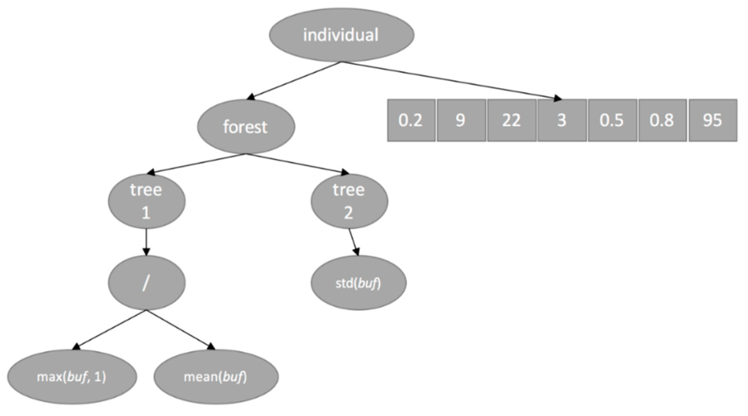
• Initialization: Generating the random initial population of 200 individuals. Each individual is a conjunction of forest and chromosome. The forest can contain up to eight trees (features), while the number of genes (hyperparameters) is fixed and equal to 7.
• Fitness evaluation, phase A: Obtaining the sets of features and hyperparameters for each individual by parsing the trees in the forest and the linear chromosome.
• Fitness evaluation, phase B: Extracting the values of each of the features from the raw time series of accelerator pedal.
• Fitness evaluation, phase C: Calculating the fitness value of each individual (set of features) as a CV f-score of XGBoost classifier that uses the obtained hyperparameters and calculated features.
• Checking the termination criteria. Terminating if any of them has been satisfied.
• Selection: based on the obtained fitness values of all individuals, selecting the mating pool of 24 individuals via binary tournament and elitism.
• Reproduction: Reproducing the population via crossover of individuals in the mating pool and mutation of offspring.
• Continuing with step 2.

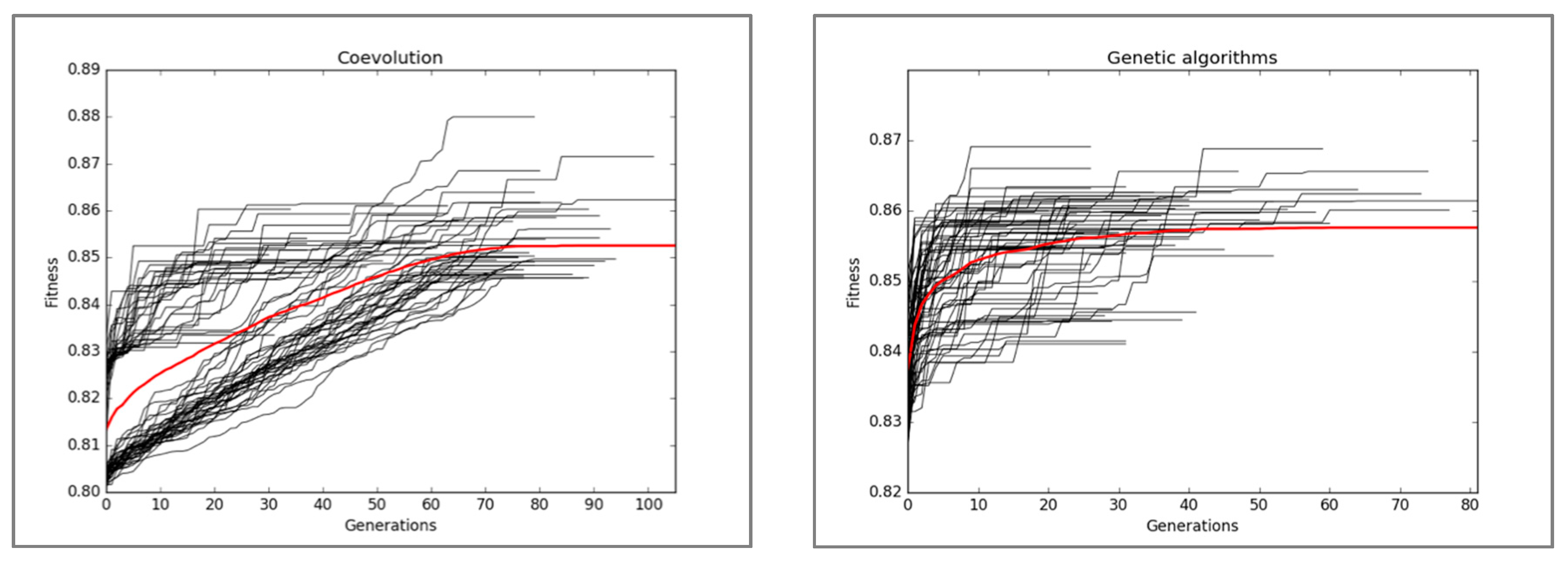
5. Experimental Results

The implementation of XGBoost classifier is based on an open source package of XGBoost [30] that supports multiple programming languages including C++, Python, R, Java, Scala, and Julia.

To comparatively evaluate the quality of EBCs based on evolved (via CC) features and hyperparameters, as a benchmark we also used XGBoost classifiers with evolved (via GA) optimal values of its hyperparameters [13]. For each evolutionary algorithm we performed 50 independent runs and consequently obtained 100 classifiers (50 within GA, 50 within CC). For GA, we preserved the parameters that were used in the corresponding studies as shown in

Table 8. Main parameters of the GA for the evolution of values of hyperparameters of the classifier.

Parameter	Value
Genotype	Set of parameters shown in Table 6 and fixed combination of features (pertinent to the last decreasing subsequence of the buffer). Among them are the highest position of the accelerator pedal before starting the deceleration (mP), the maximum and average rate of lifting the accelerator (mR and aR respectively)
Population size	40 individuals
Selection	Binary tournament
Selection ratio	10%
Elite	Best two individuals
Crossover	Single-point
Mutation	Single-point
Mutation ratio	5%
Fitness value	CV f-score
Termination criteria	(# Generations > 100) or (Fitness value = 100%)

.

The convergence of the fitness value (CV f-score) during 50 independent runs of CC and GA for XGBoost classifiers is shown in Figure 8.

5.1. Statistical Significance Test

In order to show the statistical significance of the results, each classifier was tested on unforeseen data (test set) with respect to f-score. The full comparative table of 100 classifiers can be accessed online from the web site of the first author [30]. As it turned out, 31 EBCs that were obtained within CC performed better than classifiers obtained within GA, and 19 showed slightly worse results. Upon implementing the Wilcoxon signed rank test with significance level $\alpha =0.05$, we obtained $z-\mathrm{score}=–2.12854794772$ which suggests to us that the resulting difference was significant.

5.2. Best Solutions Comparison

In this subsection, we compared the best solutions (highest fitness value) that were obtained by coevolution (xgb_cc) and genetic algorithm (xgb_ga). The performance of classifiers on both training and test sets is shown in

Table 9. Performance of best classifiers on training and test set.

Metric	xgbga		xgbcc
	Training Set	Test Set	Training Set	Test Set
Accuracy	0.9052959	0.9036458	0.9850467	0.9466146
Precision	0.8609022	0.7988506	0.9776119	0.9254658
Recall	0.8544776	0.7808989	0.9776119	0.8370789
f-score	0.8576779	0.7897727	0.9776119	0.8790560

.

As can be seen in Table 9, xgb_cc outperformed xgb_ga with respect to each considered metric for training and test sets. More detailed performance on test set is provided in

Table 10. Performance of best classifiers on training and test set.

Classifier	TP	TN	FP	FN
xgbga	139	555	35	39
xgbcc	149	578	12	29

.

The evolved features and their relative importance are shown in

Table 11. Evolved features.

#	xgbga Features	xgbga Features Importance	xgbcc Features	xgbcc Features Importance
1	mP	0.17105263	$\mathrm{dlen}\left(buf\right)$	0.14775977
2	mR	0.30263159	$\mathrm{mdelta}\left(buf,0\right)$	0.15157293
3	aR	0.30263159	$\mathrm{fullstd}\left(buf\right)$	0.16301239
4	mP$\times$aR	0.22368421	$\mathrm{fullmean}\left(buf\right)$	0.1749285
5	­	­	$3\times \mathrm{mdelta}\left(buf,2\right)$	0.08674929
6	­	­	$\frac{\mathrm{mdelta}\left(buf,1\right)}{\mathrm{std}\left(buf\right)-\mathrm{dlen}\left(buf\right)}$	0.0729266
7	­	­	$$\begin{gathered} \left(\mathrm{std}\left(buf\right)+8\right)\times (\max \left(buf,2\right) \\ +\left(\mathrm{mean}\left(buf\right)\times \mathrm{aub}\left(buf\right)-8\right)) \end{gathered}$$	0.20305052

. The importance measures are based on the number of times a feature is selected for splitting, weighted by the squared improvement to the model as a result of each split, and averaged over all trees.

It is important to note again that features that were obtained within GA took into account only the last decreasing subsequence of the accelerator pedal positions, which limited the scope of evolutionary creativity and flexibility. Thus, features #3, #4, and #7 obtained within CC leveraged the whole buffer. Moreover, feature #7 had the highest importance value in comparison with the other features that are used by xgb_cc. Evolution of features was closely linked to the evolution of hyperparameters. The values of hyperparameters that yielded the best EBCs are shown in

Table 12. Evolved hyperparameters.

Hyperparameter	xgbga	xgbcc
eta	0.1840816	0.080092
gamma	8.1	1.6
max depth	18	14
min child weight	2	1
subsample	0.4660533 (9)	0.70003
colsample by tree	0.7 (3)	0.71 (8)
n estimators	145	144

.

We noticed that similar to the results obtained via other nature-inspired optimization approaches (e.g., memetic algorithms, genetic programming, neural networks, etc.), the solutions evolved via CC and GA were hard to interpret due to (i) the complexity of the computational structures the hyperparameters defined, (ii) the complexity of the mathematical representations of several features, and (ii) the lack of any human-understandable logic—similar to that of the “canonical” top-down problem-solving approaches—expressed in these features.

6. Discussion

The coevolution of the features and the classifier implies that the overall computational overhead of the real-world implementation of the brake assisting system would consist of two components corresponding to the following two classification stages: (i) calculating the values of the features in accordance with the evolved (via GP) algebraic expression, and (ii) classifying the braking situations from the calculated features by the (tuned by GA) XGBoost classifier. These two classification stages are activated in real time as soon as the position of the accelerator pedal becomes 0. We measured the computational overhead of these two classification stages on a PC with x64-based Intel Core i7-6700 3.4 GHz CPU and 16 GB of RAM. The mean and maximum values of the overhead are shown in

Table 13. Computational overhead of the brake-assisting system.

Stage	Mean Overhead, ms	Maximum Overhead, ms
Stage 1: Feature calculation	0.323	2.005
Stage 2: Classification	0.252	0.515
Overall	0.575	2.520

. We estimated the maximum overall overhead with the assumption of a hypothetic worst-case scenario when the computational overhead of both stages is at its maximum.

As shown in Table 13, on average, the computational overhead is about 0.6 ms, which is less than 0.3% of the average time lag between the instant when the drivers lift the accelerator and then press the brake pedal (about 200 ms). At worst, the brake assisting system would be activated with a delay of about 2.5 ms, which is still negligible compared to the delays of the driver’s reaction.

False Positives

In real-driving situations, the FP errors committed by the classifier can cause an incorrect applying of emergency braking. As the research of Podusenko et al. [13] suggests, generally, for the emergency braking systems under consideration, the false positives will not necessarily lead to an accident, as the emergency braking could be applied just for a very brief period of time that is equivalent to the average delay of the drivers’ response.

Nevertheless, both false positives and false negatives are undesirable in EBS. The errors of the considered classifier occurred on the test set could be attributed to the following factors:

• Mislabelled (by a human expert) samples in the whole dataset,
• Lack of a sufficient number of samples featuring a similar trend,
• Personal traits of the drivers that result in contradictory data for the classifier, and
• XGBoost could not capture the underlying trends of the data.

While the fourth reason is very unlikely [25,26], the others are likely to occur.

Contradicting samples are samples that have exactly the same features but belong to different classes. This unfortunate phenomenon can be easily demonstrated by the following example. Considering two-real samples from two different drivers:

• sample1 = {0, 7, 7, 7, 21, 35, 37, 37, 38, 38, 39, 41, 43, 45, 46, 47, 48, 48, 49, 49, 50, 50, 52, 53, 54, 54, 54, 54, 54, 54, 54, 54, 54, 54, 54, 54, 55, 55, 55, 55, 55, 55, 55, 55, 55, 55, 55, 55, 55, 55, 55, 55, 55, 55, 55, 55, 55, 55, 55, 55, 55, 55, 55, 55, 55, 55, 55, 55, 55, 55, 55, 55, 55, 55, 55, 55, 55, 55, 55, 55, 55, 55, 55, 55, 55, 55, 55, 55, 55, 54, 54, 54, 54, 53, 54, 54, 53, 53, 53, 53, 53, 53, 53, 53, 53, 53, 52, 53, 53, 53, 53, 53, 53, 53, 53, 53, 53, 53, 53, 53, 53, 53, 53, 20, 20, 1}
• sample2 = {0, 17, 17, 31, 31, 34, 34, 35, 36, 36, 37, 39, 40, 41, 41, 41, 42, 42, 42, 42, 42, 42, 42, 42, 42, 42, 42, 42, 42, 42, 42, 42, 42, 42, 42, 42, 40, 40, 40, 40, 40, 40, 40, 40, 40, 40, 41, 42, 44, 44, 45, 45, 45, 45, 45, 46, 46, 47, 47, 48, 48, 49, 49, 49, 49, 49, 49, 50, 50, 50, 50, 50, 50, 50, 50, 50, 50, 50, 50, 50, 50, 50, 50, 50, 50, 50, 50, 50, 50, 50, 50, 50, 50, 50, 50, 50, 50, 50, 50, 50, 50, 50, 50, 50, 50, 50, 50, 50, 50, 50, 50, 50, 50, 50, 50, 50, 50, 50, 50, 50, 50, 50, 50, 50, 50, 50, 50, 50, 50, 50, 50, 51, 51, 51, 51, 51, 51, 51, 52, 52, 52, 52, 53, 53, 53, 53, 35, 2, 1}

Obviously, the buffers have several different properties; however as can be seen from

Table 14. Example of samples’ classification.

Classifier	Sample	Extracted	Output	Real Class
xgbga	1	[53, 825, 433.3, 22,966.6]	1	1
	2	[53, 825, 433.3, 22,966.6]	1	0
xgbcc	1	[5,981,896.76, 49.98, 11.31, 33, 3, 1, 38]	1	1
	2	[4,625,878.23, 45.21, 8.76, 33, 3, 0.99, 4]	0	0

, the features that are extracted by means of GA are identical. Conversely, coevolution allowed us to distinguish these samples and consequently to classify them properly.

From the perspective of xgb_ga, the number of contradicting pairs is 16:12 in training and four in test sets. This disadvantage is almost absent in the classifier that has been evolved within coevolution (only one conflict pair in training set).

Despite the fact that CC addresses the problem of conflicting duplicates, the presence of contradicting samples is not fully resolved. Through the analysis of erroneously classified samples, we noticed, that there are several similar pairs obtained from different drivers yet annotated differently. These samples remain extremely difficult for each evolved classifier. Therefore, learning the classifier to classify the driving style of a particular driver, rather than attempting to classify the actually non-existent “average” driver, might result in further increase of the reliability of classification. Hence, in our future research, we are planning to categorize the drivers according to the way they operate the pedals.

7. Conclusions

We examined the feasibility of improving the XGBoost classifier for the EBC problem by applying cooperative coevolution for evolving the optimal set of features of the time series of accelerator pedal and hyperparameters of the classifier. We showed that the resulting difference between the classifiers that were trained by means of coevolution and genetic algorithms is statistically significant. We also compared the quality of best classifiers and demonstrated the superiority of xgb_cc over xgb_ga. The experimental results suggest that the evolving both features and hyperparameters via CC could, indeed, result in a classifier that detects the EBS with an accuracy of about 95% on an unforeseen test set of time series data for the dynamics of the accelerator pedal.

Moreover, the features that are obtained by CC are particularly beneficial since they allow to avoid the conflicting duplicates that increase the performance of the classifier’s decision-making mechanism.

We also considered the possibility of utilizing the proposed braking agent in real motor vehicles. Taking into account the execution speed of the feature extraction and classification, this type of braking assistance makes it possible to substantially reduce the time lag without any significant loss.

In our future work, we are planning to investigate the ways to further improve the quality of the classifier. We are especially interested in exploring the possibility of adapting the learned, yet generic classifier to the driving style of a particular driver by real-time (online) learning.

References

1. 13 Advanced Driver Assistance Systems. Available online: https://www.lifewire.com/advanced-driver-assistance-systems-534859 (accessed on 20 June 2018).
2. Wikipedia. List of Countries by Traffic-Related Death Rate. 2018. Available online: https://en.wikipedia.org/wiki/List_of_countries_by_traffic-related_death_rate (accessed on 20 June 2018).
3. Coelingh, E.; Eidehall, A.; Bengtsson, M. Collision Warning with Full Auto Brake and Pedestrian Detection—A practical example of Automatic Emergency Braking. In Proceedings of the 13th International IEEE Conference on Intelligent Transportation Systems, Funchal, Portugal, 19–22 September 2010; pp. 155–160. [Google Scholar]
4. Coelingh, E.; Jakobsson, L.; Lind, H.; Lindman, M. Collision Warning with Auto Brake—A Real-Life Safety Perspective. In Proceedings of the 20th International Technical Conference on the Enhanced Safety of Vehicles (ESV), Lyon, France, 18–21 July 2007. [Google Scholar]
5. Kusano, K.D.; Gabler, H.C. Safety Benefits of Forward Collision Warning, Brake Assist, and Autonomous Braking Systems in Rear-End Collisions. IEEE Trans. Intell. Transp. Syst. 2012, 13, 1546–1555. [Google Scholar] [CrossRef]
6. Fancher, P.; Bareket, Z.; Ervin, R. Human-Centered Design of an Acc—With Braking and Forward-Crash-Warning System. Int. J. Veh. Mech. Mobil. 2001, 36, 203–223. [Google Scholar] [CrossRef]
7. Wilde, G.J.S. The theory of risk homeostasis: Implications for safety and health. Risk Anal. 1982, 2, 209–225. [Google Scholar] [CrossRef]
8. Podusenko, A.; Nikulin, V.; Tanev, I.; Shimohara, K. Cause and Effect Relationship between the Dynamics of Accelerator and Brake Pedals during Emergency Braking. In Proceedings of the FAST-Zero’17, Nara, Japan, 18–22 September 2017. [Google Scholar]
9. Kiesewetter, W.; Klinkner, W.; Reichelt, W.; Steiner, M. Der neue Brake-Assist von Mercedes-Benz. Automobiltechnische Zeitschrift 1997, 6, 330–339. [Google Scholar]
10. Haufe, S.; Kim, J.; Kim, I.H.; Treder, M.S.; Sonnleitner, A.; Schrauf, M.; Curio, G.; Blankertz, B. Electrophysiology-based detection of emergency braking intention in real-world driving. J. Neural Eng. 2014, 11, 056011. [Google Scholar] [CrossRef] [PubMed]
11. Podusenko, A.; Nikulin, V.; Tanev, I.; Shimohara, K. Emergency Braking based on the Pattern of Lifting Motion of Accelerator Pedal. In Proceedings of the SICE 2017, Kanazawa, Japan, 19–22 September 2017. [Google Scholar]
12. Forum-8 Drive Simulator. Available online: http://www.forum8.co.jp/english/uc-win/road-drive-e.htm (accessed on 20 June 2018).
13. Podusenko, A.; Nikulin, V.; Tanev, I.; Shimohara, K. Comparative Analysis of Classifiers for Classification of Emergency Braking of Road Motor Vehicles. Algorithms. Algorithms 2017, 10, 129. [Google Scholar] [CrossRef]
14. Guo, L.; Rivero, D.; Dorado, J.; Munteanu, C.R.; Pazos, A. Automatic feature extraction using genetic programming: An application to epileptic EEG classification. Expert Syst. Appl. 2011, 38, 10425–10436. [Google Scholar] [CrossRef]
15. Zhang, Y.; Rockett, P.I. Multiobjective Genetic Programming Feature Extraction with Optimized Dimensionality. Soft Comput. Ind. Appl. 2017, 39, 159–168. [Google Scholar] [CrossRef]
16. Oechsle, O.; Clark, A.F. Feature Extraction and Classification by Genetic Programming. Computer Vision Systems. Lect. Notes Comput. Sci. 2008, 5008, 131–140. [Google Scholar] [CrossRef]
17. Di Francescomarino, C.; Dumas, D.; Federici, M.; Ghidini, C.; Maggi, F.M.; Rizzi, W.; Simonetto, L. Genetic algorithms for hyperparameter optimization in predictive business process monitoring. Inf. Syst. 2018, 74, 67–83. [Google Scholar] [CrossRef]
18. Ahmad, F.K.; Al-Qammaz, A.Y.A.; Yusof, Y. Optimization of Least Squares Support Vector Machine Technique using Genetic Algorithm for Electroencephalogram Multi-Dimensional Signals. J. Teknologi 2016, 78, 107–115. [Google Scholar] [CrossRef]
19. Potter, M.A.; Jong, K.A.D. A cooperative coevolutionary approach to function optimization. In Proceedings of the International Conference on Parallel Problem Solving from Nature, London, UK, 9–14 October 1994; pp. 249–257. [Google Scholar]
20. Yang, Z.; Tang, K.; Yao, X. Large scale evolutionary optimization using cooperative coevolution. Inf. Sci. 2008, 178, 2985–2999. [Google Scholar] [CrossRef]
21. Kohavi, F. A Study of Cross-Validation and Bootstrap for Accuracy Estimation and Model Selection. In Proceedings of the 14th International Joint Conference on Artificial Intelligence, Montreal, QC, Canada, 20–25 August 1995. [Google Scholar]
22. Powers, D.M.W. Evaluation: From Precision, Recall and F-Measure to ROC. Inf. Mark. Correl. J. Mach. Learn. Technol. 2011, 2, 37–63. [Google Scholar]
23. Chen, T.; Guestrin, C. Xgboost: A Scalable Tree Boosting System. In Proceedings of the 22nd ACM SIGKDD International Conference on Knowledge Discovery and Data Mining, San Francisco, CA, USA, 13–17 August 2016; pp. 785–794. [Google Scholar]
24. Kaggle. Available online: http://blog.kaggle.com/2016/11/03/red-hat-business-value-competition-1st-place-winners-interview-darius-barusauskas/ (accessed on 20 June 2018).
25. Kaggle. Available online: http://blog.kaggle.com/2017/02/22/santander-product-recommendation-competition-3rd-place-winners-interview-ryuji-sakata/ (accessed on 20 June 2018).
26. Lewis, R.J. An Introduction to Classification and Regression Tree (CART) Analysis. In Proceedings of the Annual Meeting of the Society for Academic Emergency Medicine, San Francisco, CA, USA, 22–25 May 2000. [Google Scholar]
27. Demsar, J. Statistical Comparisons of Classifiers over Multiple Data Sets. J. Mach. Learn. Res. 2006, 7, 1–13. [Google Scholar]
28. Podusenko, A. Implementation of CC and GA for Emergency Braking Classifier in Python. Available online: http://isd-si.doshisha.ac.jp/a.podusenko/research/ (accessed on 15 July 2018).
29. Goldberg, E.; Holland, J.H. Genetic Algorithms and Machine Learning. Mach. Learn. 1988, 3, 95–99. [Google Scholar] [CrossRef] [Green Version]
30. XGBoost Package. Available online: https://github.com/dmlc/xgboost (accessed on 20 June 2018).
Figure 1. Typical dynamics of accelerator- and brake pedals during (a) cruising, (b) slowing down (e.g., approaching corner), (c) normal braking (e.g., approaching a stop sign), (d) accelerating, and (e) emergency braking, respectively.
Actuators 07 00039 g001
Figure 2. Experimental environment: full-scale Forum-8 drive simulator.
Actuators 07 00039 g002
Figure 3. Typical dynamics of accelerator- and brake pedals during emergency braking.
Actuators 07 00039 g003
Figure 4. k-fold cross validation.
Actuators 07 00039 g004
Figure 5. The genetic representation of the evolved individual comprising both the arithmetic expressions of features pertinent to the dynamics of the accelerator pedal (the forest) and the values of the hyperparameters of the classifier (the linear chromosome of seven genes).
Actuators 07 00039 g005
Figure 6. Example of the individual.
Actuators 07 00039 g006
Figure 7. Evolving the hyperparameters and features via cooperative coevolution (CC).
Actuators 07 00039 g007
Figure 8. Fitness convergence characteristics obtained from 50 independent runs of CC (left) GA (right).
Actuators 07 00039 g008