Metastable Eutectoid Transformation in Spheroidal Graphite Cast Iron: Modeling and Validation


1
Instituto de Mecánica Aplicada, Universidad Nacional de San Juan, Libertador Oeste 1109, San Juan J5400ARL, Argentina
2
CONICET, Godoy Cruz 2290, CABA C1425FQB, Argentina
3
Departamento de Ingeniería Mecánica y Metalúrgica, Centro de Investigación en Nanotecnología y Materiales Avanzados (CIEN-UC), Pontificia Universidad Católica de Chile, Vicuña Mackenna 4860, Macul, Santiago 7820436, Chile
*
Author to whom correspondence should be addressed.
Metals 2018, 8(7), 550; https://doi.org/10.3390/met8070550
Submission received: 28 June 2018
/
Revised: 13 July 2018
/
Accepted: 14 July 2018
/
Published: 18 July 2018
(This article belongs to the Special Issue Microstructure based Modeling of Metallic Materials)
Abstract
:This paper presents a new microstructural model of the metastable eutectoid transformation in spheroidal graphite cast irons. The model takes into account the nucleation and growth of pearlite nodules. The nucleation is assumed to be continuous and dependent on the metastable undercooling associated with the upper limit of the three-phase field, while the growth rate is considered to be ruled by the silicon partitioning between ferrite and cementite at the pearlite/austenite front. The initial conditions for the metastable transformation are obtained from a microstructural simulation of solidification, graphite growth, and stable eutectoid transformation. These microstructural models are coupled with the thermal balance solved at a macroscopic level via the finite element method. The experimental validation of the metastable eutectoid model achieved by comparison with measured values of ferrite, graphite, and pearlite fractions at the end of the cooling process demonstrates the sound predictive capabilities of the proposed model.
1. Introduction
SGI (Spheroidal graphite cast irons) are mainly Fe-C-Si alloys. Therefore, the solid-state transformations taking place after the solidification step, i.e., the decomposition of austenite to ferrite (in the stable system) and to pearlite (in the metastable system), have been considered to occur as they do in Fe-C-Si steels [1].
While it has long been recognized that the fundamental assumptions about pearlite nucleation and growth in steels can be extrapolated to this transformation in SGI [1], it is also crucial to consider the structure after the solidification step as an input. Among the aspects inherited from the solidification that have to be accounted for in the pearlite transformation, the following should be highlighted: the austenite grain size, the eutectic cell size, the silicon—and alloying elements—concentration profiles, and the size and distribution of the graphite nodules.
To the best of the present author’s knowledge, no model has currently taken into account either these solidification outputs nor the carbon and silicon possible diffusion paths when dealing with the metastable transformation in SGI.
Based on the fact that no partitioning of substitutional elements has been reported to take place during the solid-state transformations, Lacaze et al. [2] considered that the metastable transformation could be described by making use of a Fe-C binary isopleth section with the nominal percentage of silicon in the alloy (Figure 1). Hence, they suggested that pearlite could only nucleate and grow at temperatures lower than the lowest limit of the three-phase field (). According to Hillert [3], at temperatures lower than , two kinds of pearlite could develop: para-pearlite (non-partitioning of substitutional solutes between ferrite and cementite) and constant ortho-pearlite (partitioning of substitutional solutes between ferrite and cementite with constant interlaminar spacing).
Al-Salman et al. [4] studied the pearlite growth in a 2 wt%-Si alloy and, making use of microprobe analysis, they were able to conclude that above 600 °C, pearlite grows with partitioning of silicon between ferrite and cementite at the reaction front. In addition, the Fe-C-Si isotherm sections exposed by Hillert in one of his papers [3] presents evidence that pearlite growing with no partition of silicon between ferrite and cementite is only possible at temperatures lower than 650 °C.
All in all, at the temperatures at which pearlite is known to grow in SGI [1], ortho-pearlite is the only possible pearlite structure to be considered. Accordingly, the difference in silicon content between the austenite/cementite and the austenite/ferrite interfaces drives the partitioning of silicon and it can be inserted in the binary theory for pearlite growth [2]. This is exactly what Tewari and Sharma [5] did: by assuming that cementite does not dissolve any silicon, they were able to reproduce the results of pearlite growth by Al-Salman et al. [4].
Concerning the modelling of pearlite growth, Lacaze and Gerval [6] are among the few who have proposed a continuous process for modelling pearlite nucleation. In addition, they made use of a semi-empirical law based on experimental results in order to describe its growth. This law is only a function of the undercooling from and does not directly include the partitioning of silicon.
Stefanescu and Kanetkar [7] modelled pearlite nucleation as a continuous process and they studied its growth as a function of the variation of free energy during the transformation of austenite to pearlite.
Liu et al. [8] made use of an instantaneous nucleation law and modelled its growth as a function of the undercooling and the diffusion of carbon in the austenite volume.
Assuming that the stable and metastable transformations are two competitive processes that start at the same temperature, Almansour et al. [9] calculated the growth velocity of pearlite employing the additivity rule to the Kolmogorov-Johnson-Mehl-Avrami equation.
This short literature review about the metastable transformation in SGI makes evident that it has been assumed to happen as it does in steels, without considering particular features of this kind of alloy. Among the aspects inherited from the solidification that have to be accounted for in the pearlite transformation, the following should be highlighted: the austenite grain size, the eutectic cell size, the silicon—and alloying elements—concentration profiles, and the size and distribution of the graphite nodules.
To the best of the present author’s knowledge, no model has currently taken into account either these solidification outputs nor the carbon and silicon possible diffusion paths when dealing with the metastable transformation in SGI.
The aim of the present work is to develop an integrated model for metastable eutectoid transformation. This model can be used to simulate the final microstructure of a eutectic SGI with a negligible percentage of alloying elements as the result of a continuous cooling process. To this end, the thermo-metallurgical solidification model, coupled with the solid-state transformations taking place from the end of the solidification, steps up to the upper temperature of the stable eutectoid intercritic [10] and linked with the decomposition of austenite to ferrite reported in [11], is extended in the present study to describe the pearlite reaction. This new model is expected to predict the size and distribution of the pearlite nodules, the interlaminar spacing, and the final pearlite fractions, considering its growth as controlled by the partitioning of silicon between ferrite and cementite at the pearlite/austenite interface.
This manuscript is organized as follows: Section 2 presents the proposed model, that includes nucleation and growth of pearlite nodules, and its application to a casting sample; the results of the model are discussed and experimentally validated in Section 3 and, finally, Section 4 summarizes the concluding remarks drawn from this research.
2. Materials and Methods
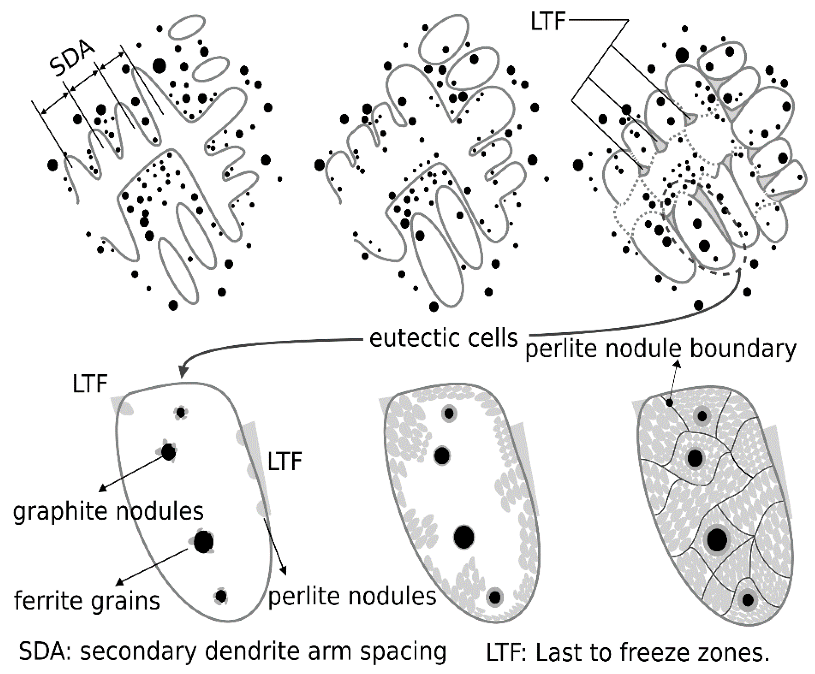
In the model that is introduced in the current work, the metastable eutectoid transformation is assumed to occur in two stages, as shown in Figure 2. The first step is the nucleation of the pearlite nodules and the second one is represented by the growth of these nodules. Each step is discussed in detail in the following sections.
2.1. Nucleation of Pearlite Nodules
Based on experimental observations, some authors have concluded that the pearlite colonies nucleate at the last to freeze (LTF) zones [12]. These regions are indicated in Figure 2 and represent the areas where some alloying elements (for instance, Mo, Mn, Cr and Ni) tend to segregate during the solidification. There are other authors who affirm that pearlite appears at the ferrite/austenite boundaries [13] without further evidence, i.e., without providing information about the crystallographic orientation relationship between ferrite growing in bulls-eye structure and the one present in pearlite.
In the current work, it is accepted that, as soon as the temperature reaches the upper limit of the three-phase field (), pearlite nucleation starts at the LTF zones, since pearlite is expected to be stable at temperatures lower than (Figure 1). Nevertheless, these nodules are only able to grow down .
In line with previous statements, the pearlite nucleation area is calculated based on the quantity and diameter of the eutectic cells. An estimation could be obtained from the experimental measurements developed by Rivera [12].
For modelling the nucleation, a continuous phenomenon was considered in agreement with Hull and Mehl [14] contributions, i.e., it was assumed that the saturation of the pearlite nucleation sites did not occur instantaneously during the cooling of the alloy. Then, continuous nucleation was assumed to be described by an Oldfield-type exponential nucleation law [15]. According to this model, the nucleation rate of pearlite colonies increases exponentially with the undercooling, as can be inferred from the following expression:
Taking into consideration that during continuous cooling the undercooling increases as the transformation progresses, the derivative of Equation (1) with respect to time allows contemplating the continuous nucleation of the perlite colonies as a function of the undercooling until the nucleation sites are saturated.
When calculating the derivative of Equation (1) with respect to time, the following expression is obtained:
where the superposed dot represents the temporal derivative of the variables, is the undercooling with respect to , n is a coefficient equal to 2 and is another coefficient whose value depends on the alloy chemical composition. In this article, was set to a value so that the density of pearlite colonies did not exceed the reference values published by Sorby and Mehl [16].
The upper limit of the three-phase field was calculated by making use of the expressions available in Appendix A, while the adopted values for y are indicated in Table A3.
In this new model, the pearlite nodules stop nucleating when the area covered by the pearlite nodules, which are represented by hemispheres, equals that corresponding to the eutectic cells obtained at the end of the solidification; or when recalescence occurs and the temperature is higher than the previous temperature, just in case austenite has not completely transformed.
From the previous paragraphs, it is clear that, if it is agreed that the pearlite nucleation occurs at the LTF zones, then the solidification outputs—in particular, the quantity and diameter of the eutectic cells—are of vital importance for modelling the pearlite reaction.
2.2. Growth of Pearlite Nodules
In accordance with the literature review, in this work, silicon partitioning between ferrite and cementite at the pearlite/austenite front was considered to rule the transformation. Among the expressions for pearlite growth rate as controlled by silicon partition, to the best of this author’s knowledge, Tewari and Sharma [5] have proposed the simplest one. It is based on the theory of growth of a lamellar eutectoid structure in a binary system [17] considering grain boundary diffusion. Therefore, the growth rate is:
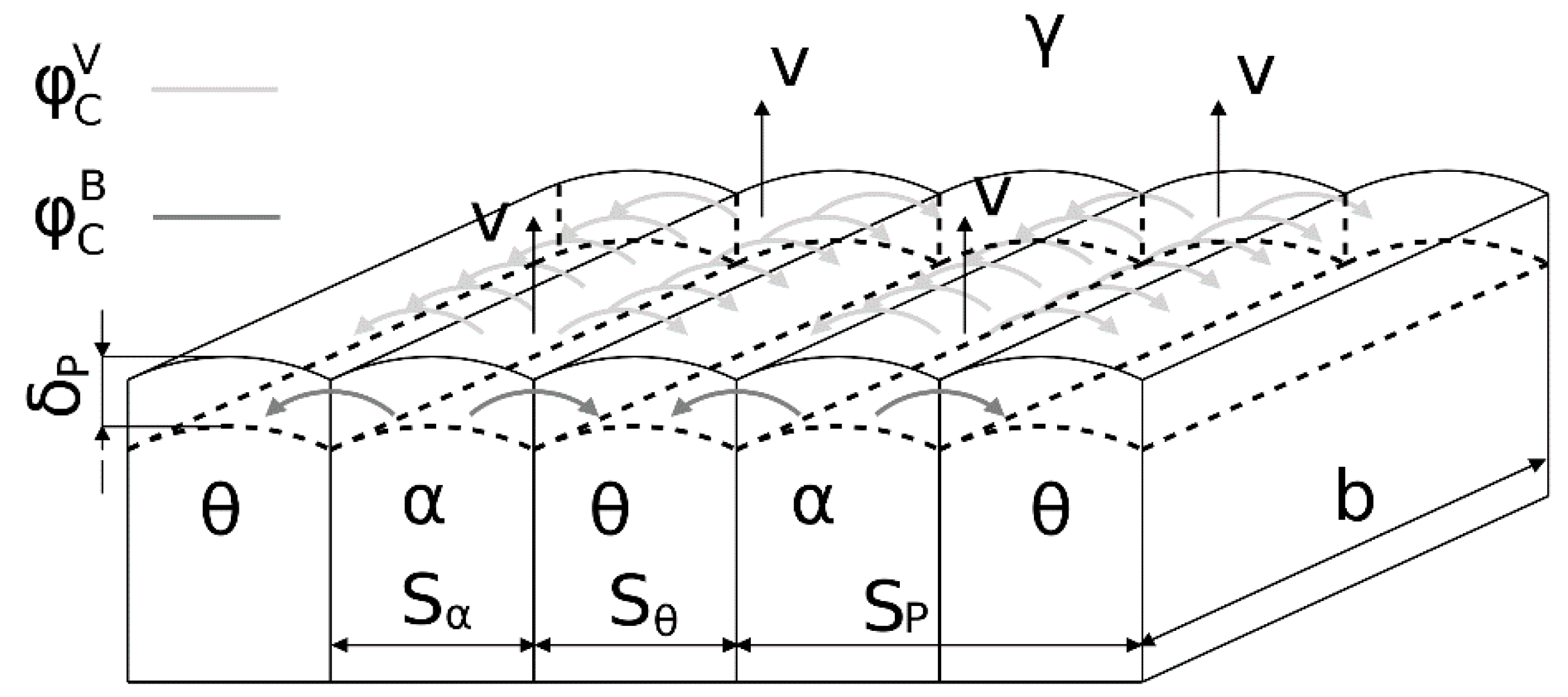
where represents the pearlite radius, k is the boundary segregation coefficient for silicon, is the interface diffusivity of silicon, is the boundary thickness, stands for the difference between the silicon equilibrium concentration at austenite in contact with ferrite and its equilibrium concentration at austenite in contact with cementite, denotes the average composition of silicon in the alloy, and SP is the interlamellar spacing (Figure 3).
At this point, it is important to define the term , since the microsegregation profiles inherited from the solidification step show clear differences in the silicon concentration among the different areas of the eutectic cell [18]. In this work, the silicon quantities registered at the LTF zones were considered, which are around 2 wt%-Si for the tested alloy [19]. This allowed, for the present analysis, to take the information of the driving forces directly from the calculations performed by Tewari and Sharma [5].
As stated in the previous section, the nucleated nodules were only able to grow down . For the tested alloy, the temperature, as calculated with the expressions given in Appendix A, was around 787 °C, close to the initial temperature of the experiments performed by Al-Salman et al. [4] and, therefore, the interlamellar spacing data was taken from their work. Other terms needed to perform the growing rate calculations making use of Equation (3) are available in Appendix B.
Once the radius variations of pearlite nodules were obtained for an integration time interval , the radius of a pearlite nodule i at an instant () is given by:
where is computed by incremental approximation of Equation (3).
After the radii of the pearlite nodules are available, the pearlite volume fraction can be calculated as:
where k is the number of events of nucleation of the pearlite nodules and is the number of pearlite nodules per unit volume associated with the i nucleation event.
Once the transformation of the austenite takes place, the austenite fraction should be computed again by the application of the following equation:
2.3. Application of the Model
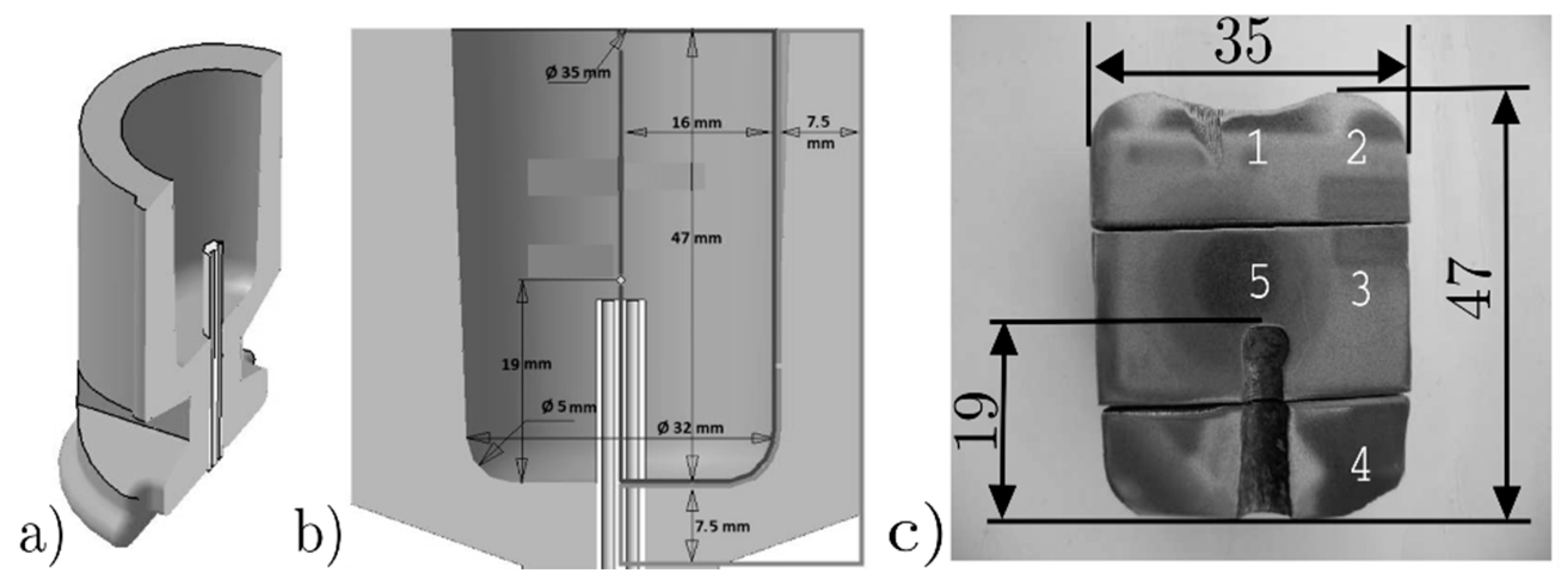
The model adopted in this paper has been used in the thermo-metallurgical simulation of the cooling of an SGI with a slightly hypereutectic composition (Table 1). The material was cast in a coupon with a circular cross-section of the type used to evaluate the equivalent carbon. A longitudinal section of the midplane of the specimen, together with a scheme of the coupon and the thermocouple, is shown in Figure 4.
The thermal history of the cooling process was recorded in the central zone of the specimen (zone 5 in Figure 4c). Nevertheless, all the zones indicated in Figure 4c were microstructurally characterized and all of them were considered in the metallurgical study for the measurement of the pearlite fractions. The casting process was repeated three times and three different recordings were registered [11].
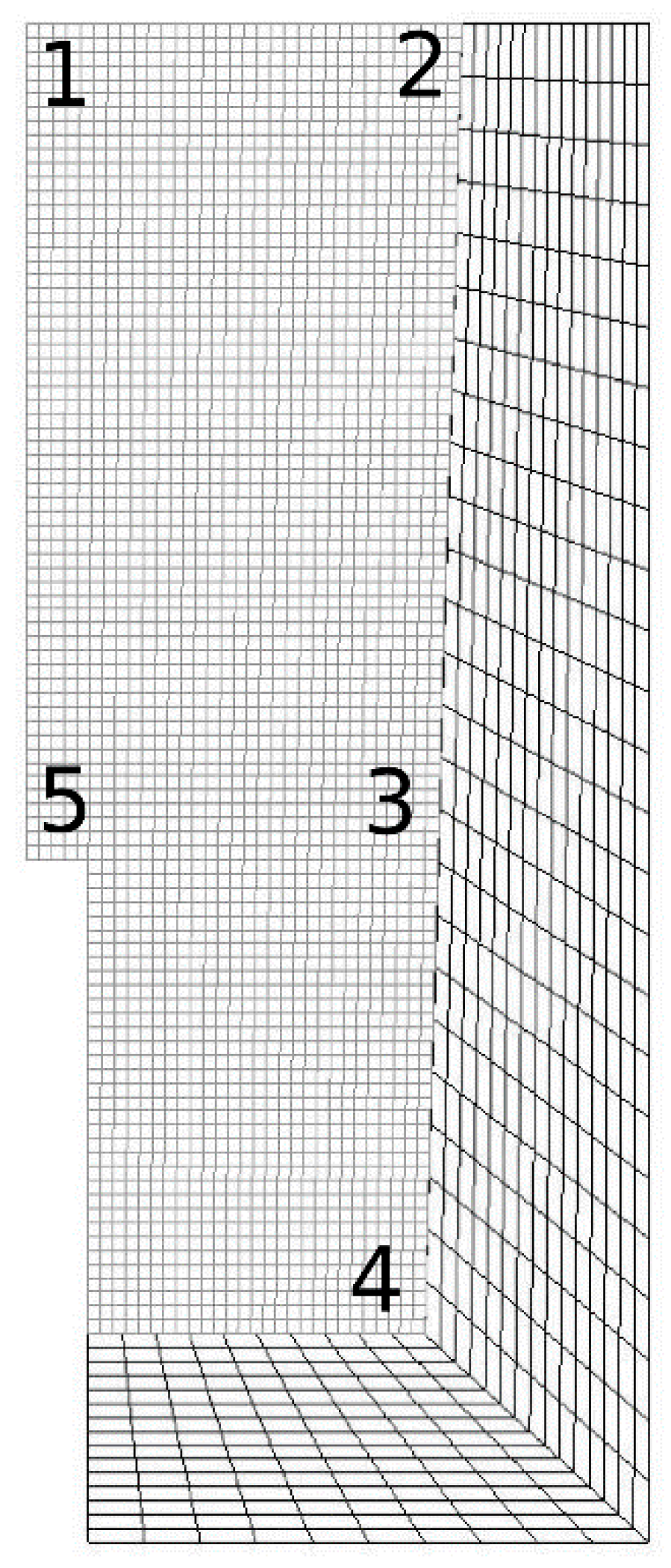
Due to the axial symmetry of the cup, only half of the longitudinal plane was discretized with quadrilateral four-node elements, using 2838 and 525 elements to represent the specimen and the mold, respectively. For each of the regions identified in Figure 4c, one node was studied. Each node was denominated making use of the same nomenclature as in Figure 4c, i.e., node 1 for zone 1 and so on (Figure 5).
Interface elements were used to simulate the heat flow between the cup and the specimen, whereas boundary elements were considered for dealing with the heat extraction through convection in those parts in contact with air at room temperature (the external surface of the cup and part of the specimen) [10,11].
All the thermo-physical properties, material parameters, coefficients, and parameters used in the numerical simulations are presented in Appendix C.
3. Results and Discussion
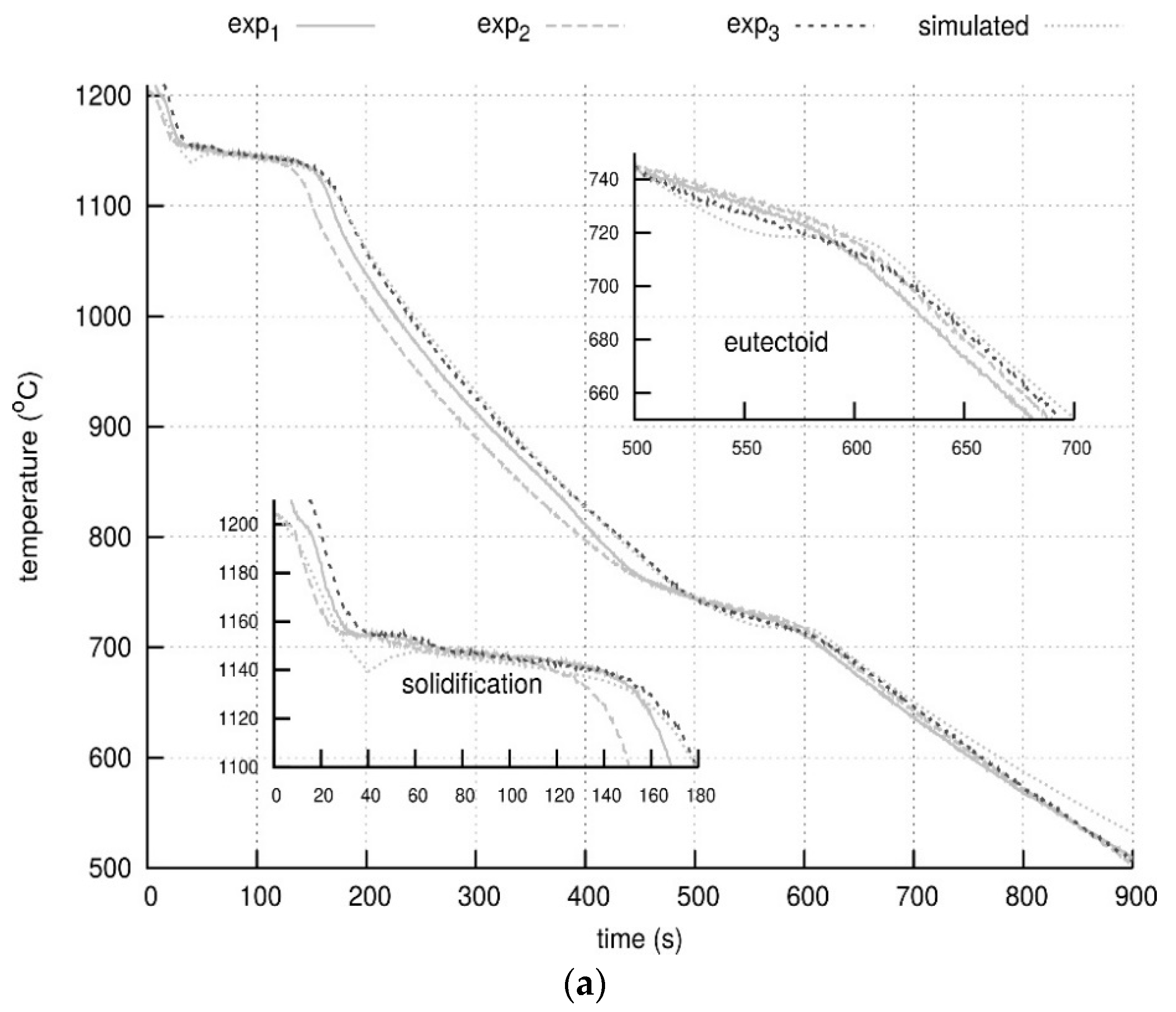
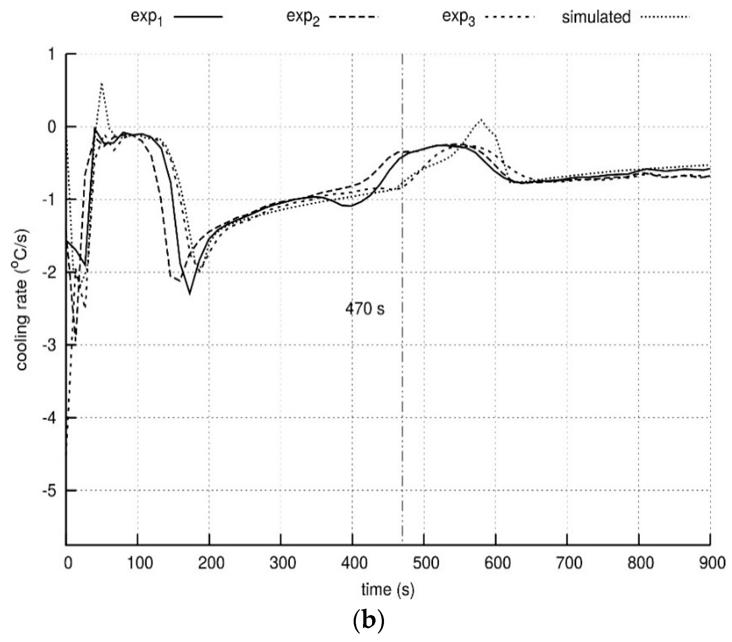
Computed cooling curves and cooling rate curves at the central region of the specimen are shown in Figure 6a,b, respectively. The computed cooling curves and cooling rate curves quantitatively agree with those corresponding to the three different experiments. In these figures, it can be seen that the metastable eutectoid transformation starts approximately at the same time in one of the experimental tests (exp3) and in the simulation: 470 s.
Comparing the region of the eutectoid transformation with the results reported in previous articles [10,11], in which pearlite reaction was modelled examining only the volume and the grain boundary diffusion of carbon in austenite, it can be seen that the present modelling results fit the experimental records more accurately.
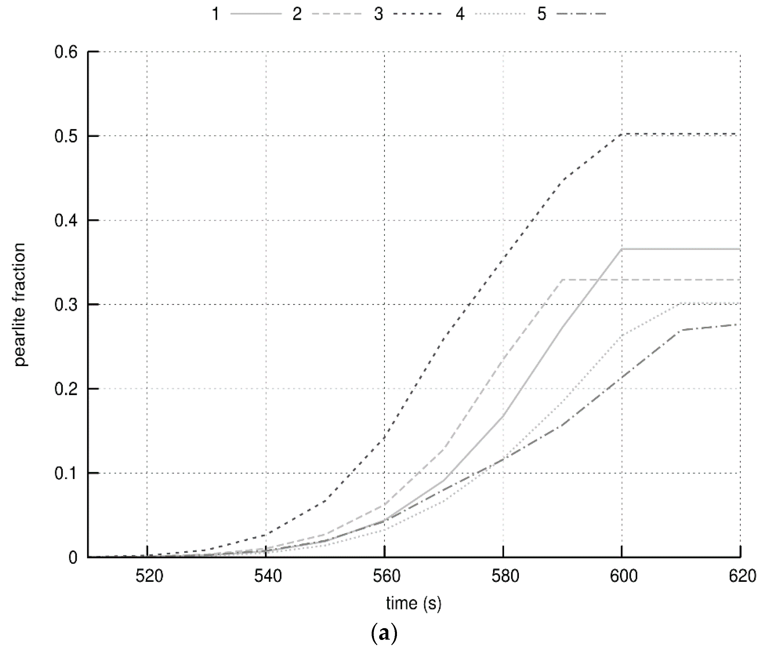
In Figure 7a, the simulated evolution of the pearlite volume fraction is shown for each of the studied zones. In this case, the time for the beginning of the metastable eutectoid transformation at node 3 was the shortest, while the temperature at which the decomposition of austenite to pearlite starts was the highest if compared with the nodes corresponding to the other four areas, i.e., nodes 1, 2, 4 and 5. The latter one presented similar pearlite fractions and transformation onsets. Indeed, the difference in the pearlite volume fractions was negligible for these four areas.
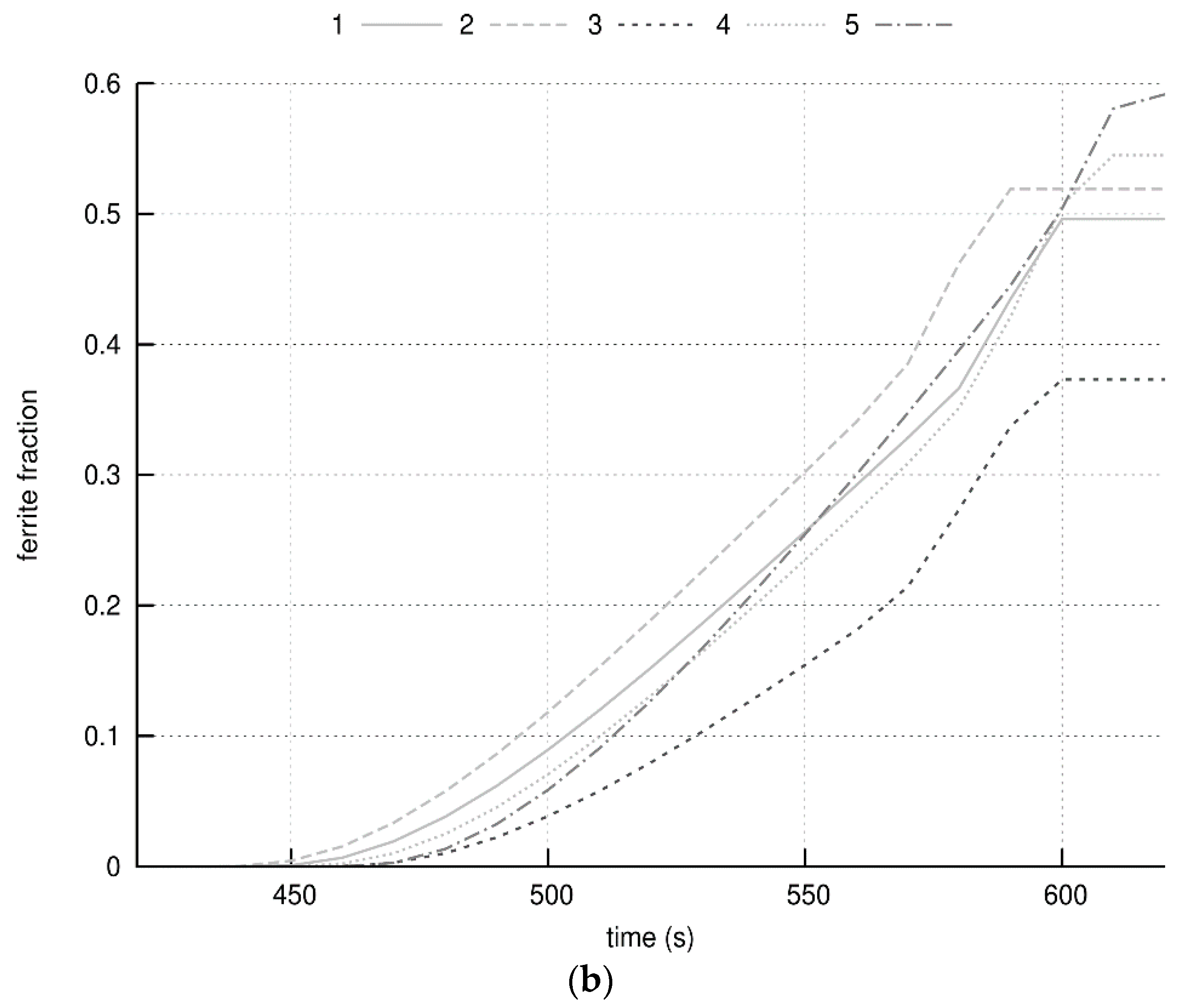
On the other hand, the calculated ferrite fractions presented in Figure 7b showed an inverse behavior compared to the pearlite fractions.
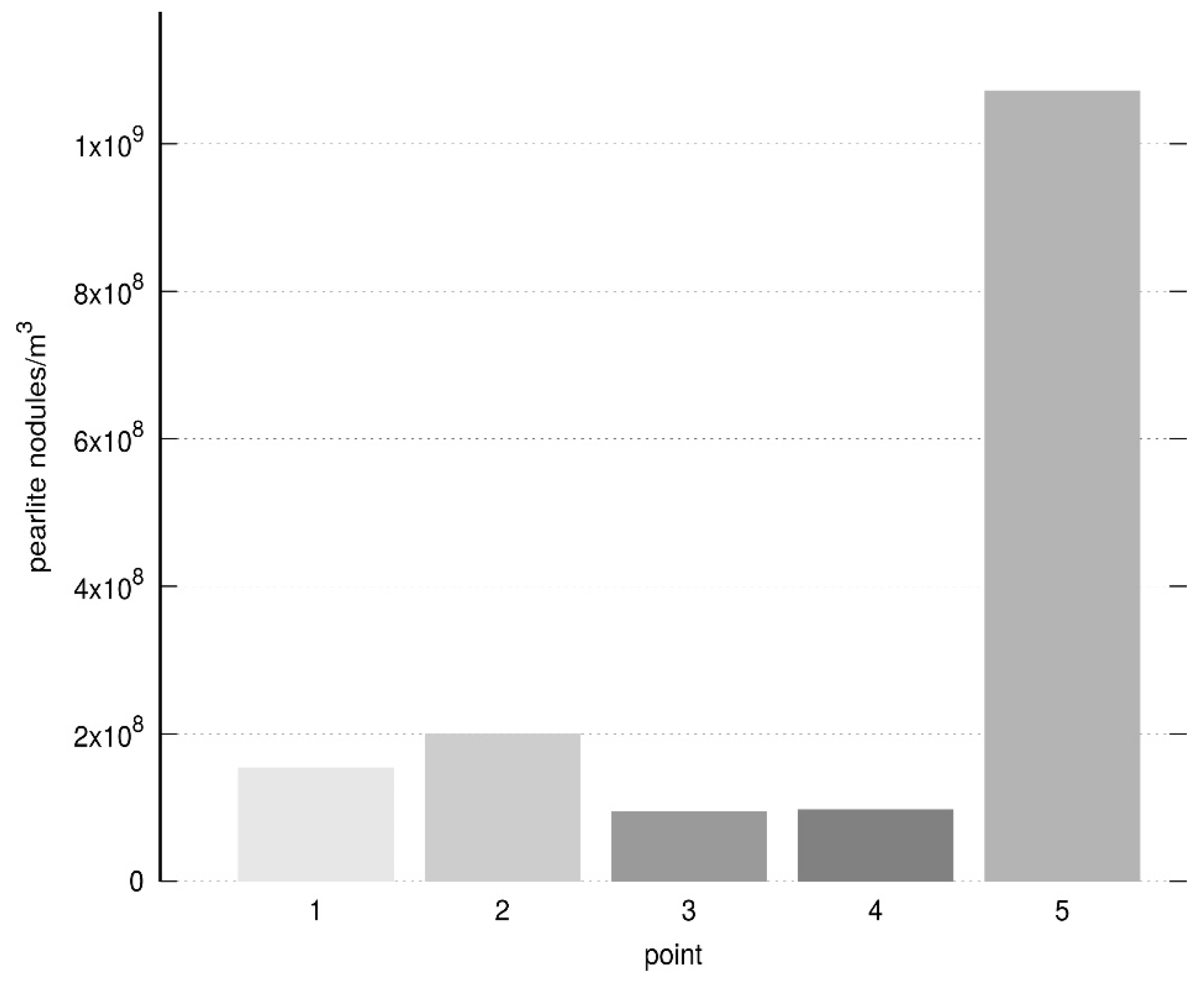
In Figure 8, the density of pearlite nodules per unit volume is plotted. Comparing Figure 7a and Figure 8, it is clear that the pearlite fraction obtained as the output of the simulation process did not have a direct relationship with the total density of pearlite nodules. In nodes 1, 2, 3 and 4, the nodule densities were of the same order, while in node 5 (central area of the specimen, next to the thermocouple), the density was considerably higher. If a ratio between the pearlite fraction and the nodule size distribution is recorded, it can be established that the zone with the highest pearlite fraction was the one with the highest percentage of large nodules, while the area that presents the lowest pearlite fraction was the one showing the lowest percentage of large nodules.
Unlike the previous work [10], where only the graphite fraction in the central region was calculated, in this paper, the graphite fractions were experimentally measured and compared with the calculated results for the five nodes; see Figure 9a. They showed good agreement. In Figure 9b, the simulated ferrite fractions confirm to fit the experimental results in four of the five areas. The ferrite fractions were of vital importance when simulating the pearlite transformation, as they were an indication of the austenite fraction that is available for decomposing into pearlite.
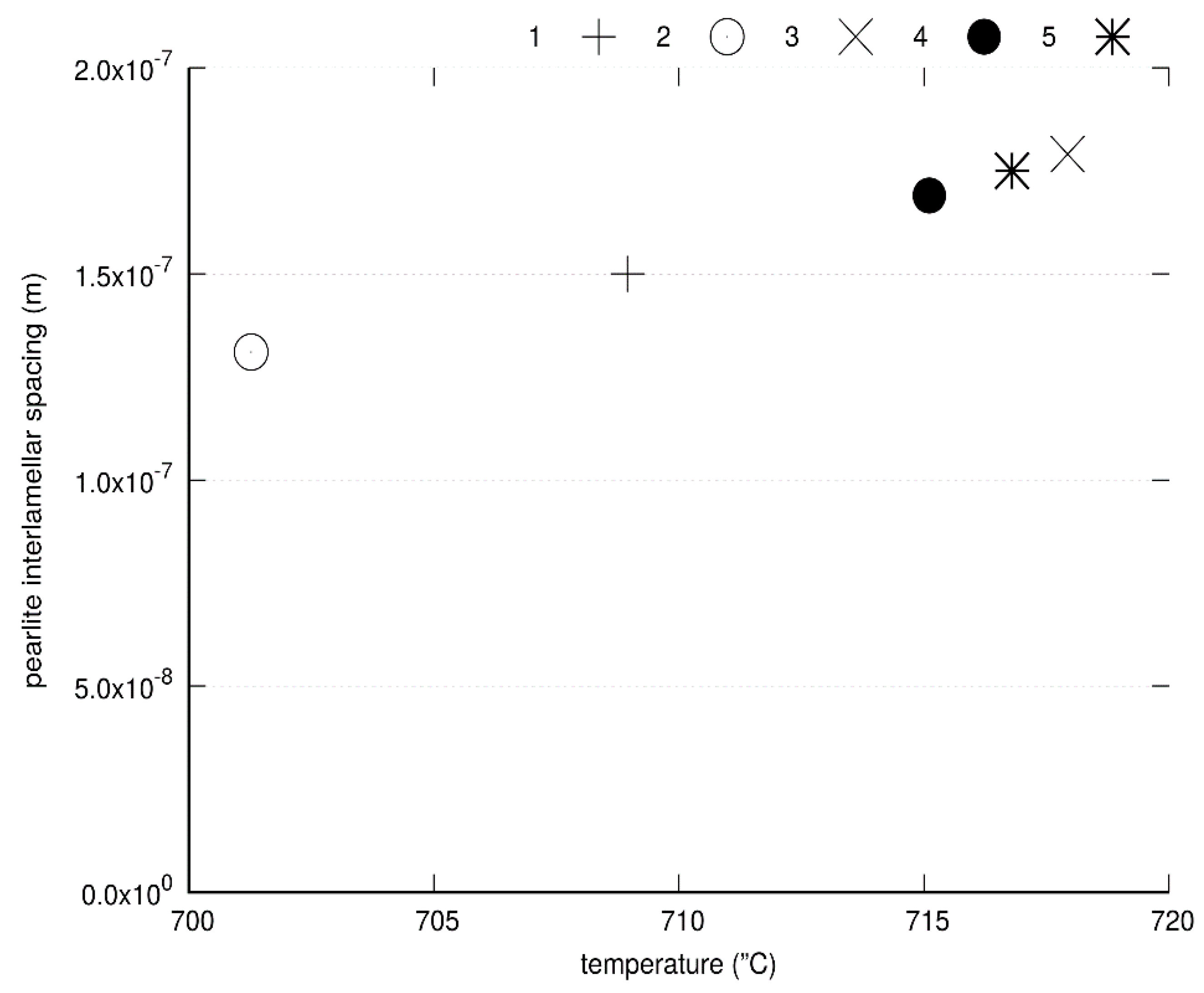
Later, the interlaminar spacing was calculated and plotted in Figure 10 at the end of the metastable transformation. As predicted by the theory, these measurements decreased as the undercooling increased.
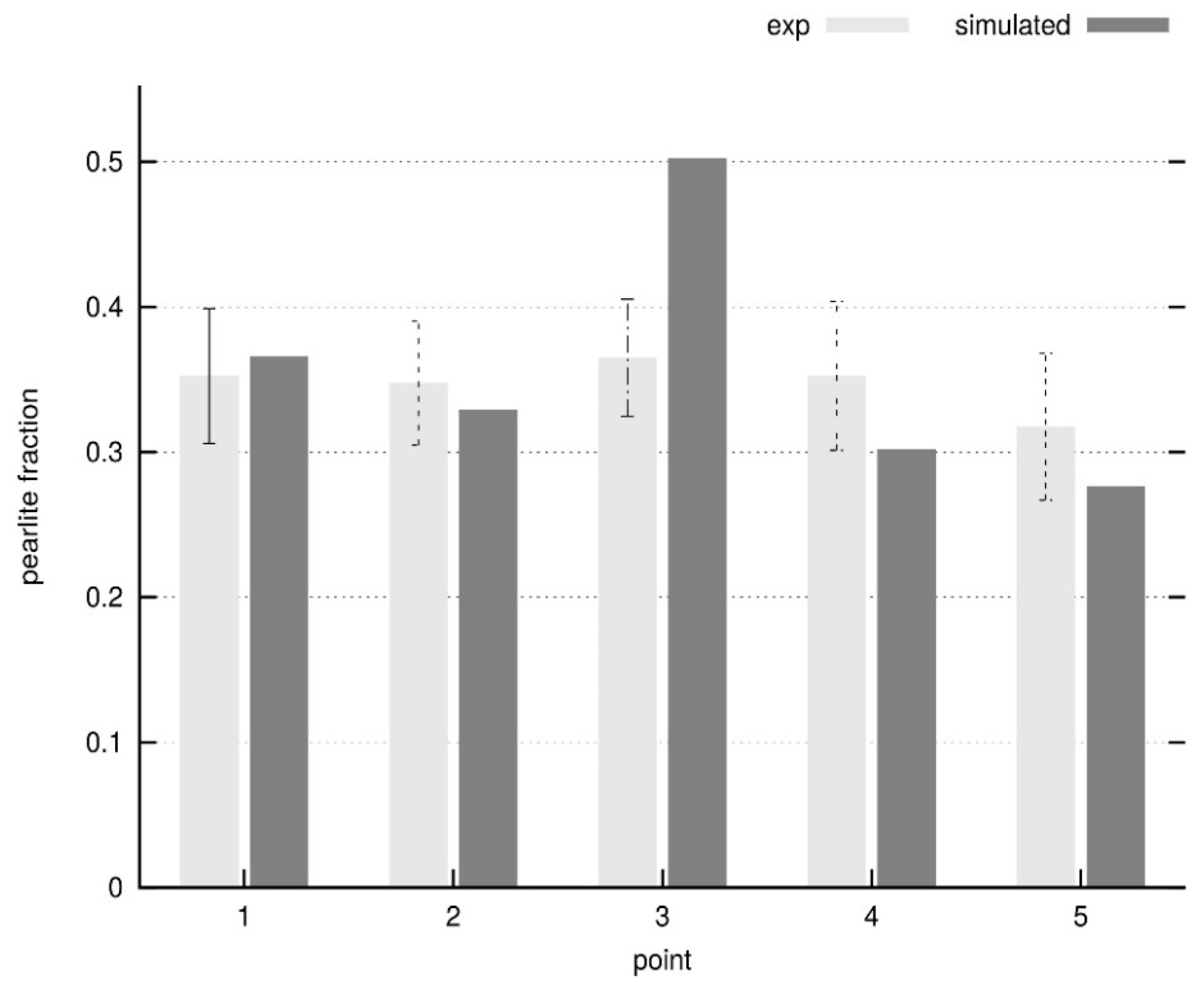
Finally, the experimentally measured and the calculated pearlite fractions were correlated as shown in Figure 11. Once more, they showed a good agreement except in the central area. On the other hand, concerning the experimental fractions, the difference between the maximum and minimum pearlite fractions was only 15.06%, whereas in case of simulated fractions—without taking into account the central node—the difference was 24%. In fact, these differences were within the expected standard deviations of the experimental results with respect to their mean value. As an example of the experimental measurement, a micrograph of the central section of the specimen is exposed in Figure 12. It was decided to append only one since the experimental measurements do not significantly vary from one point to another in the specimen (Figure 9 and Figure 11).
4. Conclusions
A new thermo-metallurgical model for simulating the metastable eutectoid transformation has been presented in this paper. In this model, the solidification stage, as well as the graphite growth and the stable eutectoid transformation have been all coupled and introduced as input for the metastable eutectoid transformation. Furthermore, silicon partition between ferrite and cementite at the austenite/pearlite interface has been assumed. The predictive ability of the model was evidenced by the accuracy between the experimental and simulated pearlite fractions for the low-alloyed SGI tested in this work.
Author Contributions
F.D.C. carried out the experimental test and the numerical simulations. F.D.C. and L.N.G proposed the model. F.D.C., L.N.G. and D.J.C. participated in the discussion of results and writing of the manuscript.
Funding
This research received no external funding.
Acknowledgments
The authors would like to thank the Sánchez and Piccioni company for allowing them to use its facilities to carry out the casts. F.D.C. and L.N.G. are members of CONICET (Argentinian Council of Research and Technology) and would like to thank the institution for the provided economic support. D.J.C. would like to thank CONICYT (Chilean Council of Research and Technology) for the support provided through the Project Fondecyt 1180591.
Conflicts of Interest
The authors declare no conflict of interest.
Appendix A. Critical Temperatures
The upper and lower limits of the three-phase field of the metastable Fe-C-Si diagram can be calculated by means of the following equations [11]:
where is the silicon content in austenite expressed in weight percentage and T is the temperature of the alloy in °C.
Appendix B. Nucleation Area, Silicon Concentration Differences, Interlamellar Spacing and Silicon Diffusivity at Pearlite/Austenite Interface
A total of 30 eutectic cells () was calculated per each austenite grain by analyzing the data provided by Rivera [12]. Then, the radius of the eutectic cell is given by:
The size of the austenite grain was calculated in a previous work [19]. Finally, the nucleation area can be calculated as:
where is the number of eutectic cells in the RVE (representative elementary volume).
The calculation of the difference between the silicon equilibrium concentration at austenite in contact with ferrite and its equilibrium concentration at austenite in contact with cementite, was obtained as a function of the temperature (°C) by fitting an equation to the data presented by Tewari and Sharma [5] for a 2 wt%-Si Fe-C-Si eutectoid alloy.
The interlamellar spacing at each temperature (°C) was found by a linear fit of the experimental values given by Al-Salman et al. [4]:
Appendix C. Thermo-Physical Properties and Material Parameters Adopted in the Numerical Simulations
Table A1, Table A2, Table A3 and Table A4 give information about the values of the coefficients and thermo-physical properties of the SGI and of the sand that were utilized in the numerical simulation [11,21]. Table A5, Table A6 and Table A7 present the data of the conductance and heat transfer coefficients at different interfaces of interest for the modeling. The alloy initial temperature is the same as the maximum value recorded in the experiments: 1205 °C [21]. The initial temperature for the cylindrical cup is the room temperature at the time the experiment was conducted: 20 °C.

Table A1.
Material parameters of SGI.
| Thermal Conductivity (W/mK) | Specific Heat (J/kg) | ||
|---|---|---|---|
| Temperature (°C) | Conductivity | Temperature (°C) | CP |
| 280 | 54.1 | 20 | |
| 420 | 38.1 | 600 | |
| 560 | 47.1 | 800 | |
| 700 | 43.6 | 1145 | |
| 840 | 38.1 | 1155 | |
| 980 | 32.5 | 1400 | |
| 1120 | 28.8 | - | - |
| 1400 | 45 | - | - |
| Mass density (kg/m3) | 7300 | - | - |
Table A2.
Thermo-physical properties of SGI: solidification phase change model [21].
Table A2.
Thermo-physical properties of SGI: solidification phase change model [21].
| Eutectic latent heat | (J/kg) | 2 105 |
| Carbon diffusion coefficient in liquid and austenite | (m2/s) | |
| Graphite nucleation coefficients | (grains/m3Ks) | |
| Graphite initial radius | (m) | |
| Austenite nucleation coefficient | (grains s/m3K) | |
| Gibbs-Thompson coefficient | (Km) | |
| Graphite and austenite densities | (kg/m3) |
Table A3.
Thermo-physical properties of SGI: solid-state phase change model.
| Initial thickness of the boundary layer ahead of the transformation front | (m) | |
| Ferrite latent heat | (J/kg) | |
| Initial number of ferrite grains | (grains) | |
| Initial radius of ferrite grains | (m) | |
| Pearlite latent heat | (J/kg) | |
| Pearlite nucleation coefficient | (grains s/m3K) |
Table A4.
Thermo-physical properties of the sand.
| Temperature (°C) | Thermal Conductivity (W/mK) |
|---|---|
| 100 | 0.54 |
| 300 | 0.57 |
| 500 | 0.65 |
| 700 | 0.79 |
| 900 | 1.00 |
| 1100 | 1.26 |
| 1300 | 1.59 |
| 1400 | 1.59 |
| Mass density (kg/m3) | 1550 |
| Specific heat (J/kg) |
Table A5.
Specimen-mold conductance coefficient.
| Temperature (°C) | Conductance Coefficient (W/m2K) |
|---|---|
| 20 | 60 |
| 500 | 70 |
| 850 | 90 |
| 1170 | 100 |
| 1400 | 100 |
Table A6.
Specimen-environment and mold-environment convection heat transfer coefficients.
| Temperature (°C) | Heat Transfer Coefficient (W/m2K) |
|---|---|
| 20 | 50 |
| 1400 | 80 |
Table A7.
Specimen-thermocouple conductance coefficient.
| Interface | Heat Transfer Coefficient (W/m2K) |
|---|---|
| Part-Thermocouple | 40 |
References
- Lacaze, J. GF G Pearlite growth in cast irons: A review of literature data. Int. Cast Met. Res. J. 1999, 11, 431–436. [Google Scholar] [CrossRef]
- Lacaze, J.; Wilson, C.; Bak, C. Experimental study of the eutectoid transformation in spheroidal graphite cast iron. Scand. J. Metall. 1994, 23, 151–163. [Google Scholar]
- Hillert, M. The mechanism of phase transformations in crystalline solid. Inst. Met. Monogr. 1969, 33, 231–247. [Google Scholar]
- Al-Salman, S.A.; Lorimer, G.W.; Ridley, N. Partitioning of silicon during pearlite growth in a eutectoid steel. Acta Metall. 1979, 27, 1391–1400. [Google Scholar] [CrossRef]
- Tewari, S.K.; Sharma, R.C. The effect of alloying elements on pearlite growth. Metall. Mater. Trans. A 1985, 16, 597–603. [Google Scholar] [CrossRef]
- Lacaze, J.; Gerval, V. Modelling of the eutectoid reaction in spheroidal graphite Fe-C-Si alloys. ISIJ Int. 1998, 38, 714–722. [Google Scholar] [CrossRef]
- Stefanescu, D.M.; Kanetkar, C.S. Computer Simulation of Microstructural Evolution; D. J. Srolovitz: Warrendale, PA, USA, 1985; pp. 171–188. [Google Scholar]
- Liu, B.C.; Zhao, H.D.; Liu, W.Y.; Wang, D.T.; Shangguan, D.; Cheng, J. Study of microstructure simulation of spheroidal graphite cast iron. Int. J. Cast Met. Res. 1999, 11, 471–476. [Google Scholar] [CrossRef]
- Almansour, A.; Matsugi, K.; Hatayama, T.; Yanagisawa, O. Simulating Solidification of Spheroidal Graphite Cast Iron of Fe–C–Si System. Mater. Trans. JIM 1995, 36, 1487–1495. [Google Scholar] [CrossRef]
- Carazo, F.D.; Dardati, P.M.; Celentano, D.J.; Godoy, L.A. Nucleation and growth of graphite in eutectic spheroidal cast iron: Modeling and testing. Metall. Mater. Trans. A 2016, 47, 2625–2641. [Google Scholar] [CrossRef]
- Carazo, F.D.; Dardati, P.M.; Celentano, D.J.; Godoy, L.A. Stable eutectoid transformation in nodular cast iron: Modeling and validation. Metall. Mater. Trans. A 2017, 48, 63–75. [Google Scholar] [CrossRef]
- Rivera, G. Estructura de Solidificación de Fundiciones de Hierro con Grafito Esferoidal. Ph.D. Thesis, Univesidad Nacional de Mar del Plata (INTEMA), Mar del Plata, Argentina, 2000. [Google Scholar]
- Roviglione, A.N.; Hermida, J.D. From flake to nodular: A new theory of morphological modification in gray cast iron. Metall. Mater. Trans. B 2004, 35, 313–330. [Google Scholar] [CrossRef]
- Hull, F.C.; Colton, R.A.; Mehl, R.F. Rate of nucleation and rate of growth of pearlite. Trans. AIME 1942, 150, 66–68. [Google Scholar]
- Oldfield, W. A quantitative approach to casting solidification, freezing of cast iron. Trans. Am. Soc. Met. 1966, 59, 945–961. [Google Scholar]
- Howell, P.R. The Pearlite Reaction in Steels Mechanisms and Crystallography: Part I. From H. C. Sorby to R. F. Mehl. Mater. Charact. 1998, 40, 227–260. [Google Scholar] [CrossRef]
- Fridberg, J.; Hillert, M. Ortho-pearlite in silicon steels. Acta Metall. 1970, 18, 1253–1260. [Google Scholar] [CrossRef]
- Boeri, R. The Solidification of Ductile Cast Iron. Ph.D. Thesis, The University of British Columbia, Vancouver, BC, Canada, 1989. [Google Scholar]
- Garcia, L.N.; Carazo, F.D.; Dardati, P.M. The transition from stable to metastable system and its relation with the ferrite halo extension in SG cast irons. Int. J. Cast Met. Res. 2017, in press. [Google Scholar] [CrossRef]
- Fridberg, J.; Torndahl, L.E.; Hillert, M. Diffusion in iron. Jernk. Ann. 1969, 153, 263–276. [Google Scholar]
- Dardati, P.M.; Godoy, L.A.; Celentano, D.J. Microstructural simulation of solidification process of spheroidal-graphite cast iron. J. Appl. Mech. 2006, 73, 977–983. [Google Scholar] [CrossRef]
Figure 1.
Fe-C binary isopleth section of the Fe-C-Si equilibrium phase diagram.

Figure 2.
Schematic representation of the nucleation and growth steps in pearlite transformation in spheroidal graphite cast irons (SGI) as assumed in the present model.
Figure 2.
Schematic representation of the nucleation and growth steps in pearlite transformation in spheroidal graphite cast irons (SGI) as assumed in the present model.

Figure 3.
Schematic representation of a growing pearlite colony.

Figure 4.
Sampling cup in which the molten metal was poured. (a) A 3D perspective of half section of the cup. (b) Front view of the cup with the thermocouple and the bifilar. (c) Longitudinal view of the specimen: its dimensions are indicated (in mm) and five zones numbered, which were microstructurally characterized.

Figure 5.
FE mesh of the specimen and mold used in the simulations. The location of the nodes, where the results were analyzed, are specified.
Figure 5.
FE mesh of the specimen and mold used in the simulations. The location of the nodes, where the results were analyzed, are specified.

Figure 6.
Comparison of experimental and simulated (a) cooling curves and (b) cooling rate curves, at the center of the specimen (zone 5). The solidification and eutectoid transformation zones are enlarged.
Figure 6.
Comparison of experimental and simulated (a) cooling curves and (b) cooling rate curves, at the center of the specimen (zone 5). The solidification and eutectoid transformation zones are enlarged.


Figure 7.
Simulated volume fractions of (a) pearlite and (b) ferrite as a function of time at each of the five regions.
Figure 7.
Simulated volume fractions of (a) pearlite and (b) ferrite as a function of time at each of the five regions.


Figure 8.
Simulated number of pearlite nodules per unit volume at each of the five regions.

Figure 9.
Experimental and simulated (a) graphite and (b) ferrite fractions at each of the five regions. Standard deviations for the experimental measurements are indicated.
Figure 9.
Experimental and simulated (a) graphite and (b) ferrite fractions at each of the five regions. Standard deviations for the experimental measurements are indicated.

Figure 10.
Simulated interlamellar spacing at the end of the metastable transformation at each of the five regions.
Figure 10.
Simulated interlamellar spacing at the end of the metastable transformation at each of the five regions.

Figure 11.
Experimental and simulated pearlite fraction per unit area at each of the five regions. Standard deviations for the experimental measurements are indicated.
Figure 11.
Experimental and simulated pearlite fraction per unit area at each of the five regions. Standard deviations for the experimental measurements are indicated.

Figure 12.
Micrograph of the central section of the specimen (100×).

Table 1.
Average chemical composition of the molten alloy (values in weight percentage).
| Element | C | Si | Mn | S | P | Cr | Cu | Sn | Mg | CE |
|---|---|---|---|---|---|---|---|---|---|---|
| wt% | 3.67 | 2.8 | 0.21 | 0.01 | 0.038 | 0.025 | 0.01 | 0.0009 | 0.052 | 4.61 |
© 2018 by the authors. Licensee MDPI, Basel, Switzerland. This article is an open access article distributed under the terms and conditions of the Creative Commons Attribution (CC BY) license (http://creativecommons.org/licenses/by/4.0/).
Share and Cite
MDPI and ACS Style
Carazo, F.D.; García, L.N.; Celentano, D.J. Metastable Eutectoid Transformation in Spheroidal Graphite Cast Iron: Modeling and Validation. Metals 2018, 8, 550. https://doi.org/10.3390/met8070550
AMA Style
Carazo FD, García LN, Celentano DJ. Metastable Eutectoid Transformation in Spheroidal Graphite Cast Iron: Modeling and Validation. Metals. 2018; 8(7):550. https://doi.org/10.3390/met8070550
Chicago/Turabian StyleCarazo, Fernando D., Laura N. García, and Diego J. Celentano. 2018. "Metastable Eutectoid Transformation in Spheroidal Graphite Cast Iron: Modeling and Validation" Metals 8, no. 7: 550. https://doi.org/10.3390/met8070550
Note that from the first issue of 2016, this journal uses article numbers instead of page numbers. See further details here.