Characteristics of Residual Stresses Generated by Induction Heating on Steel Plates

Graduate School of Engineering, Nagoya University, Furo-cho, Chikusa-ku, Nagoya 464-8603, Japan
*
Author to whom correspondence should be addressed.
Metals 2018, 8(1), 25; https://doi.org/10.3390/met8010025
Submission received: 28 November 2017
/
Revised: 21 December 2017
/
Accepted: 27 December 2017
/
Published: 1 January 2018
(This article belongs to the Special Issue Experimental Assessment of Residual Stress in Engineering Materials Components)
Abstract
:This paper presents experimental and numerical investigations on the characteristics of residual stresses generated by induction heating (IH) on 12 mm thick steel plates. IH at 250 °C and 350 °C provided high tensile residual stresses in the heating field but high compressive stresses away from the heating field. The double heating case generated higher compressive residual stresses—around 200 MPa—than the single heating case because of the superposition of the compressive residual stresses. It will be expected to improve the fatigue performance of welded joints when IH is applied for repair work on existing steel structural members susceptible to fatigue damage. Numerical simulation models for predicting residual stresses by IH were proposed by adopting the body heat flux input and the surface heat flux input. They will be beneficial for identifying the optimum heating conditions, such as the target temperature and the heating field, for applying IH to the actual repair work of the steel structural members.
1. Introduction
A tremendous number of steel structures have been constructed due to their substantial benefits for ease of construction, time saving, labor saving, flexible shapes, aesthetic, etc. However, along with the aging of infrastructures, steel structures, especially steel bridges, have deteriorated due to the effect of fatigue and corrosion [1,2,3]. For example, fatigue cracks promote and propagate to the base metals, eventually resulting in fatigue failure, whereas corrosion reduces the thickness of members, affecting the strength of the members. Consequently, maintenance and repair have become of critical importance for the civil engineering industry.
Fatigue cracks are mainly generated from welded joints because of a high stress concentration due to imperfections in the geometric weld profile and high tensile residual stress by localized heat input by welding. It is well-known that these two factors strongly affect fatigue crack initiation and propagation from welded joints. Therefore, a lot of research has been conducted for improving the fatigue performance of welded joints by several techniques.
For example, mechanical treatment methods, such as grinding and TIG (Tungsten Inert Gas welding) dressing, can improve the weld toe profile and reduce the stress concentration [4,5,6]. However, tensile residual stresses still remain because of the heat production in the treatment process [7]. These two methods are difficult to perform for narrow parts, and will need time and manpower if a long treatment length is required. On the other hand, the shot peening method and the high-frequency mechanical impact treatment (HFMI) method have been employed to improve fatigue strength. Both of them could produce a beneficial compressive residual stress for fatigue performance improvement [7,8,9,10]. However, it was found that these methods can only be used for thin layer treatment.
Aside from the mechanical treatment methods, thermal treatment methods, known as post-weld heat treatment (PWHT), have been applied for residual stress control. PWHT is commonly carried out in the factory by a large-scale furnace or a laboratory furnace to provide heat treatment to the structural members [11,12,13]. Thus, it is not possible to use PWHT with a large scale furnace for repair work on existing steel bridges at the site. Some researchers have applied a thermal treatment method suitable for localized heat treatment. Wang et al. [14] and Lin and Chou [15] investigated the effect of the line reheating method on residual stress control. This method is able to reduce the residual stress by generating a uniform temperature field, but it is difficult to control an open flame and to obtain the optimum heating condition.
It is worth noting that induction heating (IH) has been used for localized heat treatment in welded steel pipes to control tensile residual stresses [16,17,18]. Heat treatment with IH commonly is used for pipelines and pressure vessels, which are basically made of thick plates, and it is not generally applied to civil engineering structures, for example, steel bridges. Hence, there will be a need for studying and evaluating the effect of heat treatment with IH on relatively thin structures. Unlike the other heat sources, IH is a non-contact heating and rapid heating method, and metals are generally heated by producing electromagnetic waves through an induction coil. Moreover, it can provide high safety in the work since no open flame, such as that of a gas burner, is used. Therefore, in this study, IH was selected as a portable heat source that would be applicable to the localized heat treatment and repair work of existing steel bridges and complicated structures in the case of improving fatigue performance. Besides, it is expected that IH could be applied safely not only at workshops but also at sites.
The main objective of our research work is to investigate the basic applicability of IH on the residual stress control of steel structural members. It was expected that the proposed heat treatment with IH would heat abruptly and produce a new stress distribution pattern to control the residual stress distribution generated by welding. To achieve this objective, the characteristics of residual stress generated by IH on steel plates were investigated in this study. A series of numerically verified experiments was conducted on the very simple steel plates by applying IH. It is anticipated that IH could generate compressive residual stresses which would be of benefit for the improvement of fatigue performance.
2. Experiment
2.1. Test Specimens
2.2. Induction Heating on Test Specimens
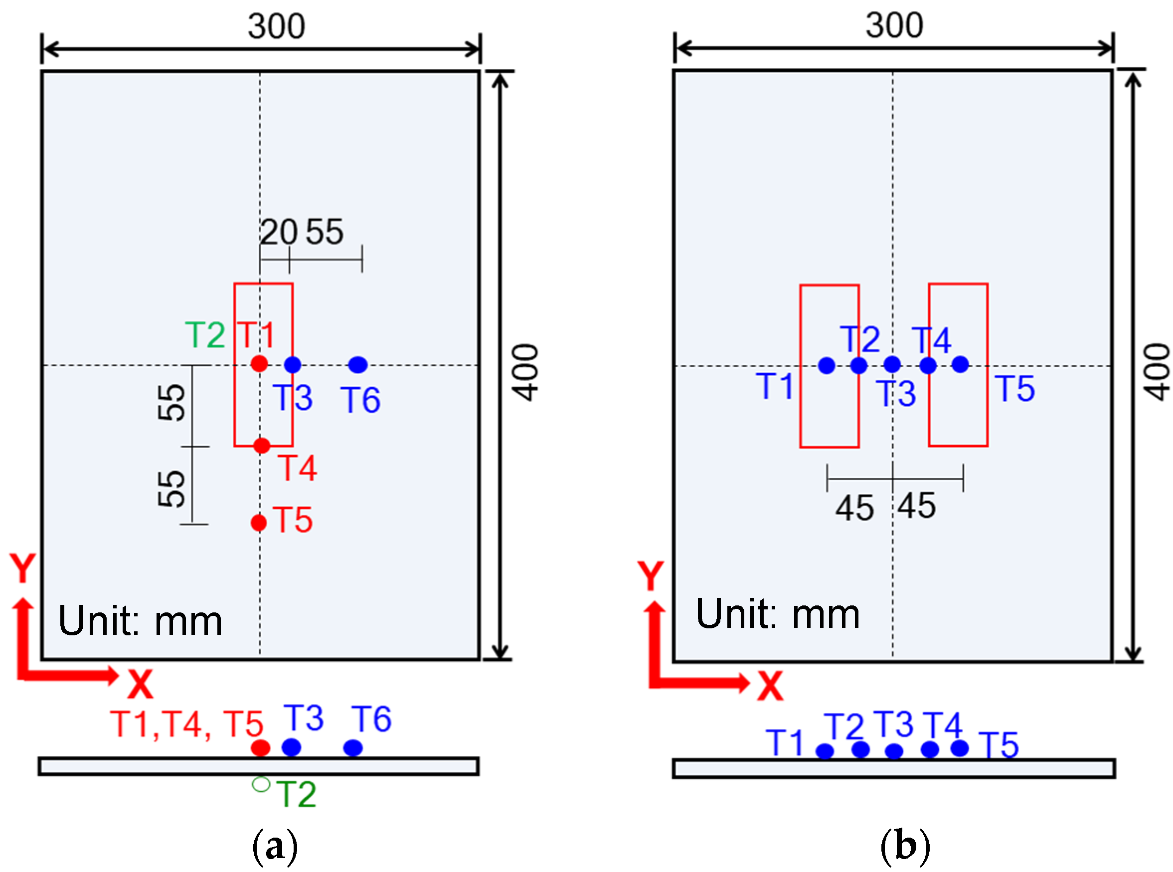
The size of the induction heating (IH) coil was selected as 40 × 110 mm. The current frequency was set as 28 kHz, and the heating field positions are shown in Figure 2. IH was applied only at the top surface of the specimens. Three cases of heating were carried out in order to evaluate the characteristics of the residual stresses generated by IH. Case 1 was the single heating case, and IH was applied at the center of the specimen with the target temperature of 250 °C. Case 2 and Case 3 were double heating cases, and IH was applied in one place after another but the target temperature was different. The adopted target temperatures were 250 °C for Case 2 and 350 °C for Case 3. The average power was 4.1 kW for Case 1 and 5.2 kW for Case 2 and Case 3. The main focus of this experiment is to control the target temperature. The temperature was monitored by the thermocouples attached to the specimens as depicted in Figure 3. When it reached the target temperature, the power was turned off.
There are certain reasons why these target temperature cases were selected. The mechanical properties of steel material are possibly changed when the steel is heated and the temperature reaches to a specified point, such as a transformation temperature. In order to prevent a change of mechanical properties of steel by IH in this study, the target temperature was decided to be lower than 400 °C. Furthermore, the relatively low temperature would be beneficial for safety in repair work on existing structural members.
2.3. Residual Stresses Measurement by the X-ray Diffraction Method
Before applying IH to the steel plates, annealing was performed with an electric furnace in order to release the initial residual stresses due to the manufacturing process. Specimens were soaked for about 5 h with the soaking temperature of 600 °C and cooled down gradually to ambient temperature. It was assumed that the annealing reduced the initial residual stress on the plate. Later, it was also proved that in the residual stress distribution of single heating (Figure 10), there was almost zero residual stress at the measurement points away from the heating field.
After applying IH, the residual stresses of the specimens were measured by applying the X-ray diffraction (XRD) method. The XRD method is a non-destructive method and measures a very thin layer surface to a depth of up to 30 μm. Strain is measured by the change of distances between crystal lattices from the X-ray diffraction angle. In the XRD method, the sin2Ψ and cosα methods are commonly used for residual stress measurement [19,20,21]. However, in this experiment, the cosα method was employed since it gives more reliable precision and accuracy of the stress measurement compared with the sin2Ψ method [20]. The parameters for XRD measurement are illustrated in Table 2.
Before the measurement, the surface of the specimens was grinded to remove weld used for thermocouples because the accuracy of XRD mainly depends on the condition of surface smoothness and grain size. Hence, it cannot measure at the welded points of the thermocouples, which has a coarse grain size. Residual stress measurements were made along the center line of a plate as depicted in Figure 4. A residual stress measurement was performed three times per point. It was confirmed that the standard deviation of the residual stresses was under 50 MPa.
3. Numerical Simulation
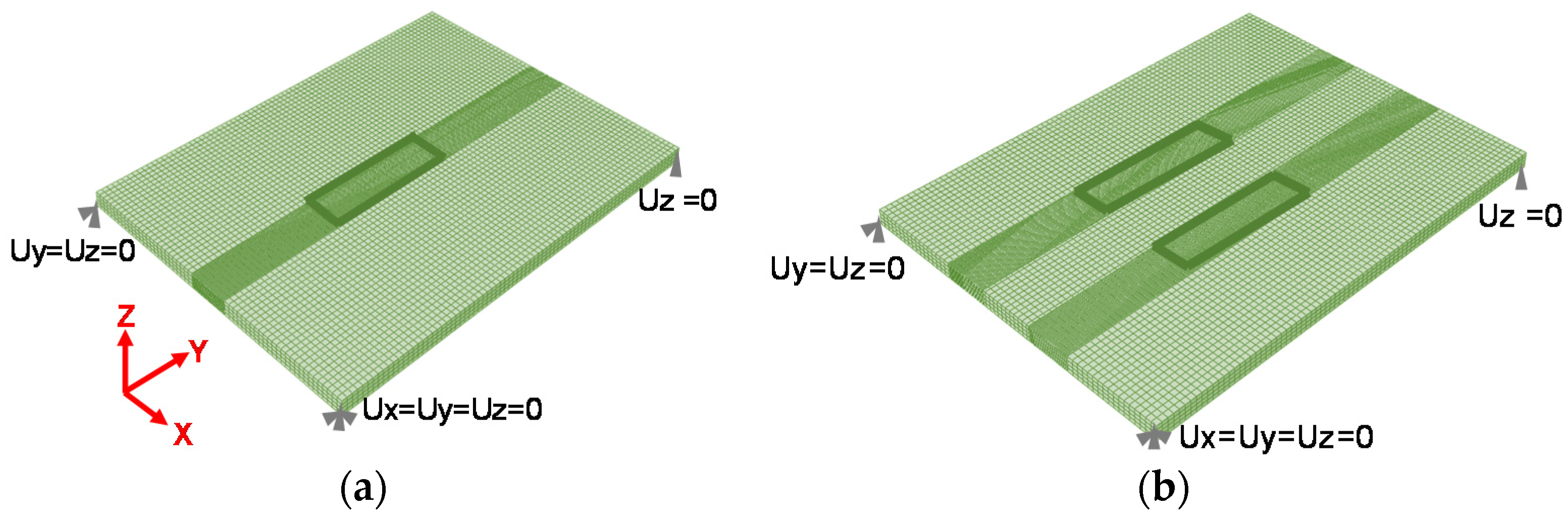
In order to investigate the tendency of the experimental results and develop the numerical simulation model for IH on relatively thin steel plates, a series of finite element analyses was carried out by using ABAQUS 6.14. The function of a coupled temperature-displacement analysis in the software was used. Eight-node linear brick elements (C3D8T) were employed for both the thermal and mechanical models, while elements were meshed with 1 × 5 mm at the heating field and 5 × 5 mm in the remaining area. Figure 5 represents the numerical models for the single and double heating cases. Temperature-dependent physical and mechanical properties were developed based on previous research [22,23] and are expressed in Figure 6.
For the thermal models, temperature-dependent physical properties (Figure 6a) were incorporated. Heat transfer from the surface of the model to the atmosphere due to natural convection and radiation was applied for the thermal boundary condition. For the initial temperature, the predefined ambient temperature (20 °C) was employed. The thermal models were constructed by employing two cases of heat input, such as the surface heat flux and the body heat flux, in order to examine which type of heat flux would provide better simulation results for IH.
The calculation of heat input for the numerical simulation was based on the average power supplied for IH. The average power from the electric power source was measured during the heating. Not all of the power was applied to the specimen because a part of it was consumed by the electric resistance and the temperature increase of the IH coil. Therefore, a thermal efficiency was adopted for the analysis. The magnitude of the heat input was decided to be the average power multiplied by the thermal efficiency. Furthermore, the heat input per unit area or per unit volume was obtained by dividing the heat input by the heating area or the heating volume achieved from the experiment.
For the surface heat flux model, the heat input was calculated by using Equation (1).
where, qS is the heat input (kJ/mm2), Q is the average power (kW), A is the area of heating field (mm2), and η is the thermal efficiency.
In the case of the body heat flux model, the heat input was predicted by using Equation (2).
Here, V is the volume of the heating field (mm3) and calculated by A × t, A is the area of the heating field (mm2), and t is the thickness of the specimen (mm). Up to now, almost no studies have been reported on the specific value of thermal efficiency for IH because the efficiency value for IH depends on the coil type, the electrical current through the induction coil, the frequency of the current, and the thermal properties and dimensions of the specimen. Therefore, in this study, the thermal efficiency was repeatedly analyzed and eventually it was set to 38%, which could reproduce a similar temperature history from the experiment for both the surface heat flux model and the body heat flux model.
Figure 6b shows the temperature-dependent mechanical properties that were input for the mechanical model. The nodal temperature from the thermal analysis was applied in the mechanical models. Mechanical boundary conditions were adopted in order to prevent rigid movement of the specimens as shown in Figure 5.
4. Results and Discussion
4.1. Temperature History
In order to investigate the influence of heating field positions and temperature on the residual stress state, three cases of heating conditions were implemented: single heating with the target temperature of 250 °C (Case 1), double heating with the target temperature of 250 °C (Case 2), and double heating with the target temperature of 350 °C (Case 3). For each case, numerical models were constructed with two different types of heat fluxes, the surface heat flux and the body heat flux, in order to examine which type of heat flux could provide better simulation results for the induction heating. Temperature distribution comparisons between the experimental results and the numerical simulations for each heating case are shown in Figure 7, Figure 8 and Figure 9.
4.1.1. Case 1: Single Heating (250 °C)
Figure 7 represents the temperature history for Case 1 (single heating with the target temperature of 250 °C). It took 69 s to reach the target temperature. The electric power for IH was switched off just after reaching the target temperature. Then, the specimen was naturally cooled down to the ambient temperature. Based on the thermocouples of T1 and T2 in the experimental investigation, which were installed at the center of the heating field of the top and bottom surfaces, the top and bottom surface temperatures were almost the same. Hence, it could be said that there was no temperature gradient through the thickness because the thickness of the specimen used in this study (12 mm) was relatively thin. The maximum temperature was observed at the center of the heating field, and as the distance from the center of the heating field increased, the more the temperature of the specimen decreased.
In the surface heat flux model shown by the dotted lines, the top surface temperature was higher than the bottom surface temperature. It might be because the surface heat flux was applied on the top surface of the model, and it might not distribute the temperature uniformly through the thickness of the model. The peak temperature at the center of the heating field from the experimental investigation was slightly lower than that from the surface heat flux model. However, there was a good agreement for the remaining parts between the experimental results and the numerical analysis.
On the other hand, compared to the surface heat flux model, the body heat flux model shown by the solid lines could generate more relevant temperature to the experimental results. In the body heat flux model, the top surface temperature coincided with the bottom surface temperature. It might be because the body heat flux could generate a uniform temperature to the top and bottom surfaces of the steel plate, and there might have been a symmetric temperature distribution through the thickness. There was excellent agreement between the experiment and the body heat flux model. Hence, it could be said that the body heat flux model was better than the surface heat flux model for the single heating case.
4.1.2. Case 2: Double Heating (250 °C)
In the double heating case, the specimen was heated firstly on the left side by applying IH until it reached the target temperature and then it was cooled down naturally to the ambient temperature. After the heating on the left side, the right side started to be heated, and was subsequently cooled down to the ambient temperature. The target temperature of Case 2 was 250 °C, and the duration to reach the target temperature was about 39 s for each side. Compared with the single heating case, the duration to reach the target temperature is shorter in this case. The reason might be that the current power for the single heating case was set as 4.1 kW, but in Case 2 it was increased to 5.2 kW. Hence, the Case 2 double heating reduced the heating duration from 69 s to 39 s although the same target temperature was applied. The temperature history for Case 2 is expressed in Figure 8. Similar to Case 1 (single heating), the maximum temperature was observed at the center point of both heating fields and reduced away from the center of the heating fields.
During the analysis steps, an application of heat on the right side was commenced after the left side heating field was heated to the target temperature and cooled down to the ambient temperature. The surface heat flux model produced a higher temperature than the experimental result as well as the body heat flux model. It was assumed that when applying surface heat flux on the top surface of the model, a non-uniform temperature distribution might be generated in the thickness direction.
Similar to the Case 1 single heating model, the temperature of the double heating case with the body heat flux almost coincided with the experimental results. Although the temperature of the numerical model in some points was slightly higher than that of the experimental results, it was not significant. Hence, it was noted that the body heat flux models could provide better agreement with the experimental results of the double heating case.
4.1.3. Case 3: Double Heating (350 °C)
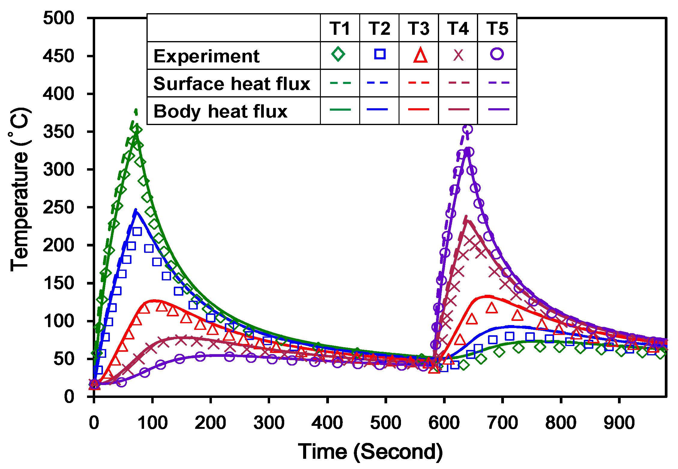
Case 3 was the double heating with a target temperature of 350 °C case. The purpose of applying a different temperature from Case 2 was that the effect of a different temperature on residual stress distribution was to be examined. The heating process and the heating field locations were the same as the Case 2 double heating case except for the target temperature and duration. The duration for Case 3 to achieve the target temperature was about 72 s. The temperature history for Case 3 is presented in Figure 9.
The maximum temperature generated by the surface heat flux model of Case 3 was slightly higher than that from the experiment, but the difference was not noticeable. Similarly, it produced a slightly higher temperature than the experiment during the heating stage, whereas the same temperature was observed during the cooling stage. However, good agreement between the experiment and the surface heat flux model was observed.
It was noticed that the temperature distribution from the body heat flux model in Case 3 almost coincided with that from the experiment except for some points. The body heat flux model produced a lower temperature at the center of the heating field than the surface heat flux model during the heating stage. However, the temperature distributions from both the surface and the body heat flux models almost coincided at other locations.
A larger heat input was applied in Case 3 than that applied in Case 2. Although the surface heat flux model generated the temperature distribution through the thickness in Case 3, the large heat input on the top surface might quickly reach the bottom surface. Therefore, the temperature difference between the top and bottom surfaces by the surface heat flux model of Case 3 might be smaller than that of Case 2. In other words, there was little difference between the surface heat flux and the body heat flux models in Case 3.
As a summary, the surface heat flux models for all cases generated a higher temperature than the experiment during the heating stage. In contrast, the body heat flux models accurately reproduced the temperature distribution of the experiment. Therefore, it could be concluded that the body heat flux provided better agreement with the experiment than the surface heat flux for simulating IH on 12 mm thick steel plates.
4.2. Residual Stresses
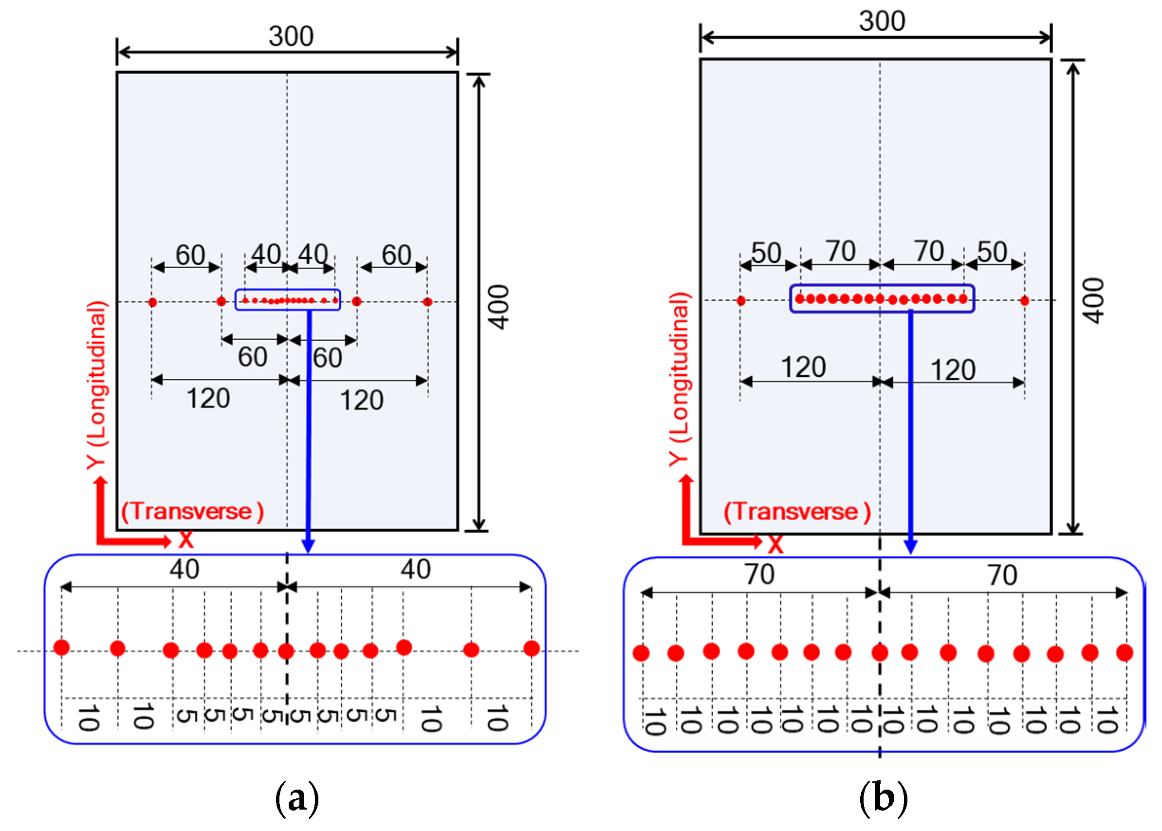
The XRD method was applied to measure the residual stresses in the experiment. The residual stress measurement was conducted at the center line of the top and bottom surfaces of the specimens along the direction of 300 mm width (Figure 4). Measured points were selected not only at the heating field area but also the outside of the heating field. As shown in Figure 4, the X-direction was defined as the transverse direction while the Y-direction was assumed to be the longitudinal direction. During the application of IH on the specimens, the center of the heating field experienced the highest temperature. Hence, both longitudinal and transverse tensile residual stresses were generated at the heating field position whereas compressive residual stresses were observed next to the heating field area in the longitudinal direction for balancing with the longitudinal tensile stresses (Figure 10, Figure 11 and Figure 12). The middle part between the two heating fields of Case 2 and Case 3 (double heating) experienced large compressive stresses because the compressive stresses were superimposed on the original tensile stress fields around there.
4.2.1. Case 1: Single Heating (250 °C)
In the single heating case, the residual stress patterns of the experiment and numerical simulations were similar in both the longitudinal and transverse directions, but their magnitudes were slightly different (Figure 10a,b). The reason might be the fact that the XRD method is delicate and the accuracy of it depends on the surface condition of the specimens. From the XRD measurement, the top surface residual stresses were slightly higher than the bottom surface residual stresses in both the longitudinal and transverse directions. It was found that the maximum tensile and compressive longitudinal residual stresses at the top surface were about 152 MPa and 124 MPa, respectively, while maximum tensile residual stresses of about 94 MPa and compressive residual stresses of about 144 MPa were observed at the bottom surface.
The maximum longitudinal residual stresses of the surface heat flux model were significantly higher than those from the experiment. The body heat flux model produced a symmetric stress distribution through the thickness. Therefore, the stresses on the top and bottom surfaces were the same. The result from the analysis of the body heat flux model is represented by only one black solid line. As shown in Figure 10a, the residual stresses at the top surface of the surface heat flux model were relatively higher than those induced by the body heat flux model, whereas the bottom surface residual stresses of the surface heat flux model were lower than the residual stresses of the body heat flux model. This was due to the fact that surface heat flux model in the single heating case generated a higher temperature than the experiment (Figure 7). The surface heat flux model induced a maximum tensile residual stress of about 235 MPa and a maximum compressive residual stress of about 92 MPa, while a maximum tensile residual stress of 166 MPa and a compressive stress of 77 MPa were found in the body heat flux model. The stresses obtained by the body heat flux model were relatively closer to the XRD measurement results rather than the stresses obtained by the surface heat flux model.
The XRD measurement showed that the transverse residual stresses at the top surface were higher than those at the bottom surface except at some points (Figure 10b). The maximum transverse residual stresses at the top and bottom surfaces were about 84 MPa and 63 MPa in tension, respectively, and 35 MPa and 89 MPa in compression, respectively. However, both the surface heat flux model and the body heat flux model induced less transverse residual stresses than the XRD measurement in both tension and compression. The surface heat flux model generated slightly higher transverse residual stresses than the body heat flux model, but the difference was not remarkable. However, it was found that the compressive transverse residual stresses produced by both models were considerably smaller than the experimental results. This might be that there was an error or inaccuracy at some points from which the high compressive stresses were obtained in the XRD measurements.
4.2.2. Case 2: Double Heating (250 °C)
In Case 2 (double heating), the longitudinal and transverse residual stresses at the top and bottom surfaces were very similar (Figure 11a,b). Similar to the single heating case, the residual stress patterns measured by XRD were similar to that by the surface heat flux model and the body heat flux model although their magnitudes were not the same. It was obvious that Case 2 (double heating) induced lower tensile and compressive residual stresses of about 132 MPa and 118 MPa, respectively, compared with the Case 1 single heating model, although the same target temperature (250 °C) was applied to both models. The reason might be that IH was applied to the right side after completing the left side heating process, and consequently the later heating process might act as a stress reduction on the earlier heating process.
Similar to Case 1, the surface heat flux model generated higher longitudinal residual stresses at the top surface than the experiment and the body heat flux model, while relatively higher residual stresses at the top and bottom surface were observed in the experiment compared with the body heat flux model (Figure 11a).
Dealing with the residual stresses in the transverse direction, relatively higher transverse residual stresses were experienced in the XRD measurement than in the numerical models, especially in tension (Figure 11b). However, the transverse residual stresses in both the top and bottom surfaces were almost the same in not only the experiment but also the numerical models. Therefore, it was noted in this case that the numerical models could simulate a similar tendency of the transverse residual stresses but the difference in magnitude was not small.
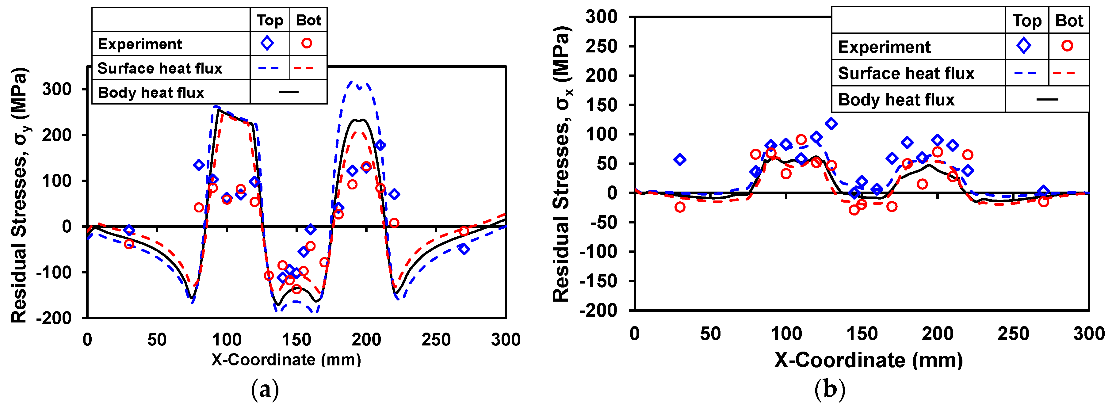
4.2.3. Case 3: Double Heating (350 °C)
When increasing the target temperature, the Case 3 double heating model induced high compressive longitudinal residual stresses, with about 136 MPa from XRD, 170 MPa from the body heat flux model, and 192 MPa from the surface heat flux model (Figure 12a), which were much higher than those generated by the Case 2 model. Dissimilar to Case 1 and Case 2, the longitudinal residual stresses at the top and bottom surfaces induced by the surface heat flux model were almost the same as those by the body heat flux model at the left side heating field. However, at the right side heating field, the top surface residual stresses produced by the surface heat flux model were relatively higher than those by the body heat flux model. It was noted that the longitudinal residual stresses from the numerical models were much closer to the XRD measurement when a higher target temperature was set. It might be that the later heating process might act as a stress reduction on the earlier heating process. In other words, the residual stresses generated by the earlier heating process were redistributed by the later heating process. The influence of it might be larger in Case 3 than that in Case 2.
In the case of the transverse residual stresses, the residual stresses at the top surface were slightly higher than those at the bottom surface in the XRD measurement (Figure 12b). The numerical models for the Case 3 double heating model with the target temperature of 350 °C could predict the XRD measurement well compared to Case 1 and Case 2.
In summary, the surface heat flux models for all cases overestimated the residual stresses at the tension side of the top surface while the residual stresses at the bottom surface were closed to the experiment. However, the residual stresses from the body heat flux models were much closer to those from the experiment. Case 1 induced higher residual stresses than Case 2, although the same target temperature was applied. Based on the XRD results, the double heating with 250 °C induced the maximum compressive residual stresses of about 120 MPa, but when the temperature was increased, the compressive residual stresses were raised to 136 MPa. It was also noted that not only the target temperature but also the heating field positions influenced the magnitude of the residual stresses.
In any case, the possibility of controlling the residual stresses in steel plates by IH with a relatively low temperature and quick duration could be confirmed. Furthermore, an analytical method for prediction of the residual stress distribution could be developed. The residual stress control by IH is expected to improve the performance of steel structural members. That is, the fatigue strength of a welded joint, which is strongly influenced by welding tensile residual stresses, may be improved by applying IH around the welded part and converting the tensile stresses to compressive stresses. This kind of performance improvement of steel structural members will be intended to be applied in future works.
5. Conclusions
A fundamental investigation on simple steel plates was conducted to evaluate the characteristics of residual stresses generated by induction heating (IH) with a relatively low temperature. The following conclusions can be made for this study:
- The temperatures 250 °C and 350 °C of IH on the top surface of 12 mm thick steel plates generated little temperature gradient through the thickness.
- Case 1 and Case 2 heat treatments were performed with the target temperature of 250 °C. The Case 1 heat treatment was conducted by 4.1 kW of current power and it took about 69 s to reach the target temperature. However, in Case 2, current supply was increased to 5.2 kW and the duration was about 39 s to reach the target temperature. It was noted that heat treatment with IH made it possible to achieve the same target temperature in a shorter time, resulting in economic benefit due to energy saving.
- In the longitudinal direction, single heating to 250 °C generated the maximum tensile residual stresses of 152 MPa at the top surface and 94 MPa at the bottom surface of the heating field, whereas the compressive residual stresses were about 124 MPa at the top surface and 144 MPa at the bottom surface for balancing the tensile residual stresses.
- Double heating to 250 °C produced the maximum tensile residual stress of 132 MPa and the maximum compressive stress of 120 MPa. Since the second heating acted as the stress release on the first heating process, the residual stresses of the double heating were lower than those of the single heating with the same temperature.
- Double heating to 350 °C induced the maximum tensile residual stress of 178 MPa and the maximum compressive stress of 136 MPa. The residual stress control by IH is expected to improve the performance of steel structural members. If this compressive stress is superimposed on the tensile residual stress around the welded part, then the fatigue performance of the welded part is expected to be improved.
- Heat input for the heat treatment was incorporated into numerical models based on the experimental data. Since two different power supplies, for example 4.1 kW for single heating and 5.2 kW for double heating, were adopted for the heat treatment, heat inputs were not the same even though the target temperatures were the same. However, heat treatment with IH provided a uniform thermal efficiency (38%), which could reproduce the temperature history from the experiment for all cases.
- The temperature histories by IH were more accurately simulated by the thermal condition analysis with the body heat flux input model than with the surface heat flux model. Besides that, the residual stresses generated by IH could be simulated by the thermo-mechanical analysis. The simulation accuracy of the body heat flux input model was relatively higher than that of the surface heat flux input model in this study using 12 mm thick steel plates. However, the simulation accuracy for the magnitude of the residual stress should be improved.
In future, it is anticipated that IH could be applied for the fatigue performance improvement of welded joints. The target temperature and heating field positions play important roles in achieving the designated position and magnitude of the compressive residual stresses. Therefore, further investigations should be carried out to find the heating field positions in order to obtain the optimum conditions for the application of IH in the fatigue performance improvement of welded joints. Then, the residual stress prediction procedure developed in this study will be beneficial for the investigation of fatigue performance improvement in welded joints.
Acknowledgments
A part of this research was supported by JSPS KAKENHI Grant Number 16H06098. The PWHT experiment was supported by JEMIX Co. Ltd and the XRD measurement was supported by Pulstec Industrial Co. Ltd.
Author Contributions
Mikihito Hirohata planned and managed this research totally. Masaaki Nakamura arranged the experimental conditions. May Phyo Aung was performed numerical simulation. They performed the experiment supported by JEMIX Co. Ltd and Pulstec Industorial Co. Ltd. May phyo Aung wrote this paper and Mikihito Hirohata checked and modified the paper.
Conflicts of Interest
The authors declare no conflict of interest.
References
- Tamakoshi, T.; Yokoi, Y.; Ishio, M. The feature of degradation of steel highway bridges estimated from the periodic inspection data collected out of Japan. Steel Constr. Eng. 2014, 21, 99–113. (In Japanese) [Google Scholar]
- Tanaka, Y.; Murakoshi, J. Evaluation and mitigation methods of corrosive environment around expansion joints of highway bridges. Civil. Eng. J. 2008, 50, 16–19. (In Japanese) [Google Scholar]
- Haghani, R.; Al-Emrani, M.; Heshmati, M. Fatigue-prone details in steel bridges. Buildings 2012, 2, 456–476. [Google Scholar] [CrossRef]
- Pedersen, M.M.; Mouritsen, O.Ø.; Hansen, M.R.; Andersen, J.G.; Wenderby, J. Comparison of post weld treatment of high strength steel welded joints in medium cycle fatigue. Weld. World 2010, 54, R208–R217. [Google Scholar] [CrossRef]
- Haagensen, P.J.; Maddox, S.J. IIW Recommendation on Post Weld Improvement of Steel and Aluminium Structures; IIW Doc. XIII-1815-00; International Institute of Welding: Roissy, France, 2003. [Google Scholar]
- Garud, V.; Bhoite, S.; Ingale, S.; More, S.; Lakade, S.S.; Matekar, S.B. Effect of post weld toe treatments on fatigue life of welded structures using FEA. Mater. Today Proc. 2017, 4, 1116–1126. [Google Scholar] [CrossRef]
- Cheng, X.; Fisher, J.W.; Prask, H.J.; Gnäupel-Herold, T.; Yen, B.T.; Roy, S. Residual stress modification by post-weld treatment and its beneficial effect on fatigue strength of welded structures. Int. J. Fatigue 2003, 25, 1259–1269. [Google Scholar] [CrossRef]
- Gan, J.; Sun, D.; Wang, Z.; Luo, P.; Wu, W. The effect of shot peening on fatigue life of Q345D T-welded joint. J. Constr. Steel Res. 2016, 126, 74–82. [Google Scholar] [CrossRef]
- Leitner, M. Influence of effective stress ratio on the fatigue strength of welded and HFMI-treated high-strength steel joints. Int. J. Fatigue 2017, 102, 158–170. [Google Scholar] [CrossRef]
- Harati, E.; Svensson, L.; Karlsson, L.; Hurtig, K. Effect of HFMI treatment procedure on weld toe geometry and fatigue properties of high strength steel welds. Proc. Struct. Integr. 2016, 2, 3483–3490. [Google Scholar] [CrossRef]
- Tanaka, J. Why is post weld heat treatment required? J. Jpn. Weld. Soc. 1996, 65, 196–198. (In Japanese) [Google Scholar] [CrossRef]
- Wang, W.; Qin, S. Experimental investigation of residual stresses in thin-walled welded H-sections after fire exposure. Thin-Walled Struct. 2016, 101, 109–119. [Google Scholar] [CrossRef]
- Zhao, M.S.; Chiew, S.P.; Lee, C.K. Post weld heat treatment for high strength steel welded connections. J. Constr. Steel Res. 2016, 122, 167–177. [Google Scholar] [CrossRef]
- Wang, J.; Han, J.; Domblesky, J.P.; Li, W.; Yang, Z.; Zhao, Y. Residual stress reduction in single pass welds using parallel line reheating. J. Press. Vessel Technol. 2016, 138, 021402-(1-9). [Google Scholar] [CrossRef]
- Lin, Y.C.; Chou, C.P. A new technique for reducing the residual stress induced by welding in type 304 stainless steel. J. Mater. Proc. Technol. 1995, 48, 693–698. [Google Scholar] [CrossRef]
- Rybicki, E.F.; McGuire, P.A. A computational model for improving weld residual stresses in small diameter pipes by induction heating. J. Press. Vessel Technol. 1981, 103, 294–299. [Google Scholar] [CrossRef]
- Rybicki, E.F.; McGuire, P.A. The effects of induction heating conditions on controlling residual stresses in welded pipes. J. Eng. Mater. Technol. 1982, 104, 267–273. [Google Scholar] [CrossRef]
- Han, Y.; Yu, E.L.; Zhao, T.X. Three-dimensional analysis of medium-frequency induction heating of steel pipes subject to motion factor. Int. J. Heat Mass Trans. 2016, 101, 452–460. [Google Scholar] [CrossRef]
- Moussaoui, K.; Segonds, S.; Rubio, W.; Mousseigne, M. Studying the measurement by X-ray diffraction of residual stresses in Ti6Al4V titanium alloy. Mater. Sci. Eng. A 2016, 667, 340–348. [Google Scholar] [CrossRef]
- Lin, J.; Ma, N.; Lei, Y.; Murakawa, H. Measurement of residual stress in arc welded lap joints by cosα X-ray diffraction method. J. Mater. Proc. Technol. 2017, 243, 387–394. [Google Scholar] [CrossRef]
- Lee, S.Y.; Ling, J.; Wang, S.; Ramirez-Rico, J. Precision and accuracy of stress measurement with a portable X-ray machine using an area detector. J. Appl. Crystallogr. 2017, 50, 131–144. [Google Scholar] [CrossRef]
- Kim, Y.C.; Lee, J.Y.; Inose, K. Dominant factors for high accurate prediction of distortion and residual Stress generated by fillet welding. Steel Struct. 2007, 7, 93–100. [Google Scholar]
- Nakagawa, H.; Suzuki, H. Ultimate temperatures of steel beams subjected to fire. Steel Constr. Eng. 1999, 6, 57–65. (In Japanese) [Google Scholar]
Figure 1.
Test specimen.

Figure 2.
Induction heating and its positions: (a) Single heating and (b) Double heating.
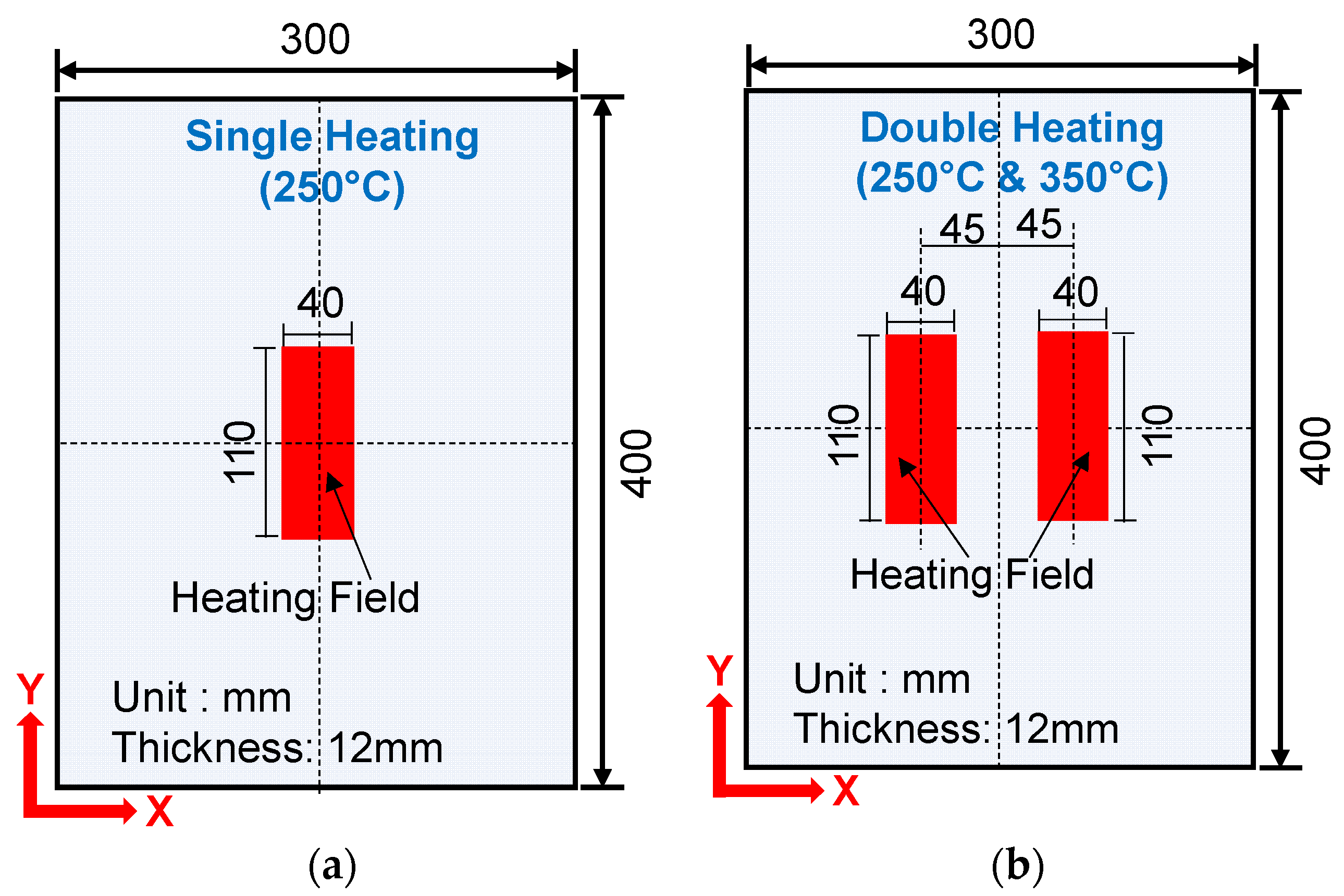
Figure 3.
Thermocouple positions: (a) Single heating and (b) Double heating.

Figure 4.
XRD measurement positions: (a) Single heating case and (b) Double heating case.

Figure 5.
Numerical models: (a) Single heating case and (b) Double heating case.

Figure 6.
Temperature-dependent material properties: (a) Physical properties; (b) Mechanical properties; and (c) Stress-strain curve.
Figure 6.
Temperature-dependent material properties: (a) Physical properties; (b) Mechanical properties; and (c) Stress-strain curve.

Figure 7.
Temperature history of Case 1: single heating (250 °C).
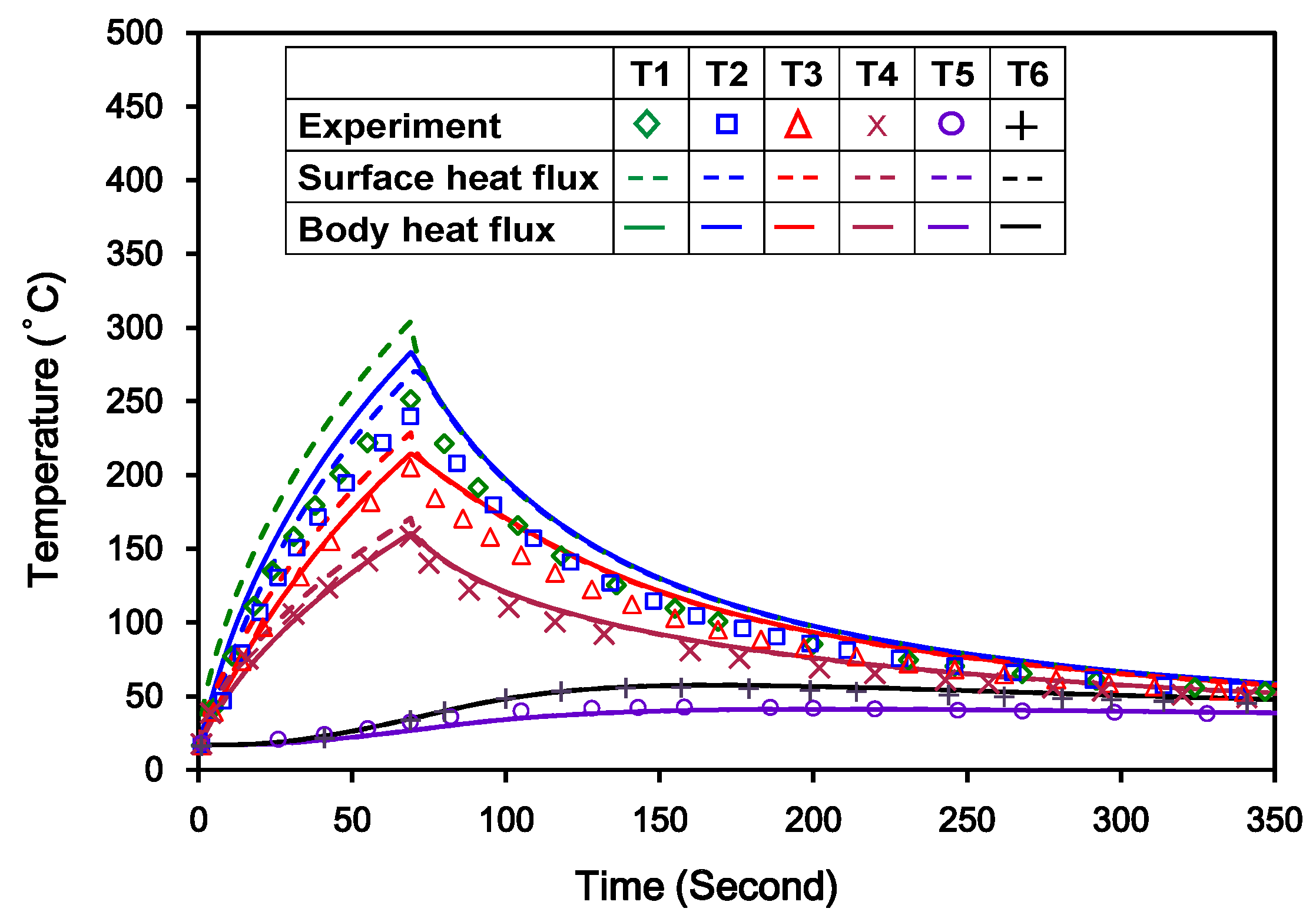
Figure 8.
Temperature history of Case 2: double heating (250 °C).
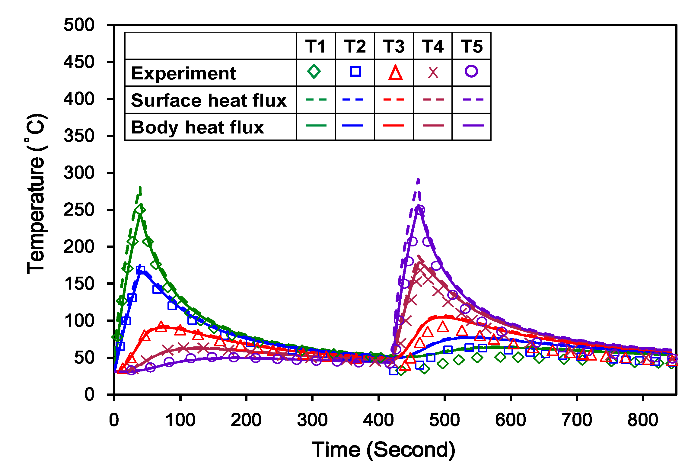
Figure 9.
Temperature history of Case 3: double heating (350 °C).

Figure 10.
Residual stresses of Case 1: single heating (250 °C). (a) Longitudinal residual stresses; (b) Transverse residual stresses.
Figure 10.
Residual stresses of Case 1: single heating (250 °C). (a) Longitudinal residual stresses; (b) Transverse residual stresses.
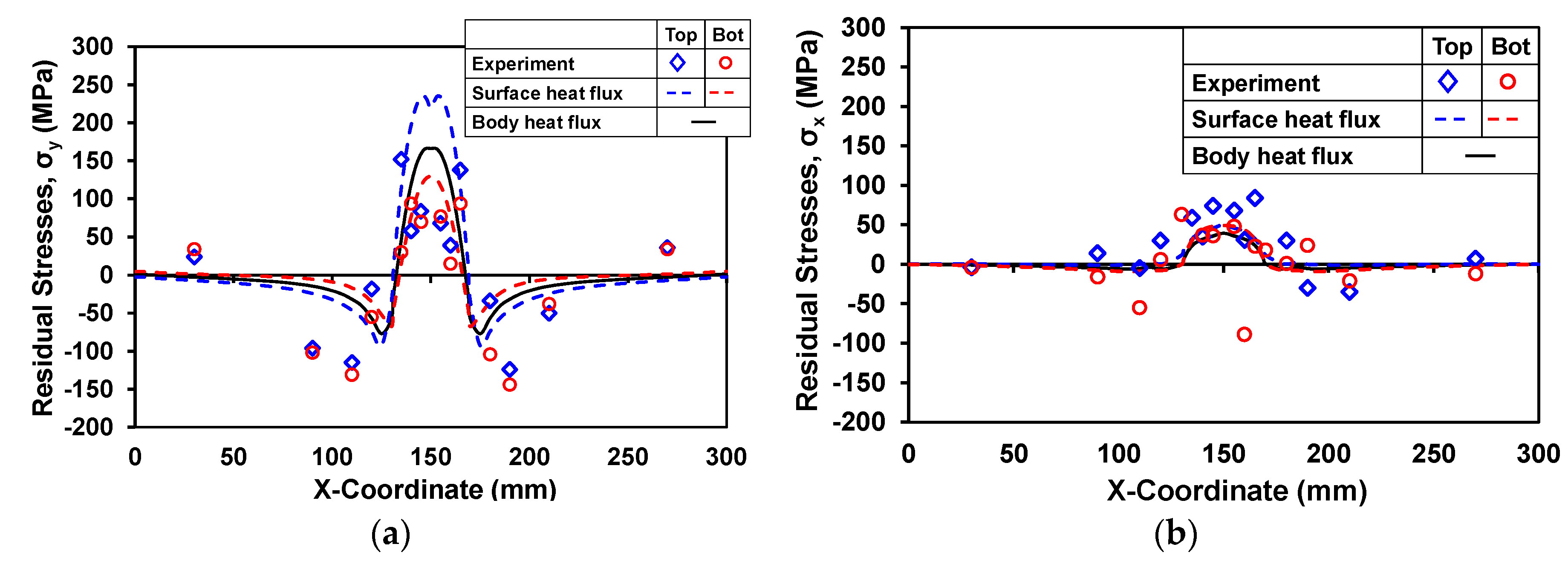
Figure 11.
Residual stresses of Case 2: double heating (250 °C). (a) Longitudinal residual stresses; (b) Transverse residual stresses.
Figure 11.
Residual stresses of Case 2: double heating (250 °C). (a) Longitudinal residual stresses; (b) Transverse residual stresses.

Figure 12.
Residual stresses of Case 3: double heating (350 °C). (a) Longitudinal residual stresses; (b) Transverse residual stresses.
Figure 12.
Residual stresses of Case 3: double heating (350 °C). (a) Longitudinal residual stresses; (b) Transverse residual stresses.


Table 1.
Chemical compositions of the base metal.
| Chemical Composition (Mass %) | ||||
|---|---|---|---|---|
| C | Si | Mn | P | S |
| 0.16 | 0.13 | 0.68 | 0.16 | 0.004 |
Table 2.
Parameters for XRD measurement.
| Method | cosα |
|---|---|
| Voltage | 30 kV |
| Current | 0.5 mA |
| Acquisition time | 45 s |
| Spot diameter | 2.0 mm |
| psi angle | 35 deg |
| X-ray diffraction peak position | 156.4 deg |
| Diffraction planes | 2.1.1 |
© 2018 by the authors. Licensee MDPI, Basel, Switzerland. This article is an open access article distributed under the terms and conditions of the Creative Commons Attribution (CC BY) license (http://creativecommons.org/licenses/by/4.0/).
Share and Cite
MDPI and ACS Style
Aung, M.P.; Nakamura, M.; Hirohata, M. Characteristics of Residual Stresses Generated by Induction Heating on Steel Plates. Metals 2018, 8, 25. https://doi.org/10.3390/met8010025
AMA Style
Aung MP, Nakamura M, Hirohata M. Characteristics of Residual Stresses Generated by Induction Heating on Steel Plates. Metals. 2018; 8(1):25. https://doi.org/10.3390/met8010025
Chicago/Turabian StyleAung, May Phyo, Masaaki Nakamura, and Mikihito Hirohata. 2018. "Characteristics of Residual Stresses Generated by Induction Heating on Steel Plates" Metals 8, no. 1: 25. https://doi.org/10.3390/met8010025
Note that from the first issue of 2016, this journal uses article numbers instead of page numbers. See further details here.