
Tactical Size Unit as Distribution in a Data Farming Environment

Finnish Defence Research Agency, P.O. Box 10, Riihimäki FI-11311, Finland
*
Author to whom correspondence should be addressed.
Axioms 2016, 5(1), 7; https://doi.org/10.3390/axioms5010007
Submission received: 19 November 2015
/
Revised: 15 January 2016
/
Accepted: 25 January 2016
/
Published: 22 February 2016
(This article belongs to the Special Issue Data Farming: Mathematical Foundations and Applications)
Abstract
:In agent based models, the agents are usually platforms (individual soldiers, tanks, helicopters, etc.), not military units. In the Sandis software, the agents can be platoon size units. As there are about 30 soldiers in a platoon, there is a need for strength distribution in simulations. The contribution of this paper is a conceptual model of the platoon level agent, the needed mathematical models and concepts, and references earlier studies of how simulations have been conducted in a data farming environment with platoon/squad size unit agents with strength distribution.
1. Introduction
Data farming improves benefits from constructive simulation. Usually agent based models are used [1], and often all units are platforms or individual soldiers as in PAXSEM by Airbus Defence and Space [2], or platforms and few soldiers as in GESI (GEfechts-SImulation System, the German word for combat simulation system) by CAE Inc. [3]. The time step in these simulations is usually one second. If we want to study large scenarios with brigade or battalion size units, use of these tools become labor intensive and computationally difficult in a data farming environment. There are two clear reasons for this. First, the time needed for the scenario building process may become prohibitively long due to the sheer number of agents. Second, the time needed for running simulations with a large number of agents may also pose a problem. An infantry battalion consists of 500–1000 soldiers and approximately 50 combat vehicles, while a brigade size unit can have over four times those numbers. Because officer training simulators like GESI [3] require tens of players, data farming with many runs becomes too slow and expensive.
Thus, there is need for larger aggregation level in large scenarios. The research questions are: given a combat situation with platoon/group size units as entities, which side wins, what is the probability of winning and what are the loss distributions for both sides. The differences in these probabilities can be used when comparing technical, tactical or logistic decision alternatives using the data farming methodology.
In this paper, we describe a platoon/group size unit as an entity in agent based simulation. This computational model of a platoon has been implemented in the Sandis simulation software [4]. There has been published papers of models used in Sandis software: the Markov model used [4] and verification of the Markov model compared with entity level calculation [5], weapon effectiveness models [4,6,7] and validation of the model in war historical context [8], but overall description of the platoon model and areal calculations inside the platoon have not been published elsewhere.
The paper is outlined as follows. In Section 2, we describe a conceptual model of platoon as entity, followed by the mathematical representation of the model, including an areal calculation model for platoon size units. In Section 3, we present validation of the simulation system and conclude in Section 4 with a discussion.
2. The Platoon as Entity in Simulation Models
2.1. Conceptual Model of an Infantry Platoon
In order to create a working computational model of a platoon size unit, a conceptual model is needed. As the basis for this conceptual model, we use Finnish forces in a forest area, as described in “The Combatant Guide” published by the Finnish Defence Forces [9].
A platoon consists of 3–4 groups/squads. The unit moves in space and time, and it has a pattern for firing at targets and actions when fired at. According to [9], a group consisting of 6–9 soldiers is scattered in an area around 100 m times 100 m depending on situation, and can shoot with light weapons up to 500–1000 m if the terrain does not restrict firing. An example of a group in line formation is shown in Figure 1. There are no exact positions of the soldiers in general, as the terrain and the mission give variations to exact positions of single soldiers. A platoon occupies a larger area, at least 300 m times 100 m.
An infantry platoon controls the area it occupies. When the platoon suffers losses, the platoon leader tries to keep control of the area by making the unit leaner until the mission becomes impossible or the company commander issues new orders. There is usually a no-man’s land between enemy and friendly platoons. Alternatively, the fight is fierce close combat, which ends with either side gaining control of the area.
A platoon size unit can concentrate its fire to the most dangerous enemy unit and can also fire effective areal fire. In the groups or squads, the leader can direct the fire with orders or by using tracer ammunition [10]. The effect of the fire depends on weapons and distance. There are test data from platoon and squad size firing [6,11].
If the soldiers in a platoon come under fire, they take cover in order to avoid casualties. According to military sociological studies [12], helping other soldiers in case of emergency is the strongest unwritten law of a military unit. When a single soldier is hit, it is reasonable to assume that his comrades pull him out of fire, give him first aid and take him to a medical facility or a medic and return to their fighting action after their wounded comrade has been taken care of. In addition, enemy fire forces soldiers to take cover, thus pinning the unit down, i.e., suppressing the unit [11]. An example of such a state machine is shown in Figure 2.
As we consider the platoon as an entity, there is no need to include each individual soldier in the model. Instead, we have the area which the individual soldiers occupy. When a unit moves, this area is moving. The firepower of a squad/platoon is similar to that of the single entity models, but the parameters are fixed to a larger unit. Losses, however, need to be modelled differently from platform level models, where a single entity unit has usually states operational or not (fully) operational, e.g., catastrophic kill, firepower kill, mobility kill, crew kill, sensor kill, and communication kill.
2.2. Computational Model
2.2.1. Markov Model for Strength Distributions
The platoon loses combat effectiveness bit by bit over time due to casualties and ammunition consumption. Thus, the strength of the unit is needed for studies. Because there are many random effects in combat, stochastic models are considered. To avoid a lot of similar simulations, a well established Markov model was selected for simulation instead of repeated single entity simulations with identical parameters (replications). This part is discussed in detail in [4], but in order to understand the whole concept, results are also repeated here.
The strength of a unit is represented by a discrete probability distribution. The unit can suffer losses during the time step. The losses range from 0% to 100%, and Figure 3 illustrates the idea of the Markov model.
When a unit is fired upon, all identical entities are expected to have the same hit probability. By denoting the unit strength distribution at time step i by J(i) and at time step i + 1 by J(i + 1), we have the matrix Equation:
where the state transition matrix T with hit probability p and q = 1 − p becomes:
This is the basic result, which can be used in calculations. The basic idea is well known Markovian modeling, see e.g., [13]. The matrix notation is from presentation by Lauri Kangas and the idea is also presented in his Master’s thesis [14]. Other formulas also exist [4]. When two platoons (Red and Blue) are in firefight, we have a probability distribution for each platoon. Let the initial strength of Red platoon be n and Blue m. In this case, we have n + 1 possible strengths for Red and m + 1 for Blue. We have (n + 1) · (m + 1) different situations in the simulation. If we assume Red and Blue distributions to be independent, we get all possible cases calculated and (n + 1) · (m + 1) new strength distributions. Computationally, the calculation is made with two loops, where Blue strength value b goes from m to zero and red value r goes from n to zero and in each case state transition matrix is created by using the combat effectiveness model. If we assume the Blue and Red distributions independent, each of these options has the probability:
The new Red and Blue distributions at the end of time step are expected values of all the cases. The assumption of independent distributions with Red and Blue units is not intuitive: if Red is winning, then Blue is losing. However, Lappi, Pakkanen and Åkesson [5] showed that the assumption of independent distributions does not lead to serious errors in calculations. This gives basic mathematics for loss calculations during the simulation, and the results are used as starting values of the state model for soldiers (Figure 3) in order to get the current strength distribution.
2.2.2. Model for Areal Distribution of the Unit
The effectiveness of weapons varies with a distance, especially with direct infantry fire like rifles and submachine guns. Artillery and mortar fire (indirect fire) with small deviation can hit effectively only a part of a unit, in which single target soldiers can be scatted over a 50,000 m2 area. In order to handle an agent with, for example, 30 single soldiers spread over a large area, some kind of inner model is needed in order to answer simulation questions like: What is the distance between target and shooter, and what are the areas where equal hit probabilities can be expected with indirect fire?
A mathematically beautiful solution would be some kind of convolution integral over the target and shooter platoon, but in that case, we have to create some kind of shooter and target density distribution. Because mathematically easy solutions such as the uniform distribution do not fit reality, a simple numerical approximation was selected. Here, the unit consists of separate calculation points, which have weighted amounts of the unit strength. These calculation points are used for distance calculations and as targets for fire.
Let us consider a numerical example of the effects of large area of an agent. Consider a platoon with three squads, nine fighters in each. The total strength is 27. Three artillery strikes hit one of the squads, e.g., the third one on the right flank of the grouping. The probability of losses is 1/3 for each strike for the unit under fire and 0 for two others. With this expectation, the average or expected value of the losses would be directly from the binomial distribution 6⅓ for the squad under fire and 0 for the two others, in total 6⅓.
Without an inner model and with only one calculation point in the center of the unit, no losses would occur, showing the need for an inner model. Consider the case where we have three calculation points each containing initially nine soldiers, i.e., the platoon strength is divided over the calculation points with equal weights. In this case, we have two basic options. First, the calculation points are used with equal number of soldiers (equal weight) for all calculation points over all future time steps, or second, separate strengths (weights) for calculation points. In the first case with equal number of soldiers (or constant weights) for each calculation point, the loss probability for single soldier would be 1/3 if being under fire and 1/3 for getting hit if under fire, ending with average hit probability 1/9 for a single target and single strike. In this case, the expected losses would be after three strikes once again from binomial distribution 8.04 instead of 6⅓. Not only losses differ but also the distribution of losses is totally different. Figure 4 shows the difference in distributions between these two calculation options.
This numerical example shows why (1) there is a need for calculation points, and (2) the unit cannot be treated as one single entity during combat simulation. Since the platoon is supposed to keep or regain the control of the area, the platoon leader will send soldiers as reinforcements to the weak parts of the positions. The calculation points are thus connected, as time passes.
Each calculation point acts as an individual entity, and soldiers fire and suffer losses independently of other points. To model a real situation, the strengths of individual calculation points are evened out over time with an exponential model, so that a calculation point that has taken heavy losses will eventually receive replacements from the other calculation points in the platoon, thus keeping the area under control with leaner strength.
We tested several calculation point formations, but, after some tests, even a simple circular formation was found accurate enough for our purposes. Figure 5 shows a unit consisting of seven calculation points spread over a circular area, with the strength of the unit divided over the points. This is a very crude estimation, but a good first version for simulation purposes, both for direct and indirect fire.
2.2.3. Model for Indirect Fire
With an aggregated unit, it is still possible to use high-fidelity weapon effect models. For computing the effects of artillery fire, a model based on the physical properties of fragmenting munitions and target elements can be used. Fragmenting munitions cause damage by high-velocity fragments, blast and heat. The impacts of individual artillery rounds on the ground can be assumed to follow a bivariate normal distribution around an aim point. The probability of a target element, representing an individual soldier or vehicle, located in a certain calculation point being killed by a single artillery round is:
where Pimpact(x, y) is the probability that the round detonates at (x, y) and Pkill|impact(x, y) is the probability that the target element is killed if a round detonates at (x, y) (see Figure 6). Pimpact(x, y) is the value of the probability density function of the bivariate normal distribution at (x, y).
The fragment effect model consists of four components: fragment zones, a fragment drag model, a fragment perforation model, and a target element model [4,7,16,17]. A fragmentation warhead is characterized by fragment zones, which are modeled as spherical zones. An illustration of fragment zones for a shell in motion is shown in Figure 7. Due to the velocity of the projectile, the angles of the zones will change and the total initial velocity of the fragments will be the resultant of the projectile velocity and the initial velocity in the static case. Fragmentation arena tests can provide experimental data on the warhead fragmentation patterns. Each fragment zone has a mass distribution and an initial velocity of the fragments. The drag model is used to compute the impact velocity of the fragments. Using the perforation equation and the fragment mass distribution, it is straightforward to compute the number of perforating fragments and further the fragment kill probability.
An accurate artillery model is good on its own but becomes almost essential when used in an aggregated model where a single calculation point represents part of a unit, not single soldiers. Traditionally, the kill probability of single artillery rounds as a function of distance from the point of detonation has been expressed by simple damage functions, instead of a physical model. The two most popular ones are the cookie-cutter and the exponent function model, illustrated in Figure 8. The circular cookie-cutter damage model with 100% losses inside a lethal radius and 0% outside is poor in general, because it does not represent the physical reality [7]. However, combined with calculation points it becomes even worse, when losses for the whole calculation point are 100% or zero.
Comparison with field tests have showed that the error of the cookie-cutter damage model is at least three times greater than that of the exponent function model and at least six times greater than the error of physical model [7]. For this reason, the physical effectiveness model is the most suitable even in an aggregated model with a platoon as agent.
2.2.4. Optimal Target Selection of Calculation Points
With the aggregated unit with several calculation points, there can be several target calculation points for each firing calculation point, as illustrated in Figure 9. Thus, an algorithm for optimal target selection for calculation points is needed. We can have a rough estimate that the soldiers want to optimize their own survival. Thus, the calculation point fires at targets which minimize the local risk to the calculation point itself. The procedure has been discussed in [15], where the optimization criterion was to minimize the risk to shooting soldiers.
The combat model calculation was used as a tool for this calculation. In the first step, the effect of fire is calculated to each target separately. The losses the target unit would cause to original shooting unit were calculated in the second step both when the unit was fired at and when it was not. This metric (difference of own losses) was used to obtain the priority of targets.
3. Testing and Validation of the Model in a Data Farming Environment
3.1. Some Simulated Cases with the Sandis Software
The original Matlab code of the model was written by Teemu Murtola in 2005. The stochastic state transition model with graphical user interface was coded using Java by Lauri Kangas and Santtu Pajukanta in 2005–2006. The Java version of the software was named Sandis in June 2006. Thus, we have almost a decade of using, testing and improving the Sandis software. Many of the simulations and test data of the Sandis simulations are classified, but there are many publications about the use of the Sandis software in different scenarios.
The calculation of platoon versus platoon situations has been published by Lappi in 2012 [4]. In Chapter 4.3.2, there is an example, which concentrates on understanding the simulated probability distribution results. In the simulation, a good shooter platoon and an average shooter platoon have firefight. The results show the winning probabilities in this case thus giving numeric utility value to the training leading to better accuracy of shooting.
Battalion or higher level combat simulation examples have been published in Sandis workshop proceedings. One case study covered a mechanized battalion repelling a tactical landing. The alternatives were fast counter attack without artillery, when the landing force has not had time to dig the positions, or to wait for artillery support, attack later. In another case study, consideration was force structure cost effectiveness, including indirect fire systems and main battle tanks. The scenario size was a mechanized battalion supported by artillery against a reinforced company supported by artillery in both cases (3rd Sandis workshop). The 6th Sandis workshop in June 2013 covered the simulation of the battle of Loimola, fought in Karelia in June 1944. In the scenario, an infantry battalion defended against four battalions. Both sides were supported by artillery. The case study is also used for validation purposes [8].
The Sandis model has been used in data farming experiments. Cases with platoon/squad size units as agents have been published in data farming workshop proceedings. In Workshop 21 in Portugal in 2010 [18] a convoy supported with mobile mortar vehicles was studied. In Workshop 29, in Riihimäki 2015, the historical battle in Loimola was studied further in a data farming setting [19].
3.2. Verification and Validation of the Model
Verification of a mathematical model usually means checking that the computer code performs the mathematical calculations correctly. Validation, on the other hand, means that the model and reality are close enough for the purpose of the model [20].
Verification of the code is easier as separate coding has been done by Laitinen [21] and Kaasinen [22]. In these studies, the state transitions and matrix calculations have been coded with consistent results with the Sandis software. In addition, separate Matlab calculations, Excel spreadsheets and Sandis software test were part of the implementation process, so the matrix calculations of the Sandis software can be considered verified.
The second question concerns validation of the model, making sure that the simulated combat results fit those of actual combat. The model is planned for comparative studies in a decision making environment, where mainly the differences between alternatives are of interest and relative goodness is enough.
The artillery model has been validated with field tests. The results of the model were within 1% accuracy of all field tests [7]. In fact, the accuracy of the physical loss calculation model is good enough for actual weapon effect calculations. The need for accuracy for comparative studies is clearly met.
The overall suitability for combat analysis has been tested with historical cases. The first attempts were made by Laitinen [13] with his own code. A full scale example using the Sandis software was conducted during the 6th Sandis workshop with simulation of the battle of Loimola. The results have been published in Tiede ja Ase 2014 [8]. In the battle, the Finnish 1st Battalion of 8th Infantry Regiment supported by heavy artillery halted the Soviet attack 26–28th July 1944. Figure 10 shows a map of the battle and a screenshot of the scenario in Sandis. The scenario size is 570 Finnish infantry soldiers and artillery and 2800 Soviet soldiers and artillery.
The Finnish data is accurate, so we can use it for comparing simulated and actual losses, which were 30 soldiers in dead and wounded. The simulated loss distribution had average of 35 with 95% interval from 25 to 44. The actual historical result is one representation of a stochastic process, so there is no significant difference between simulation and war history. The main causes for being wounded was also in good correspondence with the historical statistics. In this case, the internal model of the platoon halted the attacking Soviet units at the same positions as in the real case [8]. Thus, as the first assumption, the model seems to be valid at least for comparative studies.
4. Discussion
The Sandis software uses the platoon/group size agents instead of platform size agents. This increase in aggregation level is needed in many tactical problem solving and decision making situations in planning of the operations or acquisition optimization.
In order to have accurate models within the platoon level agents, a conceptual model is needed. The mathematical representation of the model is combination of known methods: state machines, Markov models, and physical calculation models and adaptive integration for artillery effectiveness, and predictor-corrector type optimal target selection.
The unit state model includes all possible unit strengths, thus creating calculation base for losses including a model for randomness of combat environment. Since losses affect the platoon’s ability to keep fighting, a medical action model using state machines is needed. To handle differences in weapon effects in different parts of platoon, an internal model with calculation points is needed. The calculation points created a need for optimal target selection and an accurate artillery model, which were implemented in Sandis software.
To avoid long computing, effective stochastic calculation was selected instead of Monte Carlo simulation requiring a large number of replications. The result of the simulation is directly platoon strength distribution and average values.
The Sandis and platoon model has been used in many data farming experiments and the data from a historical case fit the simulated results. The main contribution of this paper is the description of the platoon model in Section 2.1 and the description of the areal calculations inside the platoon in Section 2.2.2, which have not been published before. We conclude that a novel accurate model for comparative studies has been created, and combat simulations can be used in battalion (1000 soldiers) or brigade (4000–7000 soldiers) level simulations using data farming techniques within reasonable time and resources.
Acknowledgments
The authors would like to thank the Finnish Defence Research Agency for supporting this work and all members of the Sandis software team. Without their contribution the mathematical ideas would not be in the form of working software. The authors would also like to thank the anonymous reviewers for their comments.
Author Contributions
Esa Lappi and Bernt Åkesson wrote the paper together and have been working as a team in the Finnish Defence Forces. The original mathematical formulation of the platoon model was designed by Esa Lappi. Bernt Åkesson has been leading the Sandis software team since 2009.
Conflicts of Interest
The authors declare no conflict of interest.
References and Notes
- NATO Science and Technology Organization Modelling and Simulation Task Group 088. NATO MSG-088 Final Report—Data Farming in Support of NATO; STO Technical Report TR-MSG-088; Science and Technology Organization: Neuilly-sur-Seine Cedex, France, 2014. [Google Scholar]
- Geiger, A.; Choo, C.S.; Donnelly, T.; Erlenbruch, T.; Kallfass, D.; Schwierz, K.-P.; Wagner, G.; Seichter, S. Evaluation of Electro-optical Sensor Systems in Network Centric Operations using ABSEM 0.5. In Proceedings and Bulletin of the International Data Farming Community, Lisbon, Portugal, 19–24 September 2010; pp. 13–15.
- CAE Inc. CAE GESI™ Command & Staff Training; CAE Web Material. Available online: http://www.cae.com/uploadedfiles/content/businessunit/defence_and_security/media_centre/document/brochure.gesi.command.staff.training.pdf (accessed on 17 October 2015).
- Lappi, E. Computational Methods for Tactical Simulations. Ph.D. Thesis, National Defence University, Helsinki, Finland, 2012. [Google Scholar]
- Lappi, E.; Pakkanen, M.S.; Åkesson, B. An approximative method of simulating a duel. In Proceedings of the 2012 Winter Simulation Conference, Berlin, Germany, 9–12 December 2012.
- Lappi, E.; Pottonen, O. Combat parameter estimation in Sandis OA software. In Lanchester and Beyond—A Workshop on Operational Analysis Methodology; Hämäläinen, J.S., Ed.; Defence Forces Technical Research Centre: Riihimäki, Finland, 2006; pp. 31–38. [Google Scholar]
- Åkesson, B.M.; Lappi, E.; Pettersson, V.H.; Malmi, E.; Syrjänen, S.; Vulli, M.; Stenius, K. Validating indirect fire models with field experiments. J. Def. Model. Simul. 2013, 10, 425–434. [Google Scholar] [CrossRef]
- Lappi, E.; Urek, B.; Åkesson, B.; Arpiainen, J.; Roponen, J.; Jokinen, K.; Lappi, R. Comparing simulated results and actual battle events from 1944—A case study using Sandis software. In Tiede Ja Ase: Suomen Sotatieteellisen Seuran vuosijulkaisu n:o 72; Turunen, I., Ed.; The Finnish Society of Military Sciences: Helsinki, Finland, 2014; pp. 111–125. [Google Scholar]
- Taistelijan Opas [The Combatant Guide]. Maavoimien esikunta [Army Headquarters], Finnish Defence Forces, 2013. (In Finnish)
- Ryhmänjohtajan Opas [Squad Leaders Guide]. Pääesikunnan koulutusosasto [Defence Command Finland], Finnish Defence Forces, 1991. (In Finnish)
- Keinonen, Y. Jalkaväen Tulen Vaikutuksesta [On the Effect of Infantry Fire]; Pääesikunta [Defence Command Finland]: Helsinki, Finland, 1954. (In Finnish) [Google Scholar]
- Harinen, O. Sotilaiden Epäviralliset Ryhmänormit Kolmessa Jalkaväkikomppaniaa Koskeneessa Empiirisessä Tutkimuksessa (Knut Pipping, Roger Little, John Hockey); National Defence University: Helsinki, Finland, 2012. (In Finnish) [Google Scholar]
- Bhat, U. Elements of Applied Stochastic Models; Wiley and Sons, Inc.: Hoboken, NJ, USA, 1984. [Google Scholar]
- Kangas, L. Taistelun Stokastinen Mallinnus [Stochastic Modelling of Combat]. Master’s Thesis, Helsinki University of Technology, Espoo, Finland, 2005. [Google Scholar]
- Lappi, E.; Bruun, R.; Jokinen, K. Direct fire target selection in Sandis combat simulation. In Proceedings of the IFAC Workshop on Control Applications of Optimization, Jyväskylä, Finland, 6–8 May 2009; pp. 242–245.
- Lappi, E.; Pottonen, O.; Mäki, S.; Jokinen, K.; Saira, O.-P.; Åkesson, B.M.; Vulli, M. Simulating indirect fire—A numerical model and validation through field tests. In Proceedings of the 2nd Nordic Military Analysis Symposium, Stockholm, Sweden, 17–18 November 2008.
- Lappi, E.; Sysikaski, M.; Åkesson, B.; Yildirim, U.Z. Effects of terrain in computational methods for indirect fire. In Proceedings of the 2012 Winter Simulation Conference, Berlin, Germany, 9–12 December 2012.
- Bruun, R.S.; Hämäläinen, J.S.; Lappi, E.I.; Lesnowicz, E.J., Jr. Data farming with SANDIS Software Applied to Mortar Vehicle Support for Convoys. In Proceedings of the 21st International Data Farming Workshop, Lisbon, Portugal, 19–24 September 2010; pp. 20–21.
- Lappi, E.; Åkesson, B.; Valtonen, J.; Koskinen, J.; Hämäläinen, J.; Pentti, J.; Roponen, J.; Urek, B.; Sivertun, Å. Data Farming of a Historical Battle of Loimola in Summer 1944. In Proceedings and Bulletin of the International Data Farming Community, Riihimäki, Finland, 16–20 March 2015; pp. 18–21.
- Hartley, D.S., III. Verification & Validation In Military Simulations. In Proceedings of the Winter Simulation Conference, Atlanta, GA, USA, 7–10 December 1997.
- Laitinen, M.; Lappi, E. Can Marksmanship Explain the Results from the Kollaa Front? In Proceedings of the 2nd Nordic Military OA Symposium, Stockholm, Sweden, 17–18 November 2008.
- Lappi, E.; Kaasinen, J. Genetic optimization of tactical parameters in Sandis combat simulator. In Proceedings of the EuroGen 2007, Jyväskylä, Finland, 11–13 June 2007.
- Keinonen, Y. 1944—Taistellen Takaisin; Kustannusosakeyhtiö Tammi: Helsinki, Finland, 1971. (In Finnish) [Google Scholar]
Figure 1.
An example of a group from the Finnish Defence Forces Combatant Guide [9].
Figure 1.
An example of a group from the Finnish Defence Forces Combatant Guide [9].
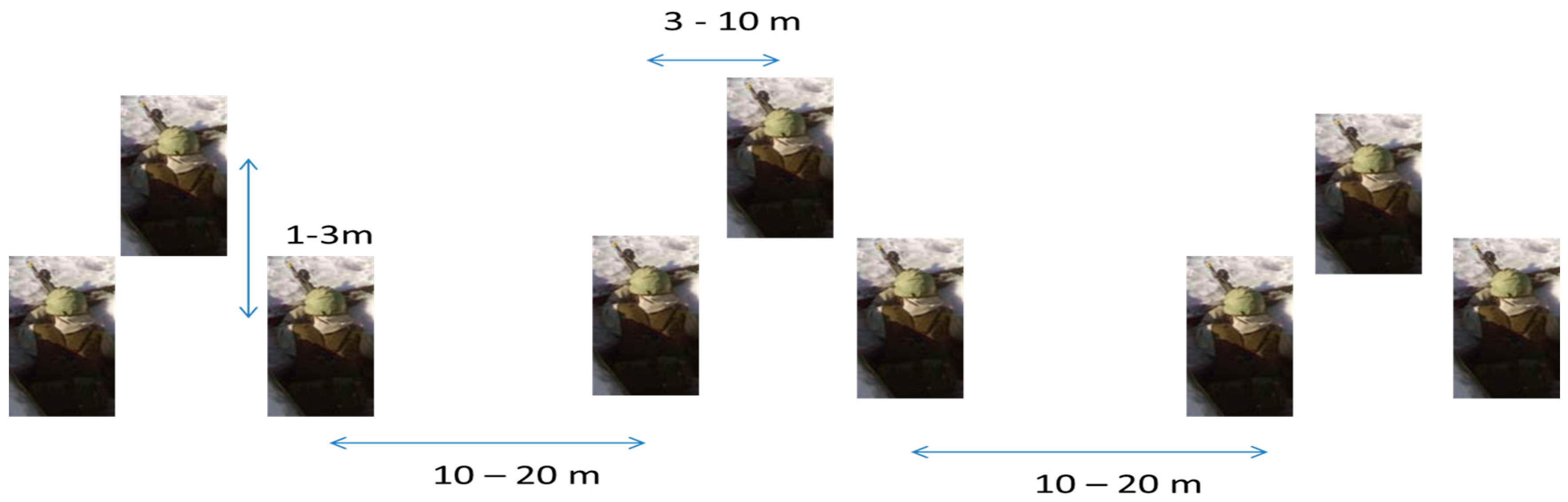
Figure 2.
A simplified state machine for soldiers at the platoon level [4], in which a soldier’s state changes over time. The unit has effective firing strength (distribution) and effective strength (distribution).
Figure 2.
A simplified state machine for soldiers at the platoon level [4], in which a soldier’s state changes over time. The unit has effective firing strength (distribution) and effective strength (distribution).

Figure 3.
The states in the Markov model represent the number of soldiers in the unit. The right hand figure illustrate the model presented in this paper, in which all transitions are in possible during each time step, except those where the unit strength would increase.
Figure 3.
The states in the Markov model represent the number of soldiers in the unit. The right hand figure illustrate the model presented in this paper, in which all transitions are in possible during each time step, except those where the unit strength would increase.

Figure 4.
The strength distributions for 27 soldiers unit after three artillery strikes when only one nine-man unit was under fire. Both expected value and deviation are different, thus illustrating the need for time-dependent inner model for platoon level agent.
Figure 4.
The strength distributions for 27 soldiers unit after three artillery strikes when only one nine-man unit was under fire. Both expected value and deviation are different, thus illustrating the need for time-dependent inner model for platoon level agent.

Figure 5.
Calculation points and weapon effect area the idea and representation from simulation software Sandis. The figure on the left is from [15] and the one on the right is from [16].

Figure 6.
The basics of artillery kill probability calculation. Reproduce with permission from [4].
Figure 6.
The basics of artillery kill probability calculation. Reproduce with permission from [4].

Figure 7.
Cross-sectional schematic of fragment zones of an exploding artillery shell. The fragment zones are modelled as spherical zones. Reproduce with permission from [17].
Figure 7.
Cross-sectional schematic of fragment zones of an exploding artillery shell. The fragment zones are modelled as spherical zones. Reproduce with permission from [17].

Figure 8.
A cookie-cutter damage model and an exponent decay model for artillery effectiveness. The exponential model is much more accurate than cookie-cutter model, but both are worse than physical model used in Sandis. Reproduce with permission from [4].
Figure 8.
A cookie-cutter damage model and an exponent decay model for artillery effectiveness. The exponential model is much more accurate than cookie-cutter model, but both are worse than physical model used in Sandis. Reproduce with permission from [4].

Figure 9.
A calculation point can shoot many target calculation points. A multi-step algorithm using weapon effect models is used to get a metric for target selection, which is used to minimize the shooters’ own casualties. Reproduce with permission from [15].
Figure 9.
A calculation point can shoot many target calculation points. A multi-step algorithm using weapon effect models is used to get a metric for target selection, which is used to minimize the shooters’ own casualties. Reproduce with permission from [15].

Figure 10.
The historical battle map by Keinonen [23] and representation in Sandis with platoon size units. The Finnish platoons are scattered over a larger area, shown by the larger circles.
Figure 10.
The historical battle map by Keinonen [23] and representation in Sandis with platoon size units. The Finnish platoons are scattered over a larger area, shown by the larger circles.

© 2016 by the authors; licensee MDPI, Basel, Switzerland. This article is an open access article distributed under the terms and conditions of the Creative Commons by Attribution (CC-BY) license (http://creativecommons.org/licenses/by/4.0/).
Share and Cite
MDPI and ACS Style
Lappi, E.; Åkesson, B. Tactical Size Unit as Distribution in a Data Farming Environment. Axioms 2016, 5, 7. https://doi.org/10.3390/axioms5010007
AMA Style
Lappi E, Åkesson B. Tactical Size Unit as Distribution in a Data Farming Environment. Axioms. 2016; 5(1):7. https://doi.org/10.3390/axioms5010007
Chicago/Turabian StyleLappi, Esa, and Bernt Åkesson. 2016. "Tactical Size Unit as Distribution in a Data Farming Environment" Axioms 5, no. 1: 7. https://doi.org/10.3390/axioms5010007
Note that from the first issue of 2016, this journal uses article numbers instead of page numbers. See further details here.