Article

Constraining the Deforestation History of Europe: Evaluation of Historical Land Use Scenarios with Pollen-Based Land Cover Reconstructions

1
Department of Archaeology, Max Planck Institute for the Science of Human History, Kahlaische Strasse 10, 07745 Jena, Germany
2
ARVE Research Sàrl, 1009 Pully, Switzerland
3
Environmental Studies Program and Institute of Arctic and Alpine Research, University of Colorado Boulder, Boulder, CO 80303, USA
4
Department of Biology and Environmental Science, Linnaeus University, 391 82 Kalmar, Sweden
5
Institute of Ecology, Tallinn University, 10120 Tallinn, Estonia
6
School of Geography, Earth and Environmental Sciences, University of Plymouth, Plymouth PL4 8AA, UK
7
Laboratoire Géographie de l’Environnement (GEODE), Centre National de la Recherche Scientifique (UMR-CNRS 5602), Université Toulouse Jean Jaurès, 31058 Toulouse, France
8
Department of Geology, Lund University, 223 62 Lund, Sweden
*
Author to whom correspondence should be addressed.
Submission received: 8 November 2017 / Revised: 14 December 2017 / Accepted: 15 December 2017 / Published: 19 December 2017
(This article belongs to the Special Issue Anthropogenic Biomes)

Abstract

:
Anthropogenic land cover change (ALCC) is the most important transformation of the Earth system that occurred in the preindustrial Holocene, with implications for carbon, water and sediment cycles, biodiversity and the provision of ecosystem services and regional and global climate. For example, anthropogenic deforestation in preindustrial Eurasia may have led to feedbacks to the climate system: both biogeophysical, regionally amplifying winter cold and summer warm temperatures, and biogeochemical, stabilizing atmospheric CO 2 concentrations and thus influencing global climate. Quantification of these effects is difficult, however, because scenarios of anthropogenic land cover change over the Holocene vary widely, with increasing disagreement back in time. Because land cover change had such widespread ramifications for the Earth system, it is essential to assess current ALCC scenarios in light of observations and provide guidance on which models are most realistic. Here, we perform a systematic evaluation of two widely-used ALCC scenarios (KK10 and HYDE3.1) in northern and part of central Europe using an independent, pollen-based reconstruction of Holocene land cover (REVEALS). Considering that ALCC in Europe primarily resulted in deforestation, we compare modeled land use with the cover of non-forest vegetation inferred from the pollen data. Though neither land cover change scenario matches the pollen-based reconstructions precisely, KK10 correlates well with REVEALS at the country scale, while HYDE systematically underestimates land use with increasing magnitude with time in the past. Discrepancies between modeled and reconstructed land use are caused by a number of factors, including assumptions of per-capita land use and socio-cultural factors that cannot be predicted on the basis of the characteristics of the physical environment, including dietary preferences, long-distance trade, the location of urban areas and social organization.

1. Introduction

The domestication of plants and animals and the establishment of agro-pastoral societies in the Holocene led to the development of anthromes, i.e., landscapes distinguished not only by their climate, topography, hydrography and natural vegetation, but also by land use [1]. Anthropogenic land cover change is one of the most important transformations of the Earth system in the late Quaternary, with biogeochemical and biogeophysical changes to the land surface that are comparable to the glacial-interglacial cycles [2]. At present, more than half of the Earth’s land surface is covered by anthromes that are dominated by human activities [3]. How, when and where this transformation of land from systems largely controlled by climate, topography and other non-human factors to those dominated by anthropogenic management occurred is important [4]. Critically, the current state of the terrestrial biosphere depends strongly on the evolution of land use systems over preceding centuries to millennia [5,6]. Anthropogenic influences on the land further led to changes in geomorphology and sediment budgets [7,8], freshwater and marine ecosystems [9] and may have influenced regional and global climate [10]. The potential of the global land base to satisfy humanity’s future demands for food, water, energy and other ecosystem services will not only be affected by ongoing climate change [11], but also by the history of land use [12] and feedbacks between land cover and the climate system [13,14].
It is therefore instructive to study the relationship between past land use and the current state of the biosphere, the role that land cover change played in the evolution of the modern climate and the perturbation of global and regional biogeochemical cycles. Observations of past land use and land cover change are, however, limited in space and time. Global monitoring of land cover based on satellite remote sensing began in about the mid-1970s [15,16]. Statistics on agricultural land use and more primitive types of remote sensing such as aerial photography extend regional estimates of anthropogenic land cover change a few decades further back in time, to the middle of the 20th century (e.g., [17,18]). National and regional-scale maps of past land use and land cover exist regionally from the late 18th century onwards (e.g., [19]). However, the terrestrial biosphere, the carbon cycle and even the global climate are influenced even today by events including deforestation and soil erosion that took place much earlier [20,21,22,23]. The importance of understanding land use history beyond recent centuries and the lack of direct, large-scale observations have led to the development of models of anthropogenic land cover change.
Because they are the only method currently available that can produce a spatially- and temporally-continuous view of past land cover change, anthropogenic land cover change (ALCC) models, and the scenarios produced by these models, are an important part of Earth system science at the present (e.g., [24,25]). ALCC scenarios have been used to estimate the impact of humans on the carbon cycle [26], regional and global climate [20,27,28], freshwater and marine ecosystems [29], geomorphology and landscape dynamics [23,30] and biodiversity [31,32], among others. Despite their utility, the evaluation of ALCC models and their scenarios has received relatively little attention [33]. ALCC models vary widely in their assumptions on the relationship between people and land use, and the resulting scenarios show enormously different timing and magnitude of past land cover change [21,33]. Conclusions drawn in research using ALCC scenarios thus depend strongly on the model that was used, and the likelihood that any individual scenario represents what actually happened in the past has been assessed only for limited periods and spatial domains. This is notably the case for the late preindustrial era in China, where globally-unique historical documents record land use change and have been successfully employed to evaluate ALCC scenarios [34,35,36].
Unlike scenarios of land use change for the future, in principle, it should be possible to determine the quality of an ALCC scenario for the past based on independent reconstructions. However, the issues described above present a problem: few independent observations have been available at appropriate spatial and temporal resolution with which to evaluate continental- and global-scale ALCC scenarios. Fortunately, recent developments in the quantitative reconstruction of land cover using paleoecological archives [37,38] and efforts to apply these methods in a synthetic way at continental scales [39,40,41] provide new opportunities for evaluating ALCC models and their scenarios.
Quantitative reconstruction of land cover using paleoecological archives, chiefly lake sediments, has its origins in palynological analysis. While the theory for the quantitative reconstruction of land cover based on pollen records has existed for decades [42,43,44,45], large-scale reconstructions only became possible more recently with the development of computer programs [37,38,46], and the intensive field studies were needed to parameterize these models regionally [39,47,48]. The REVEALSmethod of quantitative pollen-based land cover reconstruction [37], has been applied in a number of regional studies in Europe [41,46,47,49] and in sub-continental syntheses for northwestern and northern Central Europe [40,50]. This large-scale synthesis provides, for the first time, an independent estimate of land cover at a spatial and temporal scale suitable for the evaluation of ALCC scenarios.
The goals of this study were to (1) establish the relationship between quantitative pollen-based land cover reconstructions and present-day land use using land cover maps informed by satellite remote sensing that represent the modern era; and (2) with the quality of the method established, use the REVEALS reconstructions at key periods during the Holocene to evaluate two of the most widely-used ALCC scenarios: KK10 [21,22] and HYDE [51]. In the following sections, we briefly describe the REVEALS method, the KK10 and HYDE models and their scenarios, present the methodology we used to first evaluate REVEALS for the present day based on remotely-sensed land cover data and then evaluate the KK10 and HYDE reconstructions of land cover in northern and central Europe over four periods during the Holocene. A major aim of this comparison between data and models is to identify areas and periods of agreement and disagreement between the pollen-based REVEALS reconstructions and the ALCC scenarios and to provide an overall recommendation as to which ALCC model appears to be more realistic.

2. Materials and Methods

We synthesized pollen data from northwestern Europe into a land cover reconstruction and compared it to ALCC scenarios at five time windows over the middle and late Holocene. These time windows were selected to represent contrasting land use conditions at key periods during the Holocene for which it has been hypothesized that ALCC had an influence on climate [33]. The temporal range of the time windows was a function of the overall number of fossil pollen samples available in the source dataset that were included in the window [40]; the REVEALS methodology requires a large number of samples to produce a robust reconstruction [37]. The most recent window was used for calibration of the REVEALS reconstruction and covers the period from the youngest sample in each sediment core, i.e., the core top, to 100 calibrated years before present (cal. yr. bp, i.e., years before AD 1950; hereafter bp). We evaluate the ALCC scenarios for four preindustrial time windows: 6200–5700 bp (4250–3750 BC), 3200–2700 bp (1250–750 BC), 700–350 bp (AD 1250–1600) and 350–100 bp (AD 1600–1850).
To further ensure that enough fossil pollen samples were present in each time window, the REVEALS reconstructions were performed on a 1 geographic grid. We aggregated the ALCC scenarios to the same grid resolution as the REVEALS reconstructions and filtered these datasets to include only those grid cells where the pollen data were present. The driving variables, processes and output of the ALCC and REVEALS methods are summarized in Figure 1.

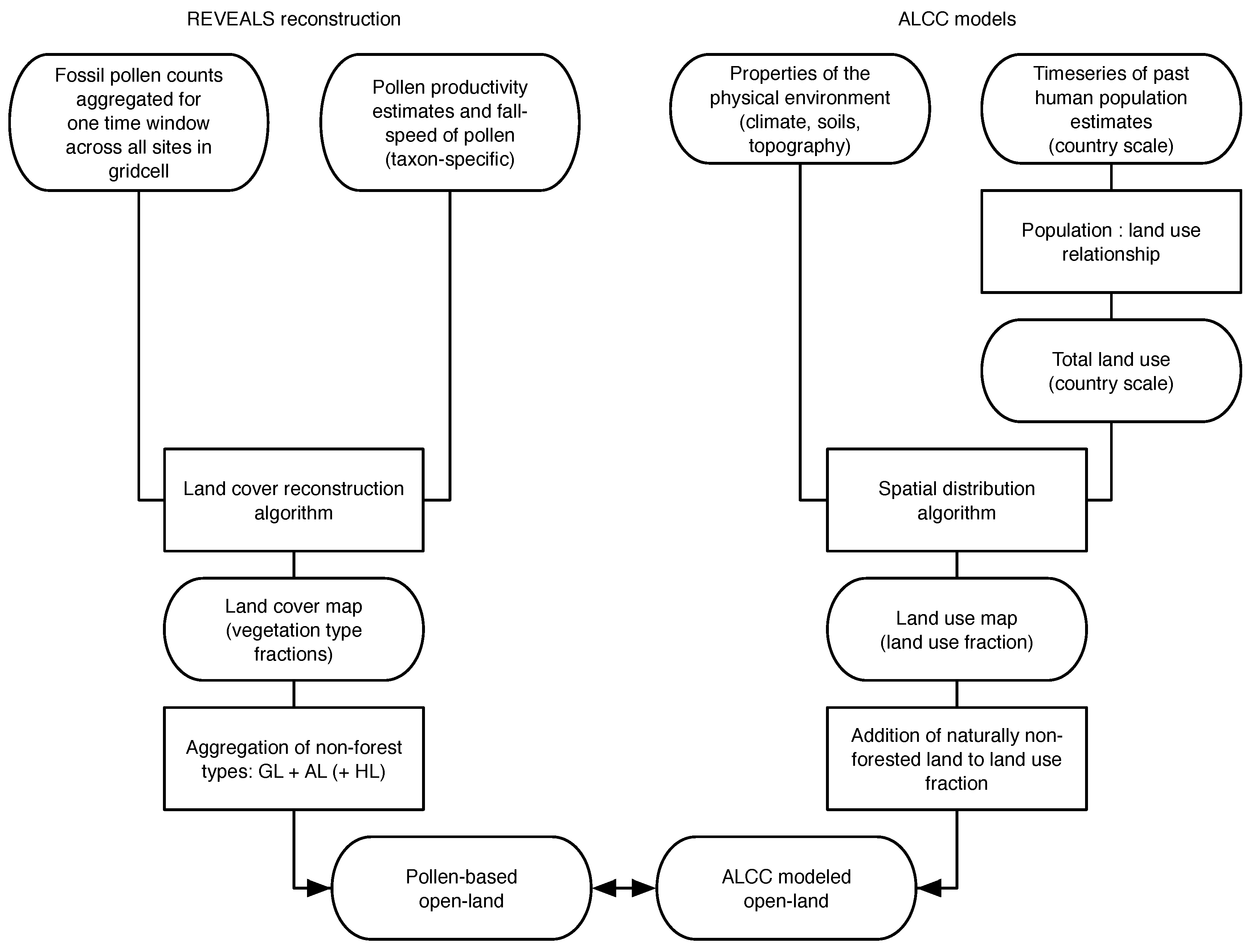
2.1. The REVEALS Pollen-Based Land Cover Reconstructions

To perform the REVEALS reconstruction, we aggregated pollen counts from all samples in a corresponding time window for each pollen record. Samples came from sediments collected in lakes of a range of sizes and from peatlands; see [40] for details on the selection of the pollen records. The number of pollen records available for the reconstruction varied depending on the 1 grid and time window. The REVEALS program estimates the mean regional vegetation composition of each of 25 taxa with its standard error in each grid cell for each time window whenever data are available. Pollen productivity estimates (PPEs) and fall speeds of pollen (FSP) used in the REVEALS runs are found in [47]. The grid-based REVEALS taxon estimates are then classified and converted to the estimates for 10 plant functional types (PFTs), hereafter referred to as the “grid-based” REVEALS PFT estimate (GB REVEALS PFT). The full protocol of the LANDCLIMREVEALS runs is found in [40].
While REVEALS provides the estimates in the coverage of each of 25 taxa on the landscape, the ALCC scenarios contain only a single quantity defined as “land use”. In the northern and central European context for the mid to late Holocene, land use generally implies deforestation, or the conversion of forest and shrubland to arable land and pasture. We therefore aggregated the REVEALS land cover fractions into an estimate of land use that we expected to be comparable to the ALCC scenarios.
Because the potential natural vegetation of the vast majority of our study area is forest [52], we define used land in the REVEALS reconstructions as the non-woody fraction of the landscape. This includes the GB REVEALS PFTs “agricultural land” (AL) and “grassland” (GL) [40,47], which were summed to produce an openness fraction. AL includes the REVEALS estimates of cover for all cereals, and GL includes the REVEALS estimates for eight taxa together: Artemisia, Cyperaceae, Filipendula, Poaceae, Plantago lanceolata, P. media, Littorella-type and Rumex acetosa-type [33,40]. In Europe, heathlands may be considered either anthropogenic or natural [53,54]. For this reason, we further performed a set of comparisons with REVEALS that include heather (Calluna vulgaris, hereafter “heathland” or HL) in the open fraction.
Other types of naturally open land, e.g., natural meadows and peatlands, are not explicitly considered in our study. Peatland may have been both created, e.g., in Scotland and Ireland [55], and destroyed, e.g., in The Netherlands [56], as a result of land use during the preindustrial era. These sorts of land use changes might be difficult to detect in the pollen record and are not considered in the ALCC scenarios.
The REVEALS reconstructions are provided with an uncertainty estimate for each grid cell and time window. Standard errors of the mean plant composition among sites in each grid (GB REVEALS taxon estimate) are estimated using a hybrid of the delta method and Monte Carlo simulations [37,38]. In this calculation, the error estimates on the pollen productivity estimates are also taken into account. The standard errors of each GB REVEALS PFT, here AL, GL and HL, and of the GB REVEALS PFT AL + GL and AL + GL + HL are also calculated using the delta method [40,47]. See Appendix A for a further discussion of the sources of uncertainty in the REVEALS method.

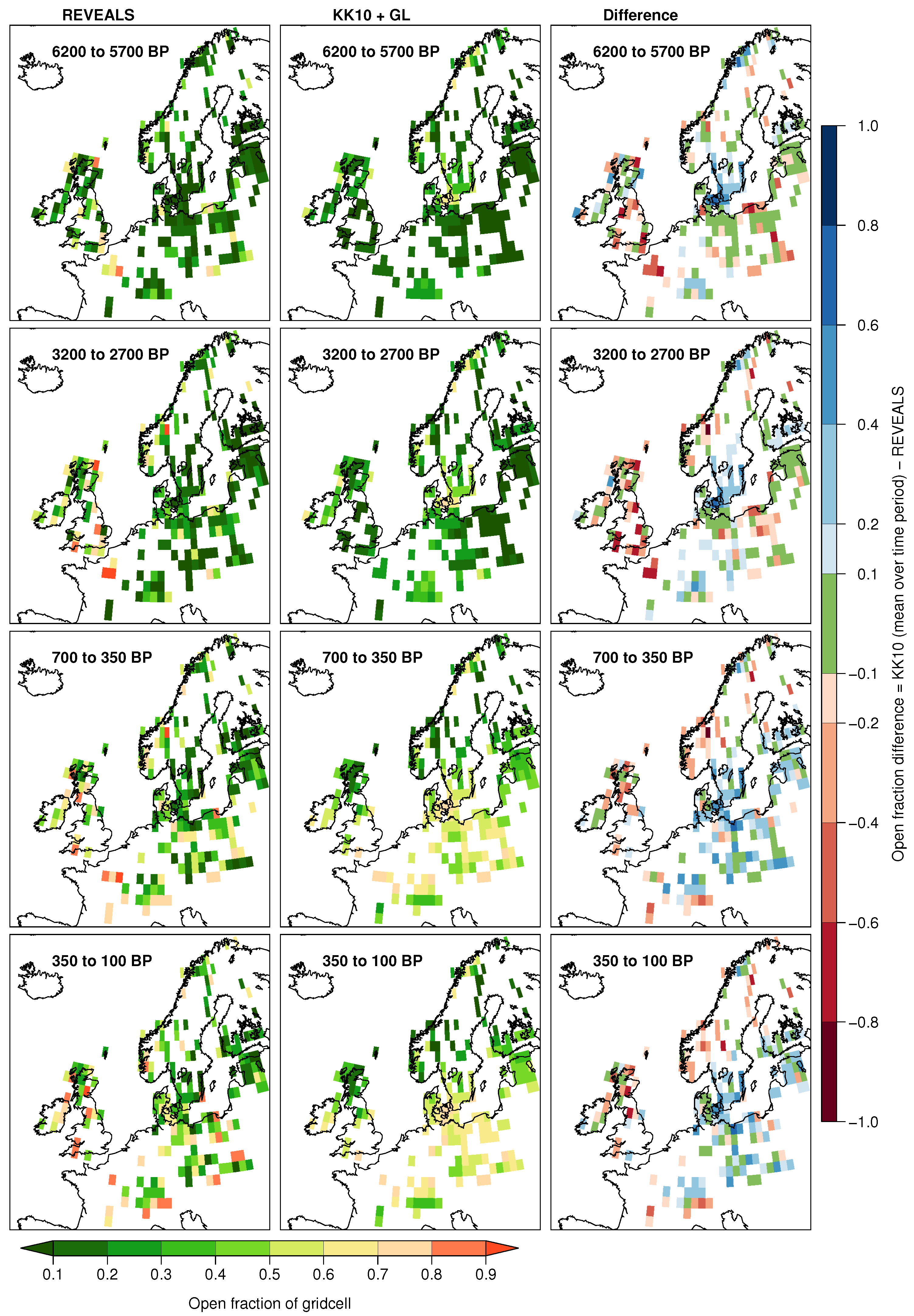
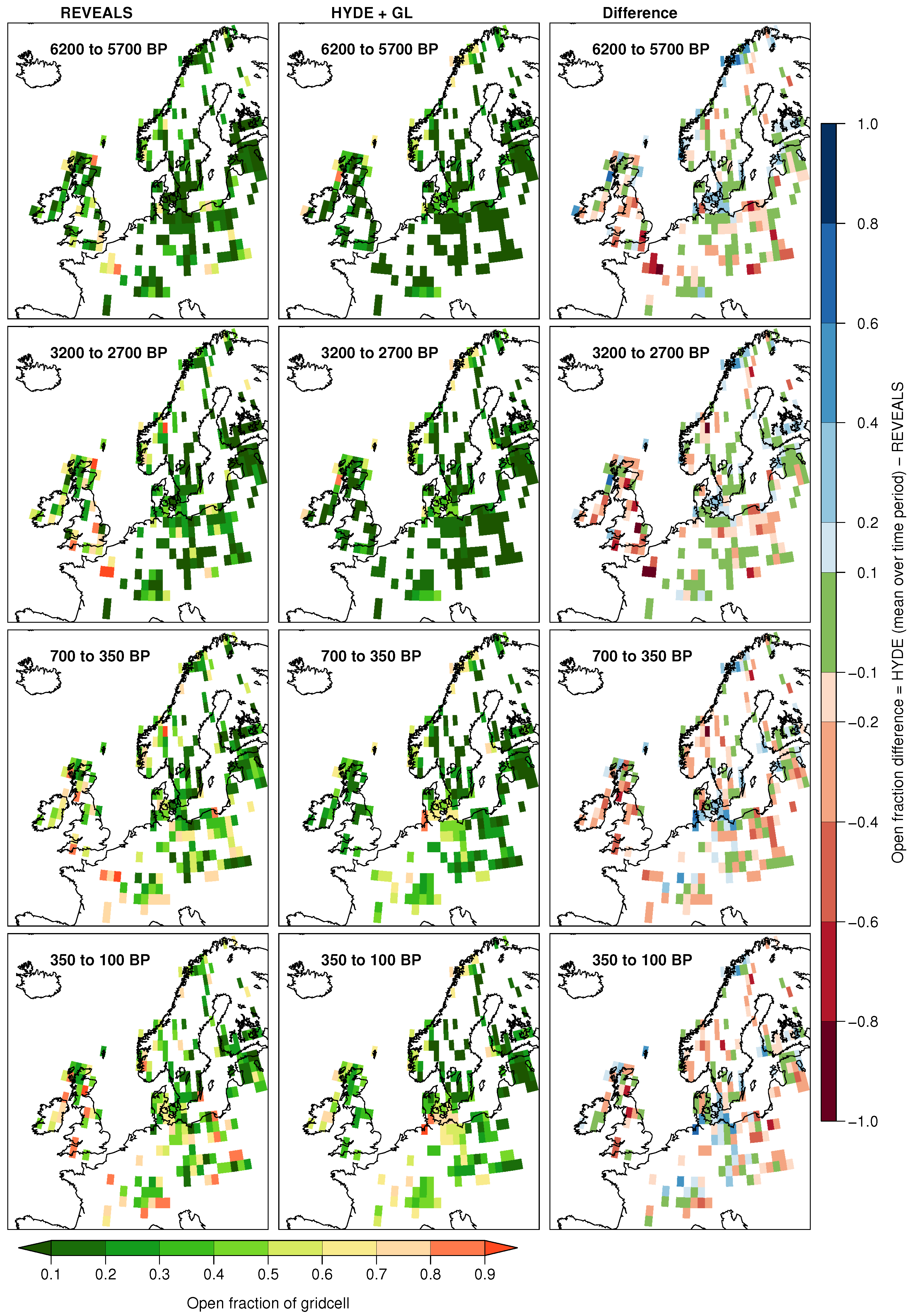
2.2. The KK10 and HYDE ALCC Scenarios

KK10 and HYDE are GIS-based models that translate information on human population, suitability for cultivation and pasture based on the properties of the physical environment and other physiographic factors, e.g., distance to coastlines or rivers, into scenarios of anthropogenic land cover change [22,51]. Both models make the major assumption that the properties of the physical environment are stable over time, i.e., they do not explicitly account for the effects of Holocene climate or geomorphic change or variability influencing suitability for land use. On the other hand, both models are driven by spatially explicit, temporally-varying estimates of past human population. In both KK10 and HYDE, these are provided at approximately the country level, with some larger countries divided into subregions, e.g., oblasts in Russia [6]. For Europe, population estimates used in both KK10 and HYDE are based primarily on demographers’ estimates for the last 3000 years [57], with increasing uncertainty back in time. For periods earlier in the Holocene, HYDE uses back extrapolation while KK10 is driven by a model of potential population [21,58]. Total land use at the regional level is estimated as a function of population and then distributed in space as a function of the physical environment.
The principle difference between KK10 and HYDE is the relationship between total population and land use. HYDE assigns a nearly constant value for per-capita land use for the entire period prior to AD 1961, the first year for which harmonized global statistics for land use are available [51]. KK10, in contrast, uses a logistic function relating land use to population density on usable land, which results in much larger amounts of per capita land use with lower densities [22]. In HYDE, per capita land use is between 0.5 and 1 ha per person for nearly all of the prehistoric and preindustrial era, while for KK10 per capita land use varies from 8 ha per person to less than 1 ha per person, depending on region and time (see Figure 2 in [21]).
With this basic model structure, both KK10 and HYDE are capable of creating a number of ALCC scenarios that account for uncertainties in the underlying driver data and even the form of the relationship between population and land use. For the comparison with REVEALS, we assigned an uncertainty range to both KK10 and HYDE ALCC estimates at each of the periods’ studies. For KK10, we aggregated the results of six individual runs from the model in order to estimate uncertainty in the scenarios. The individual runs were developed by running the model with a range of population estimates: “best guess”, upper, and lower bounds and two different relationships between population and land use. In the standard relationship, the logistic curve is the same at all periods, while in the technology simulations, the shape of the curve changes over time, with increasing per capita land use at the same population density further back in time. Both scenarios are described in detail in [22]. In this study, we assign the ALCC estimate as the mean of the six KK10 scenarios, with error bars representing the range of values present across all scenarios. For HYDE, only a single scenario was available at the time we performed the analysis, so we used the published estimates of model uncertainty to provide an error range in the comparison with the REVEALS reconstructions. Uncertainty in HYDE is estimated at 5% in AD 2000, 50% at 1950 bp and 75% at 11,950 bp [51]. For each comparison period, we assign HYDE an uncertainty range by linearly interpolating the error estimate at these dates to the mean year of the comparison period.
KK10 covers the period 8 ka–AD 1850, and HYDE 3.1 extends from 10 ka–AD 2000. In the HYDE scenario, the amount and spatial distribution of land use in the second half of the 20th century are based on satellite remote sensing combined with FAO land use statistics. These independent observations of land cover make the present-day land use maps in HYDE a reasonable starting point for the evaluation of the quality of the REVEALS open land estimates.

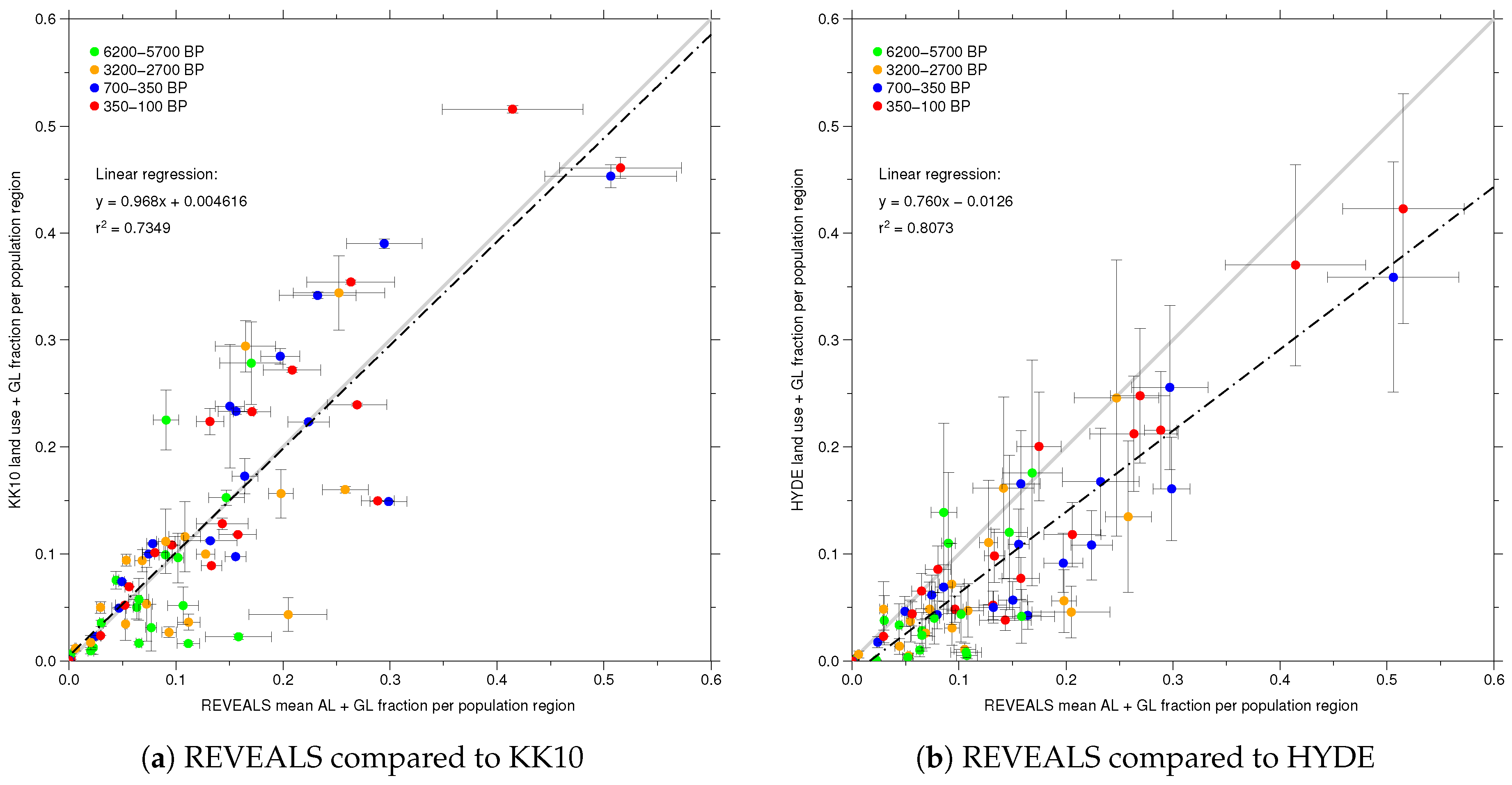
2.3. Comparison between REVEALS and the ALCC Scenarios

To perform an evaluation of the quality of the REVEALS method, we compared the first REVEALS time window (0–100 bp) with the mean of the HYDE scenario over the same period. The original KK10 scenario extends to AD 1850, and for studies covering the most recent period, it has been merged with HYDE [5], so KK10 was not used in the evaluation of the modern time window. For the four periods covering the rest of the late Holocene, we compared both the KK10 and HYDE datasets with the REVEALS reconstructions.
Comparison of the ALCC scenarios with the REVEALS reconstructions required a transformation of the spatial and temporal resolution of the ALCC model output. While the ALCC scenarios were available at 5 arc-minute resolution, the REVEALS reconstructions were prepared for 1 grid cells where sufficient pollen data were available. For comparison between the ALCC scenarios and REVEALS, we aggregated KK10 and HYDE to the REVEALS grid by averaging the land use fraction in each block of 12 × 12 (144) 5-min grid cells. We performed the comparison only on grid cells that contain REVEALS reconstructions, i.e., all grid cells from the KK10 and HYDE that did not have a corresponding REVEALS estimate were masked out of the following analyses.
KK10 was produced at annual resolution and was therefore averaged over all of the years in each of the four time windows in this study to obtain estimates comparable with REVEALS. HYDE contains ALCC estimates at irregularly-spaced time windows over the Holocene: 1000-year intervals prior to 2 ka, 100-year intervals from 2 ka–AD 1700 and decadal intervals to the present. For comparison with the REVEALS time windows, we linearly interpolated land use fraction in the HYDE scenario between the years for which it was produced and averaged these over the years of the time window.
For comparison between REVEALS and KK10 and REVEALS and HYDE, we assumed that land use in the ALCC scenarios should be roughly equivalent to the open land (non-forest) fractions in REVEALS. We defined open land in REVEALS as the sum of the AL and GL fractions and performed a supplementary set of comparisons where we further added heather (HL) to the open land fraction. This assumption is of course not valid in areas that are naturally non-forest, e.g., in high mountains and at high latitudes. In order to make the ALCC scenarios comparable to REVEALS reconstructions, we added the naturally non-forested areas identified in [22,59] to the land use fraction in the ALCC scenarios. This addition of naturally open land areas to the KK10 and HYDE resulted in increased open land mainly in the far north of the Nordic countries and in high mountain areas, but did not result in large changes for most of the naturally forested populated areas of northern and central Europe.
A preliminary analysis comparing openness fractions on a grid cell-by-grid cell basis showed very little correlation with either the KK10 or the HYDE dataset (Figure S1). We therefore elected to compare openness fractions on the spatial unit of roughly country-sized population regions. These population regions represent the smallest spatial unit covered by a time series of population data [22] that were used to drive the ALCC models. For each time window and for grid cells where REVEALS data were available, the area of open land within each population region was summed and divided by the total area of the region. In this manner, we evaluate the quantity of modeled land use within approximate geographic regions, but not necessarily its distribution on a grid-cell by grid-cell basis.
To quantify the relationship between REVEALS and the ALCC scenarios, we fitted linear regressions [60] between the REVEALS mean open land fractions per population region and the open land fraction for each modeled ALCC scenario. An identical series of regressions was performed for REVEALS open land fractions that included heather (Figures S2–S5).

3. Results

In Figure 2, we present the relationship between REVEALS and HYDE for the modern era (0–100 bp). For this period, land use in Europe in the HYDE scenario is largely based on remotely-sensed land cover and therefore reflects the “real” distribution of open land at a time close to the present. While the spatial distribution of non-forested land does not match precisely between the HYDE and the REVEALS reconstructions (Figure 2, maps; see also Figure S2 for results that include heather as part of the open fraction), the open fractions between the two datasets correlate very well (slope of the regression line 0.971; r 2 = 0.925) when aggregated into country-sized population regions (Figure 2, lower right plot). For comparisons that include HL as part of the open fraction in REVEALS, the correlation is not as good (slope: 0.828), indicating that REVEALS reconstructions that include HL are consistently higher than HYDE open fractions.
In Figure 3 and Figure 4 (and Figure S3 with HL), we present spatial comparisons between the REVEALS reconstructions and each ALCC scenario (KK10 and HYDE) at the four preindustrial-Holocene time windows. Both maps of openness fractions and difference maps are shown. In the earliest time window, 6200–5700 bp (4250–3750 BC), the REVEALS reconstruction depicts a completely treeless landscape in only two grid cells: one in northern Scotland and the other in northern France. In several other areas, such as in Poland and along the English Channel, semi-open landscapes are reconstructed. For this period, KK10 suggests that nearly all of the study area was forested, with only some grid cells showing semi-open vegetation in southern Sweden and western Ireland (Figure 3). Europe during this time period was also forested according to HYDE, except for one grid cell in western Scotland that is 80% open (Figure 4). When the REVEALS reconstructions of non-forest land are subtracted from the ALCC scenarios (difference map), the HYDE and KK10 openness fraction matches the REVEALS estimates well (±10%) in many grid cells.
During the second time window (3200–2700 bp; 1250–750 BC), there is an increase in the open fraction of the landscape in the REVEALS reconstruction in northwestern Europe. Grid cells with 80% openness or more can be found in Norway, Scotland, southern England and the Normandy region of France. The ALCC scenarios do not show deforestation in these exact areas. KK10 shows only slightly more landscape openness than in the previous period and with the same spatial distribution, mainly in southern Sweden and western Britain and Ireland (Figure 3). The HYDE reconstruction shows a nearly identical landscape to the previous time period (Figure 4). Both ALCC models severely underestimate the openness fraction in Britain and in northern Poland compared to the REVEALS reconstruction.
In the 700–350 bp (AD 1250–1600) time window, the REVEALS reconstruction shows a heterogeneous opening of the landscape throughout central Europe, with many grid cells having 70–80% open land. KK10 shows about 40–80% deforested land in central Europe, but landscape openness is distributed more uniformly across the landscape than in the REVEALS reconstructions, resulting in an overestimation of the openness fraction in many areas (Figure 3). HYDE shows somewhat more open land during this period relative to the earlier time windows, primarily in northern Germany along the North Sea and in the northeast of France, near Luxembourg (Figure 4). In contrast to the earlier periods, the REVEALS reconstruction shows a large degree of open land in the Alpine region at this time, with many grid cells reconstructed as more than 70% open land. Neither KK10 nor HYDE capture this opening of the landscape; the Alps are largely forested during this period in both scenarios. Both ALCC models show spotty agreement with REVEALS in central Europe, but underestimate the amount of open land in Norway. We still observe lower fractions of openness in Britain in the ALCC scenarios when compared to REVEALS. KK10 however shows good agreement with REVEALS at grid cells in Ireland and Denmark, and HYDE has good correspondence to REVEALS in southern Poland and in areas bordering the Baltic Sea. In general, KK10 has more grid cells depicting slightly greater amounts of open land than REVEALS, while HYDE generally has smaller amounts of open land compared to the pollen-based reconstructions.
The final preindustrial time window at 350–100 bp (AD 1600–1850), shows further clearance (90% or more) in REVEALS in the same grid cells that were partially deforested in the previous period, chiefly in Britain, the Alps and in some areas of Poland and the Czech Republic. In central Europe, KK10 agrees with REVEALS with roughly 60–70% deforested fraction. In contrast, KK10 does not capture the magnitude of landscape openness reconstructed by REVEALS in Britain. The difference map between REVEALS and KK10 looks similar to the difference map from the previous time window. HYDE shows patchy areas of open land, but the magnitude of landscape openness is substantially lower than the REVEALS reconstruction and not always in the same places, e.g., in northern Germany.
Overall, the ALCC scenarios do not compare well with the REVEALS reconstructions at grid cell-by-grid cell level (Figure 3 and Figure 4; see also Figures S1 and S3). KK10 tends to be in better agreement with REVEALS in areas where REVEALS depicts open land, while HYDE matches REVEALS better in areas where there is less open land in REVEALS. HYDE generally underestimates landscape openness with respect to REVEALS, while KK10 overestimates landscape openness, especially during the latter two time periods. When heather is included as part of the REVEALS open fraction (HL maps, Figure S3) some areas, Britain and Denmark in particular, appear much more open at all periods analyzed.

3.1. Comparison at Population Region Scale

In Figure 5, we present aggregate correlations between open land area in country-sized population regions for the REVEALS reconstruction relative to the ALCC scenarios. Each data point on these plots represents open land fractions for a single population region and time window. Data points above and below the 1:1 line indicate that the ALCC models simulate larger and smaller open areas than the REVEALS estimates, respectively.
Figure 5a displays the correlation between REVEALS and KK10 openness fractions. A linear regression of the data results in a slope of 0.968 with a y-intercept close to zero, indicating that a strong correlation on a population region-scale exists between KK10 and REVEALS. In the earlier periods (6200–5700 bp and 3200–2700 bp), REVEALS shows slightly higher estimates of open land than KK10 (cluster of orange and green points at the lower left corner of the plot). In contrast, the later two time windows fall above or around the 1:1 line. The r 2 value of 0.735 indicates that there is some scatter, but overall, the correlation is fairly good. When HL is included as part of the REVEALS openness fraction, the correlation with KK10 is not as strong, with a slope of 0.666 and a lower r 2 of 0.592 (Figure S4, left panel).
The REVEALS-HYDE correlation at the population region scale (Figure 5b) shows that HYDE consistently underestimates open land with respect to REVEALS. A linear regression through the data results in a slope of 0.760. A majority of the data points fall below the 1:1 line, indicating that even when data are aggregated into population regions, HYDE has less open land than the REVEALS reconstructions during preindustrial times. This trend is further emphasized if heather is included in the REVEALS open fraction estimates, shifting the REVEALS estimates even further to the right (Figure S4, right panel). In this case, the slope falls to 0.544, well below the 1:1 line.

3.2. European Totals: An Overview of the Preindustrial Intercomparison

The increase in percentage of open land through time within our study area, i.e., the grid cells covered by REVEALS reconstructions, simulated by the KK10 and HYDE models and reconstructed with REVEALS is presented in Figure 6. This overview further demonstrates that, on a European scale, the HYDE open land estimates are roughly 25% smaller than REVEALS during preindustrial time. However, the wide error range of HYDE encompasses the REVEALS estimates in all but one period (700–350 bp). The KK10 land use estimates are lower than those of REVEALS during the first two time periods, but are within the error range. During the two last time windows, the KK10 scenario overestimates open land relative to REVEALS. Including heather (HL) in the REVEALS estimates increases openness in Europe, especially during the first three REVEALS time periods (Figure S5).

4. Discussion

Comparison of REVEALS with land use observations largely informed by satellite remote sensing for the “present-day” time window (0–100 bp) shows that the REVEALS estimates of open land fractions are realistic in magnitude and spatial distribution. The REVEALS estimate of open land for this period is largely controlled by the core-top or youngest sample in the record, which in practice integrates over a 10–50-year period depending on the sedimentation rate, dating up to and including the year when the site was collected (ca. AD 1970–2010). The HYDE land use data used as a comparison is largely a function of present-day land cover observed with satellite remote sensing, combined with national land-use statistics on crop and pasture. During this period, major cities and agricultural areas were in roughly the same location as at present. As the uncertainty in HYDE for this period is low (ca. 11%), the fact that REVEALS and HYDE have good correspondence (Figure 2) is evidence that the REVEALS algorithm works reasonably well for translating pollen percentages into land cover, as has been demonstrated earlier for several sub-regions of Europe [46,61,62]. Comparisons of HYDE with REVEALS reconstructions that include the heather (HL) fractions do not match as well (slope of 0.828; Figure S2), and we omitted HL from our primary analysis. Though heathlands can develop due to anthropogenic influences such as grazing and fire, many are natural and do not result from human activities [53,54,63]. This evaluation of the REVEALS method provides confidence that the REVEALS reconstructions are suitable for the evaluation of KK10 and HYDE scenarios for preindustrial time.
For the preindustrial Holocene periods we examined, a distinguishing feature of the REVEALS reconstructions for northern and central Europe is that landscape openness was high in some relatively confined areas in Europe. Open areas expanded gradually with time, but landscape openness in Europe remained heterogeneous, expanding out from previously-cleared settlements, while closed forests persisted in certain areas. In contrast, forest opening in the KK10 dataset is quite diffuse, especially in areas with relatively homogenous suitability for agriculture, such as the lowlands of France and Germany. In HYDE, landscape openness is patchier, but tends not to be in the same areas as those reconstructed by REVEALS.
In fact, it is very difficult to see any correspondence between the ALCC scenarios and the spatial pattern of landscape openness reconstructed by REVEALS at the level of individual 1 grid cells (Figure 2, Figure 3 and Figure 4), an observation that is further highlighted when directly comparing corresponding grid cells (Figure S1). One of the main areas of mismatch is in Britain, where both KK10 and HYDE models consistently underestimate land use when compared to REVEALS, which shows substantial fractions of open land in northern and western Britain (Figure 3 and Figure 4, difference maps). The open land fractions in REVEALS are even greater when including heather (Figure S2). Land suitability for cultivation is low in these regions due to the cooler climate and poor soils, resulting in land use and thus landscape openness concentrated in southeastern England in both KK10 and HYDE [22]. Neither HYDE nor KK10 explicitly quantify land that has been deforested as a result of deforestation for construction or fuel wood, nor do they attempt to model certain types of extensive land use such as the creation and management of anthropogenic moorland pasture, a preindustrial anthrome that was particularly common in Britain [64,65] and parts of Denmark [66]. This mismatch in Britain highlights the need for models to cover a broader range of human influence on vegetation, rather than just deforestation for agriculture. This may also be one of the reasons for the underestimation of landscape openness in western Norway (see Figure 3 and Figure 4, red areas on difference maps); however, disagreement could also be due to an underestimation of the area of naturally non-forested areas [59] or an issue with representing this ecological setting from pollen data in the REVEALS reconstruction.
The Alpine region is also an area of important disagreement between REVEALS and the ALCC scenarios, particularly during the 700–350 bp and 350–100 bp time windows. REVEALS estimates that these mountainous areas were 70–90% open land during these last two preindustrial periods. Land is deemed as being too cold for agriculture using the KK10 methodology, even though transhumant pastoralism has been common in these areas since at least the Bronze Age [67]. HYDE did not distribute land use in the Alpine region likely for the same reasons as in KK10 and also because HYDE concentrates land use in areas with low slope. However, severe deforestation is documented to have occurred in the Alps in the late preindustrial era (e.g., [68,69]). Crises such as floods and erosion occurring just prior to industrialization in France and Switzerland prompted legislation protecting montane forests and encouraging reforestation in the late 19th century [68,70]. The REVEALS reconstruction shows an increase in the forested area of the Alpine region between the 350–100 bp and 100–0 bp time windows (Figure 2 and Figure 3). However, making historical inferences from the REVEALS reconstruction can be problematic due to both the low sampling resolution in many of the source pollen records, particularly near the core top, and the large time windows used here. For instance, REVEALS shows that Ireland was roughly 40% (on average) forested during the 350–100 bp time window, while historical sources state that Ireland has been covered by less than 5% forest since the beginning of the 17th century [71].
The fact that the correlation between REVEALS and KK10 and HYDE is poor when making comparisons on a grid cell-by-grid cell basis may lead us to conclude that the ALCC models are incapable of reconstructing the spatial pattern of past land use. However, the models do better when compared to the pollen-based reconstructions on broad geographical regions, such as the population regions used in this study. Indeed, the KK10 data come close to a 1:1 correlation with REVEALS when comparing the amount of open land in each population region (Figure 5a). This lends support to the validity of the relationship between population density and forest cover that is behind the KK10 model [22], at least for northern and central Europe. On the scale of Europe as a whole, KK10 tends to slightly underestimate landscape openness during the earliest two time windows while it overestimates landscape openness during the latter two periods (Figure 6). Though the REVEALS reconstructions display a sigmoidal increase in open land with time, it appears to increase more gradually as compared to KK10 (Figure 6). The sigmoidal relationship that KK10 uses to translate population density to land use was developed based on historical data for France, Ireland, Denmark and Sweden, all areas partially covered by the REVEALS data, but is likely to be not representative of all of Europe. Another reason for the more gradual increase in open land could be due to the broad time windows used in the REVEALS reconstructions. HYDE, on the other hand, shows an even more gradual, near linear relationship between open land and time and tends to underestimate preindustrial land use with increasing magnitude towards the present (Figure 6).
The linear regression between REVEALS and HYDE shown in Figure 5b has a slope of less than one, indicating that HYDE consistently underestimates land use as compared to REVEALS. Total open land in the entire study area is also low for each preindustrial time slice (Figure 6). A major reason for the lack of landscape openness during the preindustrial period in the HYDE database is the use of late 20th century (AD 1961) values for per capita land use that are nearly constant throughout the entire dataset. Mechanized agriculture, high yielding crop varieties, fertilizers and pesticides all contributed to a significant decrease in per capita land use during the mid-20th century. Over the past 7 ka, technological and socio-cultural developments could have led to roughly a 10-fold decrease in per capita land use [21,72,73]. We suggest this as the main reason why the HYDE scenario for the preindustrial period is smaller than those in the REVEALS reconstruction.
While the magnitudes of used or open land estimates are more similar between KK10 and REVEALS, both ALCC models need improvement on the distribution of land use in the past. In fact, distributing land use based on a large-scale gridded climate and soil datasets offers only a rough estimate of places that would have been hospitable to preindustrial farmers and pastoralists. While agriculturalists usually favored fertile loess soils and areas where natural vegetation could be cleared and soils prepared using fire and with the tools of the era [74], there are other factors that influence the selection of a settlement location, e.g., position along trade routes, distance from non-agricultural food resources, defense and other strategic reasons that are not easily predicted on the basis of the properties of the physical environment. The compilation of archaeological 14C dates can be used to infer settlement patterns in the distant past (e.g., [75,76,77,78]), and it could be possible to interpret this information as a proxy for land use. Incorporating geographical data on diet, social organization, settlement density and other socio-cultural characteristics would also aid in achieving a more accurate distribution of past land use since urbanization [79,80]. Closer in time to the present day, land use and human settlements in the more recent past are easier to distribute in part because landscapes in Europe become “fully occupied”, i.e., nearly all of the usable land in a region is under some sort of human influence, and because there is less uncertainty in the population estimates that drive the ALCC models.

5. Conclusions

In this study, we evaluated the quality of the REVEALS pollen-based reconstruction of landscape openness based on comparison to remote sensing-based maps of anthropogenic land use in the present day. Establishing that the REVEALS method does a reasonable job of representing present-day patterns of land cover, we use REVEALS reconstructions for the mid- and late-preindustrial Holocene to evaluate two differing ALCC scenarios: KK10 and HYDE. Neither ALCC scenario captures the fine-scale spatial pattern of land use as inferred from the REVEALS reconstruction, but at an aggregate country-scale population region, the KK10 land use dataset shows good correspondence with pollen-based reconstructions. The nonlinear forest-population density relationship used in the KK10 model adequately hindcasts the amount of land use in the past, at least for the parts of northern and central Europe we studied. In contrast, the HYDE database appears to consistently underestimate landscape openness during preindustrial time. While these ALCC scenarios, KK10 in particular, may be useful for studies on very coarse-scale feedbacks between land cover change and climate in the preindustrial Holocene, further developments to ALCC models must focus on improving the distribution of land use, particularly in the distant past. This should be done in part by making more use of archaeological information and also by taking into account the importance of non-agricultural activities for the spatial pattern of land use. As both land use models discussed here are global, further data-model comparisons will be possible as REVEALS compilations become available for larger parts of the world [81]. By performing pollen-based reconstructions of land use in diverse environmental and socio-cultural settings, we will be able to further improve the accuracy of modeled land use in the past and better understand how the human transformation of the Earth’s surface over the Holocene may have affected the evolution of anthromes, climate and the long-term sustainability of human-environment interactions.

Supplementary Materials

The following are available online at www.mdpi.com/2073-445X/6/4/91/s1. Figure S1. Gridcell-by-gridcell comparison of REVEALS versus KK10 simulated land use (left panel) and HYDE simulated land use (right panel). Each color represents a different preindustrial time window. Figure S2. Identical comparison between REVEALS and HYDE as in Figure 1, for the period 100-0 BP (AD 1850 to 1950), except that the REVEALS open fraction includes heathland (HL). Figure S3a. REVEALS open land including heathland (AL + GL + HL) compared with land use estimates from KK10 and naturally treeless areas. The pollen-based reconstruction (left panel) is contrasted with the ALCC scenario (center panel). In the difference map (right panel), gridcells in blue show where there is more open land in the ALCC scenario, while gridcells in red show where there is more open land in the REVEALS reconstructions. Green gridcells indicate gridcells where REVEALS and the ALCC scenario agree within 10%. Figure S3b. As for Figure S3a above, but with REVEALS compared to HYDE. Figure S4. Correlation between REVEALS mean AL + GL + HL fractions per population region and KK10 (left panel) land use + GL fractions per population region and HYDE (right panel) crop + pasture fractions + GL per population region. A linear regression was performed on the data, while a perfect 1:1 fit is shown in light gray. The vertical error bars in the KK10 correlation indicate the range associated with the six possible KK10 scenarios, while for HYDE the error bars reflect the authors’ published temporally varying uncertainty estimate (see Methods). Figure S5. Percent open land (non-forested) within the study area for KK10 and HYDE modeled land use and the REVEALS reconstructions that include heathland (HL) as part of the open land. Total open areas were summed and divided by the total area of the gridcells with REVEALS data for each time period.

Acknowledgments

Jed O. Kaplan and Kristen M. Krumhardt were supported by the European Research Council (COEVOLVE, 313797). Marie-José Gaillard was supported by Linnaeus University’s Faculty of Health and Life Sciences (Kalmar-Växjö, Sweden) and the strategic Research Area ModElling the Regional and Global Earth system (MERGE). Shinya Sugita was supported by the Estonian Research Council (Grant IUT18-19). We are grateful to all members of the LANDCLIM project who provided data for the REVEALS reconstructions. LANDCLIM was supported by the Swedish Science Research Council VR, the Nordic Council of Ministers’ NordForsk and MERGE. This study is a contribution to the Past Global Changes (PAGES) project and its LandCover6k working group, which received support from the U.S. National Science Foundation and the Swiss Academy of Sciences. It is also a contribution to MERGE and the Integrated History and Future of People on Earth (IHOPE) initiative.

Author Contributions

J.O.K.and M.-J.G. designed the study. K.M.K. performed the analyses and prepared the figures. A.-K.T., F.M., R.F., A.B.N. and L.M. provided data and results from the REVEALS model. S.S. wrote the REVEALS model computer programs and assisted in their application. J.O.K., K.M.K. and M.-J.G. prepared the manuscript, and all other authors contributed to its editing and finalization.

Conflicts of Interest

The authors declare no conflict of interest.

Appendix A. Uncertainties in the REVEALS Method

In addition to the estimates of the error in the REVEALS reconstructions calculated by the model and presented here, other uncertainties should be considered when evaluating the REVEALS output. The caveats of the REVEALS model and its application are discussed in detail in recent literature [40,46,61,82]. Here, we summarize the REVEALS uncertainties that are particularly relevant for this study.
Model parameter-related uncertainties: REVEALS uses a spatially- and temporally-uniform pollen-productivity estimate (PPE) and fall speed (FSP) for each plant taxon included in the reconstruction. In addition to the error estimates generated when calculating PPEs and FSPs, it may not be appropriate to assume that these values do not vary with space and time. PPEs are generally calculated from modern pollen and related vegetation data. Such data exist for only a few areas within the study region. Significant regional spatial variability in PPEs has been observed for some taxa. The causes of this variability are not fully understood, but differences in methodology, climate and land use among study areas are probably the major causes [39,47]. FSPs are generally calculated using measurements of pollen grains. Because pollen morphological types usually include many species (e.g., Artemisia) or even entire families (e.g., Cyperaceae, Gramineae) and measurements of pollen grains are made either on fresh material or fossil pollen grains, FSPs may differ between studies. However, the differences are seldom very significant. The REVEALS estimates used in this paper are based on a standard dataset of FSPs and PPEs [47]. The errors on the REVEALS estimates due to potential differences in the true FSPs and PPEs over space and time cannot be quantified.
Data- and data input-related uncertainties: The pollen records and related chronologies used to generate the REVEALS reconstructions have all been controlled and filtered for reliability. However, the quality of the chronology varies across sites, often depending on the number of dates available, but also on the characteristics of the studied profile such as deposition rates and type of material, e.g., lake sediments or peat. This chronological uncertainty, combined with a relatively low sampling resolution in many records, implies that the pollen samples used to inform the grid cell-level reconstructions may not be synchronous in time. Working with reconstructions over broad time windows helps ameliorate this uncertainty, but may itself complicate the situation during periods of rapidly-changing land cover, e.g., in the later time windows used in this study. Furthermore, the quality of the pollen records is not constant across all the pollen data used, e.g., the number of pollen grains counted in each sample varies, and pollen identification is subject to the experience and competence of the analyst. All of these factors influence the accuracy of the REVEALS estimates.
Uncertainties related to the pollen representation of vegetation openness: land uses such as woodland grazing, hay making and slash-and-burn cultivation may generate “half-open” landscapes with a relatively fine-grained spatial structure of mixed open and wooded patches. Such vegetation mosaics tend to be poorly represented by pollen records at the spatial scale of the REVEALS model due to the dispersal and deposition properties of pollen grains. Therefore, in areas where these land-use types were important, vegetation openness might be underestimated in the REVEALS reconstructions using pollen records from large sites and either overestimated or underestimated in reconstructions using pollen records from several small sites.

References

  1. Ellis, E.C.; Kaplan, J.O.; Fuller, D.Q.; Vavrus, S.; Goldewijk, K.K.; Verburg, P.H. Used planet: A global history. Proc. Natl. Acad. Sci. USA 2013, 110, 7978–7985. [Google Scholar] [CrossRef] [PubMed]
  2. Ruddiman, W.F. Earth’s Climate: Past and Future, 3rd ed.; W. H. Freeman: New York, NY, USA, 2013; p. 464. [Google Scholar]
  3. Ellis, E.C.; Ramankutty, N. Putting people in the map: Anthropogenic biomes of the world. Front. Ecol. Environ. 2008, 6, 439–447. [Google Scholar]
  4. Ellis, E.C.; Klein Goldewijk, K.; Siebert, S.; Lightman, D.; Ramankutty, N. Anthropogenic transformation of the biomes, 1700 to 2000. Glob. Ecol. Biogeogr. 2010, 19, 589–606. [Google Scholar] [CrossRef]
  5. Kaplan, J.O.; Krumhardt, K.M.; Zimmermann, N.E. The effects of land use and climate change on the carbon cycle of Europe over the past 500 years. Glob. Chang. Biol. 2012, 18, 902–914. [Google Scholar] [CrossRef]
  6. Kuemmerle, T.; Kaplan, J.O.; Prishchepov, A.V.; Rylsky, I.; Chaskovskyy, O.; Tikunov, V.S.; Muller, D. Forest transitions in Eastern Europe and their effects on carbon budgets. Glob. Chang. Biol. 2015, 21, 3049–3061. [Google Scholar]
  7. Hoffmann, T.; Mudd, S.M.; van Oost, K.; Verstraeten, G.; Erkens, G.; Lang, A.; Middelkoop, H.; Boyle, J.; Kaplan, J.O.; Willenbring, J.; et al. Short communication: Humans and the missing C-sink: Erosion and burial of soil carbon through time. Earth Surf. Dyn. 2013, 1, 45–52. [Google Scholar] [CrossRef] [Green Version]
  8. Syvitski, J.P.; Kettner, A. Sediment flux and the Anthropocene. Philos. Trans. R. Soc. Lond. A 2011, 369, 957–975. [Google Scholar] [CrossRef] [PubMed]
  9. Smith, V.H.; Joye, S.B.; Howarth, R.W. Eutrophication of freshwater and marine ecosystems. Limnol. Oceanogr. 2006, 51, 351–355. [Google Scholar] [CrossRef]
  10. Ruddiman, W.F.; Fuller, D.Q.; Kutzbach, J.E.; Tzedakis, P.C.; Kaplan, J.O.; Ellis, E.C.; Vavrus, S.J.; Roberts, C.N.; Fyfe, R.; He, F.; et al. Late Holocene climate: Natural or anthropogenic? Rev. Geophys. 2016, 54, 93–118. [Google Scholar] [CrossRef]
  11. Piao, S.; Ciais, P.; Huang, Y.; Shen, Z.; Peng, S.; Li, J.; Zhou, L.; Liu, H.; Ma, Y.; Ding, Y.; et al. The impacts of climate change on water resources and agriculture in China. Nature 2010, 467, 43–51. [Google Scholar] [CrossRef] [PubMed]
  12. Szilassi, P.; Jordan, G.; van Rompaey, A.; Csillag, G. Impacts of historical land use changes on erosion and agricultural soil properties in the Kali Basin at Lake Balaton, Hungary. Catena 2006, 68, 96–108. [Google Scholar] [CrossRef]
  13. Feddema, J.J.; Oleson, K.W.; Bonan, G.B.; Mearns, L.O.; Buja, L.E.; Meehl, G.A.; Washington, W.M. The importance of land cover change in simulating future climates. Science 2005, 310, 1674–1678. [Google Scholar] [CrossRef] [PubMed]
  14. Destouni, G.; Jaramillo, F.; Prieto, C. Hydroclimatic shifts driven by human water use for food and energy production. Nat. Clim. Chang. 2012, 3, 213–217. [Google Scholar] [CrossRef]
  15. Hansen, M.C.; Loveland, T.R. A review of large area monitoring of land cover change using Landsat data. Remote Sens. Environ. 2012, 122, 66–74. [Google Scholar] [CrossRef]
  16. Markham, B.L.; Helder, D.L. Forty-year calibrated record of earth-reflected radiance from Landsat: A review. Remote Sens. Environ. 2012, 122, 30–40. [Google Scholar] [CrossRef]
  17. Gerard, F.; Petit, S.; Smith, G.; Thomson, A.; Brown, N.; Manchester, S.; Wadsworth, R.; Bugar, G.; Halada, L.; Bezák, P.; et al. Land cover change in Europe between 1950 and 2000 determined employing aerial photography. Prog. Phys. Geogr. 2010, 34, 183–205. [Google Scholar] [CrossRef] [Green Version]
  18. Wardell, D.A.; Reenberg, A.; Tøttrup, C. Historical footprints in contemporary land use systems: Forest cover changes in savannah woodlands in the Sudano-Sahelian zone. Glob. Environ. Chang. 2003, 13, 235–254. [Google Scholar] [CrossRef]
  19. Fuchs, R.; Verburg, P.H.; Clevers, J.G.P.W.; Herold, M. The potential of old maps and encyclopaedias for reconstructing historic European land cover/use change. Appl. Geogr. 2015, 59, 43–55. [Google Scholar] [CrossRef]
  20. He, F.; Vavrus, S.J.; Kutzbach, J.E.; Ruddiman, W.F.; Kaplan, J.O.; Krumhardt, K.M. Simulating global and local surface temperature changes due to Holocene anthropogenic land cover change. Geophys. Res. Lett. 2014, 41, 623–631. [Google Scholar] [CrossRef]
  21. Kaplan, J.O.; Krumhardt, K.M.; Ellis, E.C.; Ruddiman, W.F.; Lemmen, C.; Goldewijk, K.K. Holocene carbon emissions as a result of anthropogenic land cover change. Holocene 2011, 21, 775–791. [Google Scholar] [CrossRef]
  22. Kaplan, J.O.; Krumhardt, K.M.; Zimmermann, N. The prehistoric and preindustrial deforestation of Europe. Quat. Sci. Rev. 2009, 28, 3016–3034. [Google Scholar] [CrossRef]
  23. Wang, Z.G.; Hoffmann, T.; Six, J.; Kaplan, J.O.; Govers, G.; Doetterl, S.; Van Oost, K. Human-induced erosion has offset one-third of carbon emissions from land cover change. Nat. Clim. Chang. 2017, 7, 345–349. [Google Scholar] [CrossRef]
  24. Jungclaus, J.H.; Bard, E.; Baroni, M.; Braconnot, P.; Cao, J.; Chini, L.P.; Egorova, T.; Evans, M.; González-Rouco, J.F.; Goosse, H.; et al. The PMIP4 contribution to CMIP6—Part 3: The last millennium, scientific objective, and experimental design for the PMIP4 past1000 simulations. Geosci. Model Dev. 2017, 10, 4005–4033. [Google Scholar] [CrossRef]
  25. Schmidt, G.A.; Jungclaus, J.H.; Ammann, C.M.; Bard, E.; Braconnot, P.; Crowley, T.J.; Delaygue, G.; Joos, F.; Krivova, N.A.; Muscheler, R.; et al. Climate forcing reconstructions for use in PMIP simulations of the Last Millennium (v1.1). Geosci. Model Dev. 2012, 5, 185–191. [Google Scholar] [CrossRef] [Green Version]
  26. Pongratz, J.; Reick, C.H.; Raddatz, T.; Claussen, M. Effects of anthropogenic land cover change on the carbon cycle of the last millennium. Glob. Biogeochem. Cycles 2009, 23. [Google Scholar] [CrossRef]
  27. Pongratz, J.; Reick, C.H.; Raddatz, T.; Claussen, M. Biogeophysical versus biogeochemical climate response to historical anthropogenic land cover change. Geophys. Res. Lett. 2010, 37. [Google Scholar] [CrossRef]
  28. Strandberg, G.; Kjellstrom, E.; Poska, A.; Wagner, S.; Gaillard, M.J.; Trondman, A.K.; Mauri, A.; Davis, B.A.S.; Kaplan, J.O.; Birks, H.J.B.; et al. Regional climate model simulations for Europe at 6 and 0.2 k BP: Sensitivity to changes in anthropogenic deforestation. Clim. Past 2014, 10, 661–680. [Google Scholar] [CrossRef] [Green Version]
  29. Gaillard, M.J.; Kleinen, T.; Samuelsson, P.; Nielsen, A.B.; Bergh, J.; Kaplan, J.; Poska, A.; Sandström, C.; Strandberg, G.; Trondman, A.K.; et al. Causes of regional change—Land cover. In Second Assessment of Climate Change for the Baltic Sea Basin; The BACC II Author Team, Ed.; Book Section 25; Regional Climate Studies Book Series; Springer: Cham, Switzerland, 2015; pp. 453–477. [Google Scholar]
  30. Xing, F.; Kettner, A.J.; Ashton, A.; Giosan, L.; Ibanez, C.; Kaplan, J.O. Fluvial response to climate variations and anthropogenic perturbations for the Ebro River, Spain in the last 4000 years. Sci. Total Environ. 2014, 473, 20–31. [Google Scholar] [CrossRef] [PubMed]
  31. Navarro, L.M.; Proença, V.; Kaplan, J.O.; Pereira, H.M. Maintaining disturbance-dependent habitats. In Rewilding European Landscapes; Pereira, H.M., Navarro, L.M., Eds.; Book Section 8; Springer: Cham, Switzerland, 2015; pp. 143–167. [Google Scholar]
  32. Zimmermann, P.; Tasser, E.; Leitinger, G.; Tappeiner, U. Effects of land-use and land cover pattern on landscape-scale biodiversity in the European Alps. Agric. Ecosyst. Environ. 2010, 139, 13–22. [Google Scholar] [CrossRef]
  33. Gaillard, M.J.; Sugita, S.; Mazier, F.; Trondman, A.K.; Brostrom, A.; Hickler, T.; Kaplan, J.O.; Kjellstrom, E.; Kokfelt, U.; Kunes, P.; et al. Holocene land cover reconstructions for studies on land cover-climate feedbacks. Clim. Past 2010, 6, 483–499. [Google Scholar] [CrossRef] [Green Version]
  34. Li, B.; Fang, X.; Ye, Y.; Zhang, X. Accuracy assessment of global historical cropland datasets based on regional reconstructed historical data—A case study in Northeast China. Sci. China Earth Sci. 2010, 53, 1689–1699. [Google Scholar] [CrossRef]
  35. He, F.; Li, S.; Zhang, X.; Ge, Q.; Dai, J. Comparisons of cropland area from multiple datasets over the past 300 years in the traditional cultivated region of China. J. Geogr. Sci. 2013, 23, 978–990. [Google Scholar] [CrossRef]
  36. Zhang, X.Z.; He, F.N.; Li, S.C. Reconstructed cropland in the mid-eleventh century in the traditional agricultural area of China: Implications of comparisons among datasets. Reg. Environ. Chang. 2013, 13, 969–977. [Google Scholar] [CrossRef]
  37. Sugita, S. Theory of quantitative reconstruction of vegetation I: Pollen from large sites REVEALS regional vegetation composition. Holocene 2007, 17, 229–241. [Google Scholar] [CrossRef]
  38. Sugita, S. Theory of quantitative reconstruction of vegetation II: All you need is LOVE. Holocene 2007, 17, 243–257. [Google Scholar] [CrossRef]
  39. Broström, A.; Nielsen, A.B.; Gaillard, M.J.; Hjelle, K.; Mazier, F.; Binney, H.; Bunting, J.; Fyfe, R.; Meltsov, V.; Poska, A.; et al. Pollen productivity estimates of key European plant taxa for quantitative reconstruction of past vegetation: A review. Veg. Hist. Archaeobot. 2008, 17, 461–478. [Google Scholar] [CrossRef]
  40. Trondman, A.K.; Gaillard, M.J.; Mazier, F.; Sugita, S.; Fyfe, R.; Nielsen, A.B.; Twiddle, C.; Barratt, P.; Birks, H.J.B.; Bjune, A.E.; et al. Pollen-based quantitative reconstructions of Holocene regional vegetation cover (plant-functional types and land cover types) in Europe suitable for climate modelling. Glob. Chang. Biol. 2015, 21, 676–697. [Google Scholar] [CrossRef] [PubMed] [Green Version]
  41. Marquer, L.; Gaillard, M.J.; Sugita, S.; Trondman, A.K.; Mazier, F.; Nielsen, A.B.; Fyfe, R.M.; Odgaard, B.V.; Alenius, T.; Birks, H.J.B.; et al. Holocene changes in vegetation composition in northern Europe: Why quantitative pollen-based vegetation reconstructions matter. Quat. Sci. Rev. 2014, 90, 199–216. [Google Scholar] [CrossRef] [Green Version]
  42. Prentice, I.C. Pollen representation, source area, and basin size: Toward a unified theory of pollen analysis. Quat. Res. 1985, 23, 76–86. [Google Scholar] [CrossRef]
  43. Prentice, I.C.; Parsons, R.W. Maximum likelihood linear calibration of pollen spectra in terms of forest composition. Biometrics 1983, 39, 1051–1057. [Google Scholar] [CrossRef]
  44. Sugita, S. Pollen representation of vegetation in Quaternary sediments: Theory and method in patchy vegetation. J. Ecol. 1984, 82, 881–897. [Google Scholar] [CrossRef]
  45. Sugita, S. A model of pollen source area for an entire lake surface. Quat. Res. 1993, 39, 239–244. [Google Scholar] [CrossRef]
  46. Hellman, S.; Gaillard, M.J.; Broström, A.; Sugita, S. The REVEALS model, a new tool to estimate past regional plant abundance from pollen data in large lakes: Validation in southern Sweden. J. Quat. Sci. 2008, 23, 21–42. [Google Scholar] [CrossRef]
  47. Mazier, F.; Gaillard, M.J.; Kuneš, P.; Sugita, S.; Trondman, A.K.; Broström, A. Testing the effect of site selection and parameter setting on REVEALS-model estimates of plant abundance using the Czech Quaternary Palynological Database. Rev. Palaeobot. Palynol. 2012, 187, 38–49. [Google Scholar] [CrossRef]
  48. Soepboer, W.; Sugita, S.; Lotter, A.F.; van Leeuwen, J.F.N.; van der Knaap, W.O. Pollen productivity estimates for quantitative reconstruction of vegetation cover on the Swiss Plateau. Holocene 2007, 17, 65–77. [Google Scholar] [CrossRef]
  49. Soepboer, W.; Sugita, S.; Lotter, A.F. Regional vegetation-cover changes on the Swiss Plateau during the past two millennia: A pollen-based reconstruction using the REVEALS model. Quat. Sci. Rev. 2010, 29, 472–483. [Google Scholar] [CrossRef]
  50. Marquer, L.; Gaillard, M.J.; Sugita, S.; Poska, A.; Trondman, A.K.; Mazier, F.; Nielsen, A.B.; Fyfe, R.M.; Jönsson, A.M.; Smith, B.; et al. Quantifying the effects of land use and climate on Holocene vegetation in Europe. Quat. Sci. Rev. 2017, 171, 20–37. [Google Scholar] [CrossRef]
  51. Klein Goldewijk, K.; Beusen, A.; Van Drecht, G.; De Vos, M. The HYDE 3.1 spatially explicit database of human-induced global land-use change over the past 12,000 years. Glob. Ecol. Biogeogr. 2011, 20, 73–86. [Google Scholar] [CrossRef]
  52. Bohn, U.; Neuhäusl, R.; Gollub, G.; Hettwer, C.; Neuhäuslová, Z.; Raus, T.; Schlüter, H.; Weber, H. Karte der Natürlichen Vegetation Europas/Map of the Natural Vegetation of Europe. Maßstab/Scale 1:2,500,000; Landwirtschaftsverlag: Münster, Germany, 2000/2003. [Google Scholar]
  53. Leuschner, C.; Ellenberg, H. Ecology of Central European Non-Forest Vegetation: Coastal to Alpine, Natural to Man-Made Habitats: Vegetation Ecology of Central Europe; Springer: Cham, Switzerland, 2017; Volume II. [Google Scholar]
  54. Svenning, J.C. A review of natural vegetation openness in north-western Europe. Biol. Conserv. 2002, 104, 133–148. [Google Scholar] [CrossRef]
  55. Crawford, R.M.M. Paludification and forest retreat in northern oceanic environments. Ann. Bot. 2003, 91, 213–226. [Google Scholar] [CrossRef] [PubMed]
  56. Van Dam, P.J.E.M. Sinking peat bogs: Enviornmental change in Holland, 1350–1550. Environ. Hist. 2001, 6, 32–45. [Google Scholar] [CrossRef]
  57. McEvedy, C.; Jones, R. Atlas of World Population History; Penguin: Harmondsworth, UK; New York, NY, USA; Ringwood, VIC, Australia; Markham, ON, Canada; Auckland, New Zealand, 1978; p. 368. [Google Scholar]
  58. Lemmen, C. World distribution of land cover changes during Pre- and Protohistoric Times and estimation of induced carbon releases. Géomorphologie 2009, 15, 303–312. [Google Scholar] [CrossRef]
  59. Ramankutty, N.; Foley, J.A. Estimating historical changes in global land cover: Croplands from 1700 to 1992. Glob. Biogeochem. Cycles 1999, 13, 997–1027. [Google Scholar] [CrossRef]
  60. R Core Team. R: A Language and Environment for Statistical Computing; R Foundation for Statistical Computing: Vienna, Austria, 2017. [Google Scholar]
  61. Hellman, S.E.V.; Gaillard, M.J.; Broström, A.; Sugita, S. Effects of the sampling design and selection of parameter values on pollen-based quantitative reconstructions of regional vegetation: A case study in southern Sweden using the REVEALS model. Veg. Hist. Archaeobot. 2008, 17, 445–459. [Google Scholar] [CrossRef]
  62. Soepboer, W.; Vervoort, J.M.; Sugita, S.; Lotter, A.F. Evaluating Swiss pollen productivity estimates using a simulation approach. Veg. Hist. Archaeobot. 2007, 17, 497–506. [Google Scholar] [CrossRef]
  63. Kunes, P.; Svobodova-Svitavska, H.; Kolar, J.; Hajnalova, M.; Abraham, V.; Macek, M.; Tkac, P.; Szabo, P. The origin of grasslands in the temperate forest zone of east-central Europe: Long-term legacy of climate and human impact. Quat. Sci. Rev. 2015, 116, 15–27. [Google Scholar] [CrossRef] [PubMed]
  64. Santana, V.M.; Marrs, R.H. Flammability properties of British heathland and moorland vegetation: Models for predicting fire ignition. J. Environ. Manag. 2014, 139, 88–96. [Google Scholar] [CrossRef] [PubMed]
  65. Yallop, A.R.; Thacker, J.I.; Thomas, G.; Stephens, M.; Clutterbuck, B.; Brewer, T.; Sannier, C.A.D. The extent and intensity of management burning in the English uplands. J. Appl. Ecol. 2006, 43, 1138–1148. [Google Scholar] [CrossRef]
  66. Odgaard, B.V. The Holocene vegetation history of northern West Jutland, Denmark. Opera Bot. 1994, 123, 1–171. [Google Scholar]
  67. Walsh, K.; Mocci, F. Mobility in the mountains: Late Third and Second Millennia Alpine societies’ engagements with the high-altitude zones in the Southern French Alps. Eur. J. Archaeol. 2011, 14, 88–115. [Google Scholar] [CrossRef]
  68. Mather, A.S.; Fairbairn, J.; Needle, C.L. The course and drivers of the forest transition: The case of France. J. Rural Stud. 1999, 15, 65–90. [Google Scholar] [CrossRef]
  69. Mather, A.S.; Needle, C.L. The relationships of population and forest trends. Geogr. J. 2000, 166, 2–13. [Google Scholar] [CrossRef]
  70. Mather, A.S.; Fairbairn, J. From floods to reforestation: The forest transition in Switzerland. Environ. Hist. 2000, 6, 399–421. [Google Scholar] [CrossRef]
  71. McCracken, E. The Irish Woods Since Tudor Times: Distribution and Exploitation; David & Charles: Newton Abbot, UK, 1971; p. 184. [Google Scholar]
  72. Dearing, J.A. Climate-human-environment interactions: Resolving our past. Clim. Past 2006, 2, 187–203. [Google Scholar] [CrossRef]
  73. Ruddiman, W.F.; Ellis, E.C. Effect of per-capita land use changes on Holocene forest clearance and CO2 emissions. Quat. Sci. Rev. 2009, 28, 3011–3015. [Google Scholar] [CrossRef]
  74. Williams, M. Dark ages and dark areas: Global deforestation in the deep past. J. Hist. Geogr. 2000, 26, 28–46. [Google Scholar] [CrossRef]
  75. Shennan, S.; Downey, S.S.; Timpson, A.; Edinborough, K.; Colledge, S.; Kerig, T.; Manning, K.; Thomas, M.G. Regional population collapse followed initial agriculture booms in mid-Holocene Europe. Nat. Commun. 2013, 4, 2486. [Google Scholar] [CrossRef] [PubMed]
  76. Shennan, S.; Edinborough, K. Prehistoric population history: From the Late Glacial to the Late Neolithic in Central and Northern Europe. J. Archaeol. Sci. 2007, 34, 1339–1345. [Google Scholar] [CrossRef]
  77. Weninger, B.; Alram-Stern, E.; Bauer, E.; Clare, L.; Danzeglocke, U.; Jöris, O.; Kubatzki, C.; Rollefson, G.; Todorova, H.; van Andel, T. Climate forcing due to the 8200 cal y BP event observed at Early Neolithic sites in the eastern Mediterranean. Quat. Res. 2006, 66, 401–420. [Google Scholar] [CrossRef] [Green Version]
  78. Crema, E.R.; Bevan, A.; Shennan, S. Spatio-temporal approaches to archaeological radiocarbon dates. J. Archaeol. Sci. 2017, 87, 1–9. [Google Scholar] [CrossRef]
  79. Kay, A.U.; Champion, L.; Eichhorn, B.; Fuller, D.Q.; Hoehn, A.; Lespez, L.; Linseele, V.; Morin-Rivat, J.; Neumann, K.; Madella, M.; et al. Land use systems in West and Central Africa: 1800 BC to AD 1500. J. World Prehist. 2017. in review. [Google Scholar]
  80. Kay, A.U.; Kaplan, J.O. Human subsistence and land use in sub-Saharan Africa, 1000 BC to AD 1500: A review, quantification, and classification. Anthropocene 2016, 9, 14–32, Correction in 2016, 16, 67. [Google Scholar] [CrossRef]
  81. Gaillard, M.J.; LandCover6k Interim Steering Group members. Global anthropogenic land coverchange and its role in past climate. Past Glob. Chang. Mag. 2015, 23, 38–39. [Google Scholar] [CrossRef]
  82. Trondman, A.K.; Gaillard, M.J.; Sugita, S.; Bjorkman, L.; Greisman, A.; Hultberg, T.; Lageras, P.; Lindbladh, M.; Mazier, F. Are pollen records from small sites appropriate for REVEALS model-based quantitative reconstructions of past regional vegetation? An empirical test in southern Sweden. Veg. Hist. Archaeobot. 2016, 25, 131–151. [Google Scholar] [CrossRef]
Figure 1. Inputs and outputs (rounded rectangles) and processes represented (rectangles) in the REVEALSand anthropogenic land cover change (ALCC) modeling methods. Abbreviations: grassland (GL), agricultural land (AL, cereals), heathland (HL, Calluna vulgaris). See Section 2.1 for the pollen taxa included in GL.
Land 06 00091 g001
Figure 2. Comparison of the pollen-based REVEALS reconstruction with the HYDE land use scenario for the period 100–0 bp (AD 1850–1950). The top panels show the REVEALS open-land (AL + GL) fractions and the HYDE crop and pasture + natural treeless areas. The lower left panel displays the differences between the two datasets. In the lower right panel, a linear regression between REVEALS and HYDE openness fractions is shown, each dot representing a population region.
Land 06 00091 g002
Figure 3. REVEALS open land (AL + GL) compared with land use estimates from KK10 and naturally treeless areas. The pollen-based reconstruction (left panels) is contrasted with the ALCC scenario (center panels). In the difference map (right panels), grid cells in blue show where there is more open land in the ALCC scenario, while grid cells in red show where there is more open land in the REVEALS reconstructions. Green grid cells indicate grid cells where REVEALS and the ALCC scenario agree within 10%.
Land 06 00091 g003
Figure 4. Same as for Figure 3, with HYDE compared to REVEALS.
Land 06 00091 g004
Figure 5. Comparison between REVEALS and the ALCC scenarios at the population region scale. REVEALS open land fraction is plotted against land use + non-forest fractions for (a) KK10 and (b) HYDE. The dashed line is a linear regression through the data, while the 1:1 line is shown in light gray. The vertical error bars in the KK10 correlation indicate the range associated with the six possible KK10 scenarios, while for HYDE the error bars reflect the authors’ published temporally-varying uncertainty estimate (see Methods).
Land 06 00091 g005
Figure 6. Percent open land (non-forested) within the study area for KK10 and HYDE modeled land use and the REVEALS reconstructions. Total open areas were summed and divided by the total area of the grid cells with REVEALS data for each time period.
Land 06 00091 g006

