A Hierarchical Extension of General Four-Component Scattering Power Decomposition


1
College of Electronic Science, National University of Defense Technology, Changsha 410073, China
2
Research Academy of NBC Defense, Beijing 102205, China
*
Author to whom correspondence should be addressed.
Remote Sens. 2017, 9(8), 856; https://doi.org/10.3390/rs9080856
Submission received: 16 July 2017
/
Revised: 16 August 2017
/
Accepted: 16 August 2017
/
Published: 18 August 2017
(This article belongs to the Section Remote Sensing Image Processing)
Abstract
:The overestimation of volume scattering (OVS) is an intrinsic drawback in model-based polarimetric synthetic aperture radar (PolSAR) target decomposition. It severely impacts the accuracy measurement of scattering power and leads to scattering mechanism ambiguity. In this paper, a hierarchical extended general four-component scattering power decomposition method (G4U) is presented. The conventional G4U is first proposed by Singh et al. and it has advantages in full use of information and volume scattering characterization. However, the OVS still exists in the G4U and it causes a scattering mechanism ambiguity in some oriented urban areas. In the proposed method, matrix rotations by the orientation angle and the helix angle are applied. Afterwards, the transformed coherency matrix is applied to the four-component decomposition scheme with two refined models. Moreover, the branch condition applied in the G4U is substituted by the ratio of correlation coefficient (RCC), which is used as a criterion for hierarchically implementing the decomposition. The performance of this approach is demonstrated and evaluated with the Airborne Synthetic Aperture Radar (AIRSAR), Uninhabited Aerial Vehicle Synthetic Aperture Radar (UAVSAR), Radarsat-2, and the Advanced Land Observing Satellite (ALOS) Phased Array type L-band Synthetic Aperture Radar (PALSAR) fully polarimetric data over different test sites. Comparison studies are carried out and demonstrated that the proposed method exhibits promising improvements in the OVS and scattering mechanism characterization.
1. Introduction
With the maturation of high-resolution radar imaging and polarization measuring technique, polarimetric synthetic aperture radar (PolSAR) rises in response to the proper time and conditions, leading to a high-tide period of PolSAR research for the past two decades. Among these studies, incoherent target decomposition is one of the hottest branches, which has spawned attention from scholars of PolSAR field to a great extent [1,2,3,4]. The existing incoherent target decomposition methods can be classified into three categories, namely, model-based, eigenvalue-based, and hybrid decomposition categories. The model-based algorithms decompose the measured coherency matrix into several basic scattering models, corresponding to different scattering mechanisms in land cover environment. The eigenvalue-based category parameterizes the eigenvalue and eigenvector of the coherency matrix, thus analyzing and comprehending the mechanism. The hybrid decomposition category, as the name suggests, incorporates the features of the first two methods to guide the decision making. Among them, methods under the model-based category emphasize physical models throughout the procedure, making the physical significance clear in the decomposition. Therefore, our paper is focused on the first category, i.e., the model-based decomposition.
The model-based method generally models the coherency matrix as a weighted sum of three kinds of basic scattering (surface, double-bounce, and volume scattering) [5] and other extended scattering mechanisms, such as helix, wire, and cross scattering [6,7,8]. Among them, the volume scattering is the most crucial and complicated mechanism because it represents a chaotic scattering state. In the volume-scattering-predominant forested area, multibounce interactions among tree branches, trunks, and the ground induce high cross-pol terms [9]. From this perspective, one could consider that the cross-pol power is completely assigned to volume scattering, which exactly corresponds to the first generation of three- and four-component decomposition studies [5,6]. However, in oriented urban areas, a large change in cross-pol power is found due to the existence of oblique dihedrals, i.e., the wall of a building is not parallel to the radar flight direction. If the original scattering model is adopted, decomposition results may exhibit an overwhelming volume scattering in oriented urban areas, thus seriously disturbing the interpretation of scattering mechanism.
In the last decade, research has been conducted on solving the overestimation of volume scattering (OVS) with aspects including: improving the volume scattering model (by allowing for a more general elementary scatterer shape or a more general orientation angle distribution) [9,10,11] and introducing mathematical tools, mainly non-negative eigenvalue decomposition (NNED) [12,13] and orientation angle compensation (OAC) [14,15,16,17,18]. The improved volume scattering model turns out to be useful for circumventing the deficiency, but it is not computationally efficient due to the introduction of extra parameters. The OAC is proven to be effective for reducing the cross-pol power since it minimizes the term in the measured coherency matrix. However, even after the OAC, there still remains a strong power contribution from the cross-pol component in oriented buildings with large OAs [18]. The NNED is designed to obtain a positive semi-definite remaining coherency matrix. Nevertheless, it has the limitation of computational complexity for picking the optimal coefficient. As a result, there is still an open-ended question of this phenomenon due to the wide diversity of natural scene content.
Recently, Singh et al. proposed a general four-component decomposition (G4U) [19]. The procedure is implemented by adopting a set of unitary transformations and an extended volume scattering model [20]. By eliminating the term, the transformation reduces the number of observation parameters from nine to seven, thus completely utilizing the polarimetric information. In addition, the extended model is also valid for distinguishing volume scattering between dipole and dihedral scattering structures. However, the method suffers the deficiencies in several aspects. First, the extended model is inaccurate to model the oriented dihedral scattering because it merely considers the situation that the orientation angle is zero. Second, the overestimation of volume scattering in some oriented urban area is still unsolved.
As an extension of Singh’s method, this paper is dedicated to develop a new method to solve the aforementioned problems. The proposed method manifests three main advantages: (1) in accordance with Singh’s ideas, a complete utilization of the fully polarimetric information is implemented and negative scattering powers are reduced with the helix angle compensation (HAC); (2) in contrast to the original branch condition in the G4U, the ratio of correlation coefficient is preferable for triage nature of terrain targets; and (3) volume scattering powers are reduced, whereas urban scattering powers are enhanced over oriented urban areas and therefore they are well discriminated by using the refined models. The scattering mechanisms are well interpreted as demonstrated by the results obtained by the proposed method using PolSAR data.
2. Polarimetric Angle Compensations
2.1. Orientation Angle Compensation
For the case of monostatic backscattering, the multilook polarimetric coherency matrix is given by
where represents the Pauli vector, and the superscripts and denote the conjugate transpose and the ensemble average, respectively.
In the G4U, the measured coherency matrix is first operated by the OAC, i.e.,
where (corresponding to in [19]) denotes the OAC matrix. The orientation angle is derived by minimizing the term. As explained in the G4U, the real part of is forced to zero after the compensation.
2.2. Helix Angle Compensation
As is generally known, unitary transformation merely changes the representation of matrix without losing any information. Therefore, instead of the one (phase angle compensation (PAC)) applied in the G4U, another special unitary matrix is considered in the SUT (3) group, as applied in the AG4U [21], i.e.,
where represents the helix angle. The transformation of the coherency matrix after the HAC can be done as follows:
As a result, the elements of are
The derivation with respect to is to make
Therefore, the helix angle can be derived by further minimizing the term in the coherency matrix. This lead to the following expression:
As presented, the HAC results in the following outcome: . Since the real part of the term is zero, the and terms only account for three observation parameters (the term and the imaginary part of the term) according to Equation (5). Although the term is rotated back to complex, the number of observation parameters still can be reduced from nine to seven by the HAC. One may notice that only the real part of the term has not been incorporated compared with the G4U. This actually improves the unaccountability of the term to some extent.
The motivations of the preference of the HAC lie in: (1) the HAC can better reduce the term than the PAC in different waveband cases, resulting in the relaxation of the OVS; (2) the unaccountability of term is improved in advance by operating the HAC since it is not incorporated in most of model-based decompositions; and (3) compared with the PAC, the HAC can lower the risk of the occurrence of negative scattering powers to a certain extent. In addition, notice that apart from the PAC and HAC matrices, there is another special unitary matrix in the SUT (3) group. However, this special unitary matrix does not alter the term and therefore it is not considered.
3. Hierarchical Extended G4U
Refer to the G4U, the four-component decomposition is implemented after the OAC, expressed as
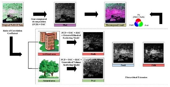
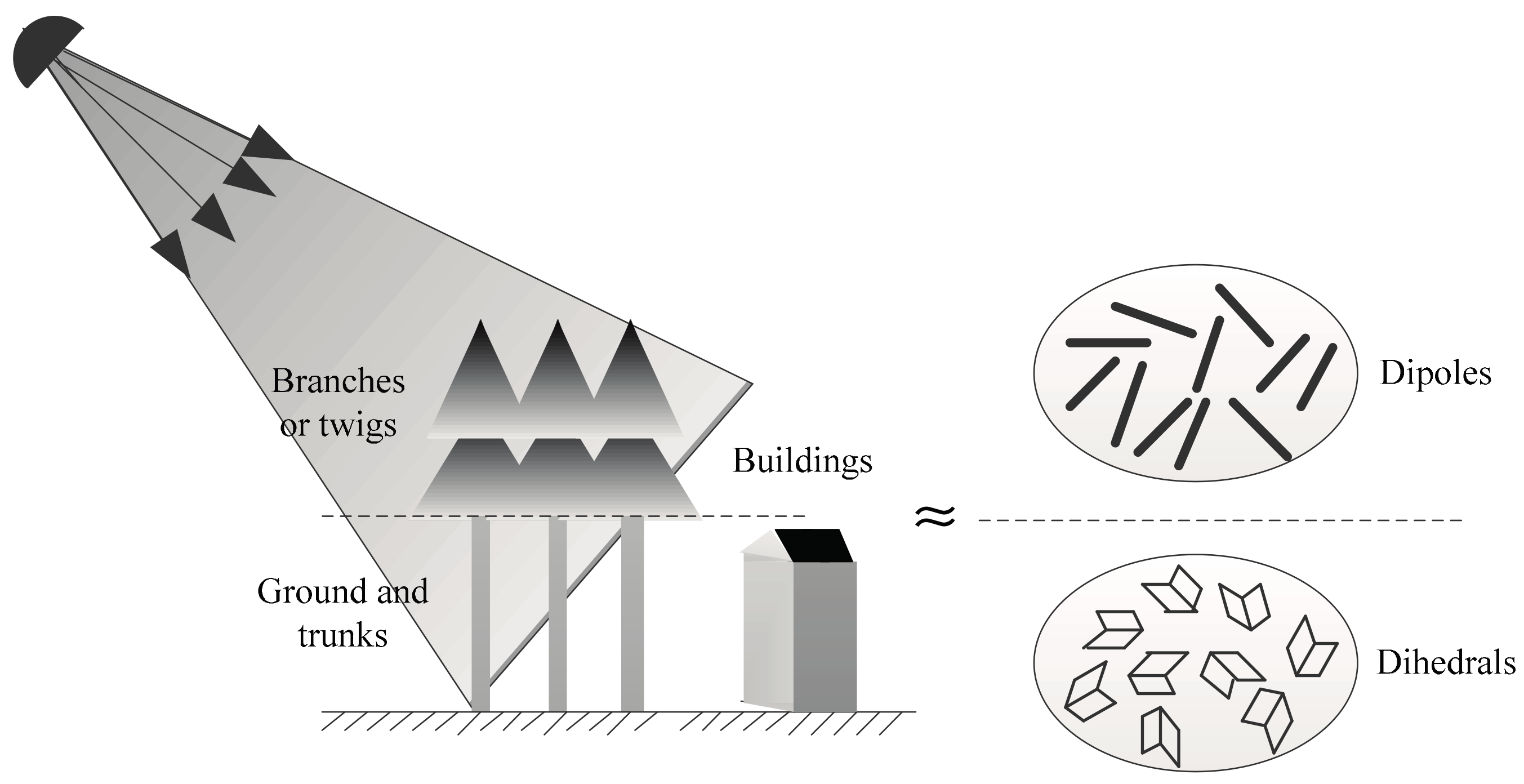
where , , , , and are coefficients to be determined. , , , , and are the specific model corresponding to the surface, double-bounce, volume, oriented dihedral, and helix scattering mechanism, respectively. Other than the G4U, the fourth component is divided into volume scattering and oriented dihedral scattering following some specific criteria. It is known that oriented dihedral scatterings mainly occur in oriented buildings. Additionally, one could consider that the dominant scattering mechanism might be double reflection from the ground-trunk combination for vegetated terrain. They can be regarded as oriented dihedral scatterings as well. As a result, the criteria applied here are used as a way to triage these terrain targets, thus refining the cross-pol component. Their specific expressions are addressed in the following. Schematic representations of the fourth component are given in Figure 1.
In a similar methodology to the G4U, the rotated coherency matrix is then processed by the HAC in order to further account for the real part of , i.e.,
where the subscript represents the rotation according to the helix angle. The oriented dihedral scattering model (the first refined model) and extended matrices are explained as follows. Notice that the HAC has no effect on the helix scattering power since it is applied after the decomposition.
3.1. Oriented Dihedral Scattering Model and Its Extension
The double-bounce scattering mechanism cannot depict urban areas with orientation angles. Therefore, the oriented dihedral scattering model proposed in [8] is used for characterizing these given areas, as shown in
The oriented dihedral scattering model is derived according to the fact that a cosine squared distribution is generally used for vertical structures. The abbreviation is mentioned because the basic scatterer of a building with a nonzero orientation angle is an oriented dihedral corner reflector. It should be noted that when the building orientation angle is 0°, the oriented dihedral scattering model degenerates into the extended model in the G4U. Hence, the oriented dihedral scattering model is theoretically more adaptive than the extended model. The rotated oriented dihedral scattering model is defined as
The elements of are
3.2. Extended Basic Scattering Models
Still, the surface, double-bounce, and helix scattering model in the four-component decomposition [6] are applied. The extended elements of their coherency matrices are expressed as follows.
Surface Scattering Model
Double-bounce Scattering Model
Helix Scattering Model
and denote the shape parameters of surface and double-bounce scattering, respectively.
3.3. Extended Generalized Volume Scattering Model
Instead of the volume scattering model determined by inspection of the ratio between the and terms, we adopt a generalized volume scattering model (GVSM) (the second refined model) for description of the volume scattering contribution in this paper. The GVSM is first proposed by Antropov et al. [22] and has been enriched by several experts and scholars [23,24]. The GVSM is a continuous model covering wide range of co-pol ratio values and can comply with several earlier proposed volume scattering models [5,6]. It is always better to use continuous models as it is unclear what to do especially at the borders when selecting a suitable model. The coherency matrix of the GVSM is given as [22]
where . Therefore, the elements of the extended GVSM can be obtained after the HAC, i.e.,
3.4. Model Inversion
3.4.1. Decomposition Procedure
As mentioned above, the decomposition procedure is hierarchically implemented according to the criteria. If the dominant mechanism is assigned to volume scattering, then the volume scattering model is incorporated into the decomposition. Otherwise, the oriented dihedral scattering model is involved in the decomposition. Here, we use the oriented dihedral scattering model to demonstrate the procedure. After mathematical operations, the relationship between elements of can be rearranged as
From , we can get
Therefore, the coefficients and their relationships can be derived
If the unitary matrix mentioned in the G4U is applied to decomposition with the oriented dihedral scattering model, the corresponding parameters can be calculated in a similar way, i.e.,
After a similar solution and rearrangement, a similar set of equations can be derived with the GVSM, i.e.,
3.4.2. Solution of Underdetermined Equation
It is obvious that expressions in Equations (20) and (22) are underdetermined equation sets. Assumptions need to be predetermined to reduce one of the unknowns. For the four-component decomposition, after subtracting the helix and volume scattering components, there are mainly surface scattering and double-bounce scattering components left in the remaining matrix . For the remaining matrix, the dominant scattering mechanism can be interpreted complying with the principle [24]: if , then the remaining matrix refers to the surface scattering, otherwise refers to the double-bounce scattering ( and are the elements of ). The decision condition can be rearranged as
The decision condition is theoretically more physically straightforward than using the sign of [25]. Take the volume model in the three-component decomposition [5] as an example, the elements of remaining matrix are, respectively, and . As a result, the decision condition is , which is the same as in [26]. If the volume scattering term is omitted, is exactly the one proposed by [22]. Accordingly, the decision condition derived from the GVSM is given as
If , then , assuming the surface scattering is dominant, otherwise , assuming the double-bounce scattering is dominant. Finally, the four-component scattering powers , , (or ), and can be computed as long as the unknowns are determined, thus completing the four-component decomposition.
4. Criteria
4.1. Refined Branch Condition
Before the stage of decomposition, the dominant scattering mechanism within mixed scatterers needs to be predetermined. The purpose of this process is to refine the cross-pol component. In a similar way to the G4U, the assignment of cross-pol components employing the oriented dihedral scattering model is checked as follows.
Under the condition of , the cross-pol component is assigned to a double-bounce scatterer such as a surface-trunk structure or an oriented building. If not, then the dominant mechanism is dipole scattering. Note that when , degenerates into , as applied in the G4U.
4.2. Ratio of Correlation Coefficient
As explained, the refined branch condition can be applied to discriminate the scattering mechanism within mixed scatterers. However, is not suitable for discriminating oriented urban areas since their dominant scattering mechanisms are no longer double-bounce scattering. These areas could be mistakenly classified as natural areas on condition that remains to be incorporated. This may be interpreted as the overestimation of volume scattering in one aspect. In this case, the complex correlation coefficient [27] is considered and the ratio of correlation coefficient (RCC) [28] is adopted to substitute the refined branch condition for its sensibility of scattering characteristics, i.e.,
As is generally known, reflection symmetry is generally present in natural areas and vanishing in artificial areas. Accordingly, the value of for natural areas is approximately zero. In addition, in some artificial areas, the value of is also small for ground objects with strong cross-pol power . Nevertheless, it is found that the numerator and denominator of the RCC change in the opposite trend for the aforementioned areas and natural areas. In this case, natural and artificial areas can be effectively discriminated with the RCC. Based on the aforementioned inference, the criterion for discriminating the areas is given by
where denotes the discriminating threshold. Once judged as artificial areas, the oriented dihedral scattering model is used and the power can be calculated. Otherwise, the generalized volume scattering model is adopted to characterize the volume scattering, thereby can be derived. The flowchart of the proposed method is shown in Figure 2. Power constraints are used to mitigate the problem of negative scattering power.
5. Results and Discussion
The results reported here are derived from the Airborne Synthetic Aperture Radar (AIRSAR), Uninhabited Aerial Vehicle Synthetic Aperture Radar (UAVSAR), Radarsat-2, and the Advanced Land Observing Satellite (ALOS) Phased Array type L-band Synthetic Aperture Radar (PALSAR) polarimetric data acquired over different test sites in San Francisco and San Leandro, United States of America. Several polarimetric analysis techniques are employed.
5.1. Study Site
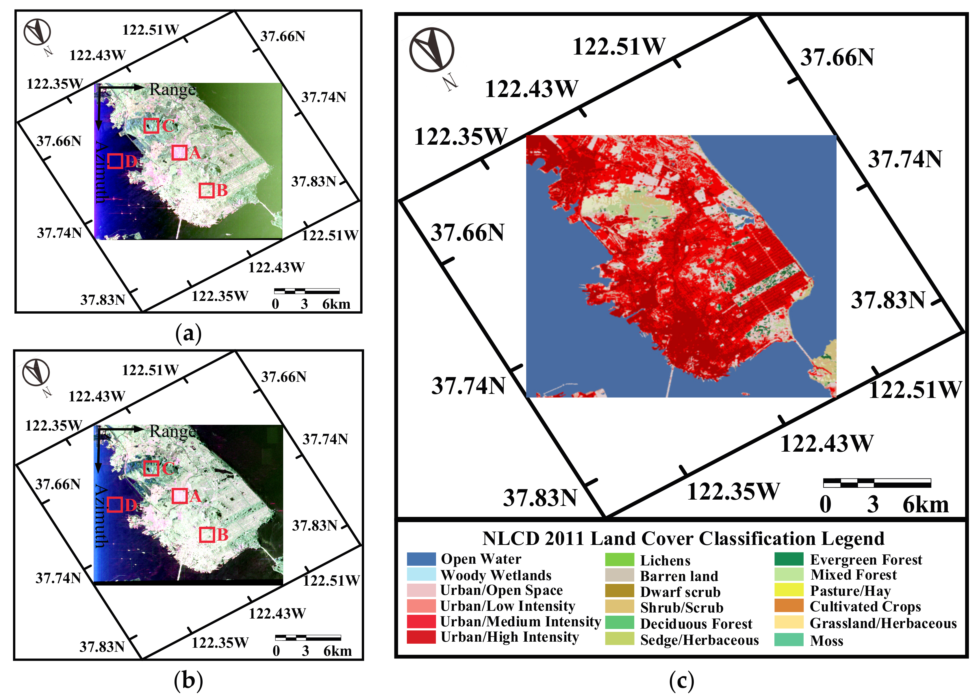
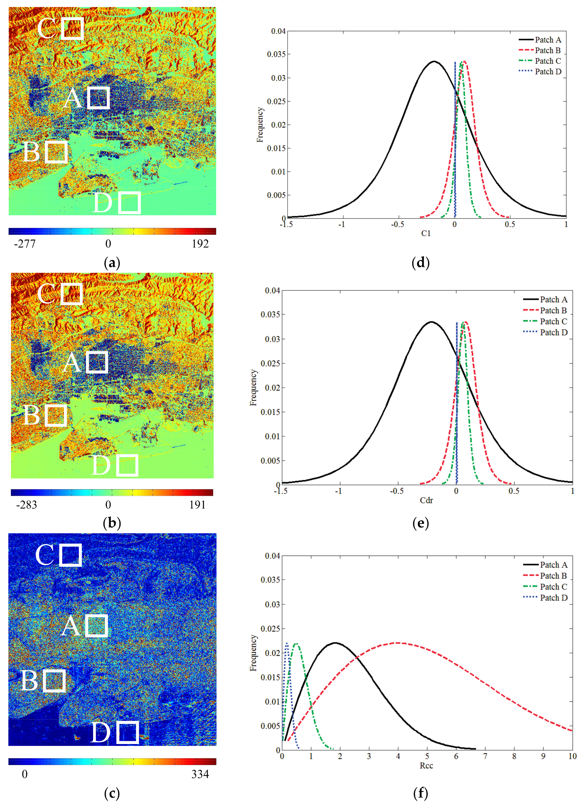
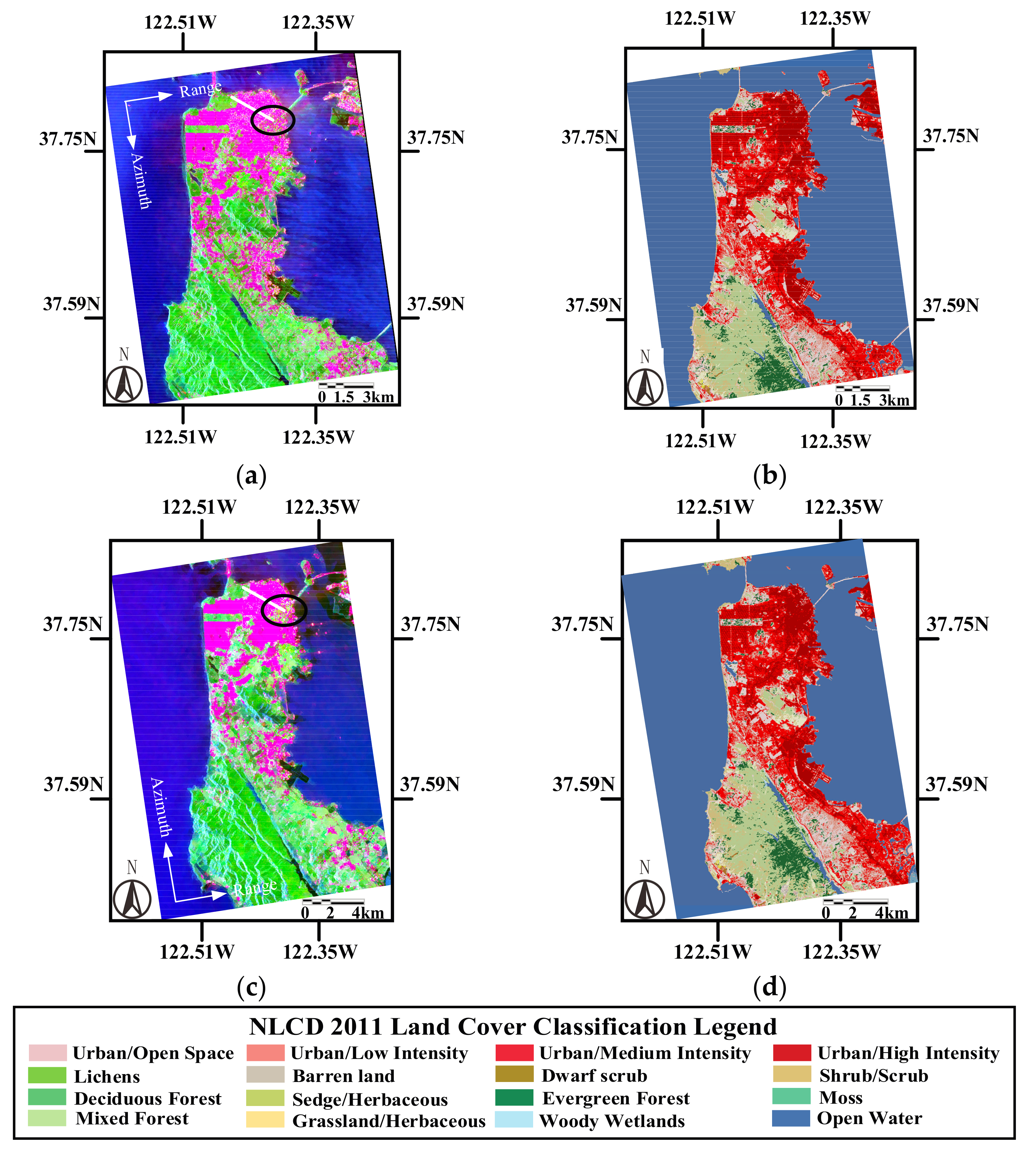
The Pauli color-coded images of AIRSAR C- and L-band data are displayed in Figure 3. The near range and the far range incident angle are 21.5° and 71.4°, respectively. The resolution of the original image corresponds to 6.6 m × 9.3 m in the range and azimuth directions, respectively. The window sizes for the ensemble average in image processing are both chosen as 4 in the range and azimuth direction. In order to evaluate the performance of the proposed method, the National Land Cover Database 2011 (NLCD 2011) is used as the ground reference data, as also shown in Figure 3. NLCD 2011 is the most recent national land cover product created by the Multi-resolution Land Characteristics (MRLC) consortium and it keeps a 16-class land cover classification scheme that has been applied consistently across the United States [29]. Several test sites from the study area are selected to evaluate the experimental results. It consists mainly of orthogonal urban areas (their orientations are almost orthogonal to the radar direction of illumination), oriented urban areas, vegetated terrains, and oceans (patch A, B, C, and D shown in Figure 3, respectively).
5.2. Discriminating Threshold
To ascertain the discriminating threshold, the RCCs of the aforementioned patches are investigated. The averaged NRCC (the numerator of the RCC) and RCC of these patches are shown in Table 1 and Table 2, respectively. As stated in the previous section, the NRCC for natural areas and some special artificial areas is small due to reflection symmetry and intense cross-pol power. This is in accordance with the actual condition from the derived NRCC in Table 1. After the division by the denominator, artificial areas (patch A and patch B) exhibit distinct RCC versus natural areas (patch C and patch D) with regard to different wavebands. There is an obvious segmentation value of the RCC for natural and artificial areas. Accordingly, the discriminating threshold is approximately set as 1.0. Notice that the involved threshold selection is only served as a coarse discrimination of natural and artificial areas. Land covers with specific scattering mechanisms within these two areas need further to be distinguished by the decomposition. More importantly, the related scattering models in the decomposition are used to assign the cross-pol component to volume scattering or oriented dihedral scattering to improve the OVS, which is also the goal of this paper.
5.3. Decomposition Results
The hierarchical extension of general four-component scattering power decomposition (ExG4URcc) developed in this paper is compared both qualitatively and quantitatively with three other approaches—the conventional G4U, the AG4U and the extended G4U (ExG4UCdr, with modifications of the HAC, the refined branch condition, and the oriented dihedral scattering model). All the output results are realized with the same image preprocessing procedure. Empirical power restrictions are used in evaluation of comparative performance of decompositions, and in case that either or is estimated to be negative, they are clipped to zero.
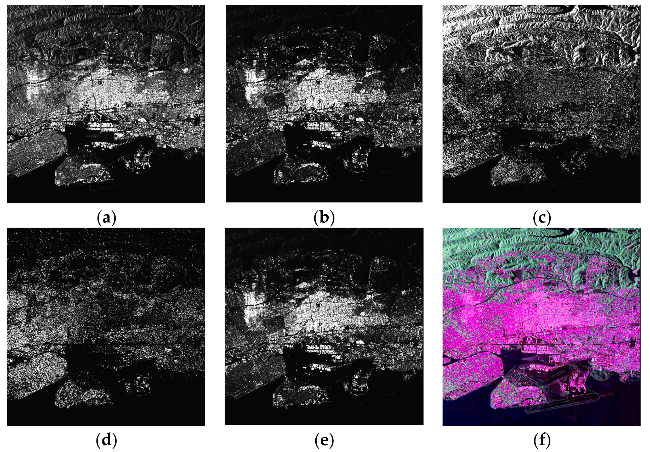
Qualitative Comparison: As an example, the color-coded representations of the G4U, AG4U, ExG4UCdr, and ExG4URcc methods are shown in Figure 4, for which each color brightness corresponds to the magnitude. As expected, volume scattering is the dominating contribution in the total backscatter for vegetated areas. Backscatter for water areas is relatively small, and surface scattering is identified to be dominating for majority of the water pixels with regard to all of the methods. However, it can be seen that the decomposed result derived from the ExG4URcc seems redder, with oriented urban areas identified more clearly, as the level of volume scattering power decreased obviously for them. Moreover, the scattering power from artificial areas (including double bounce scattering power and oriented dihedral scattering power) (red) is enhanced over urban areas and man-made structures with the ExG4URcc. Meanwhile, judging from vast areas in green tone, the OVS exists widely with regard to other methods. Among them, the ExG4UCdr provides redder results over oriented urban areas compared with the G4U and AG4U methods.
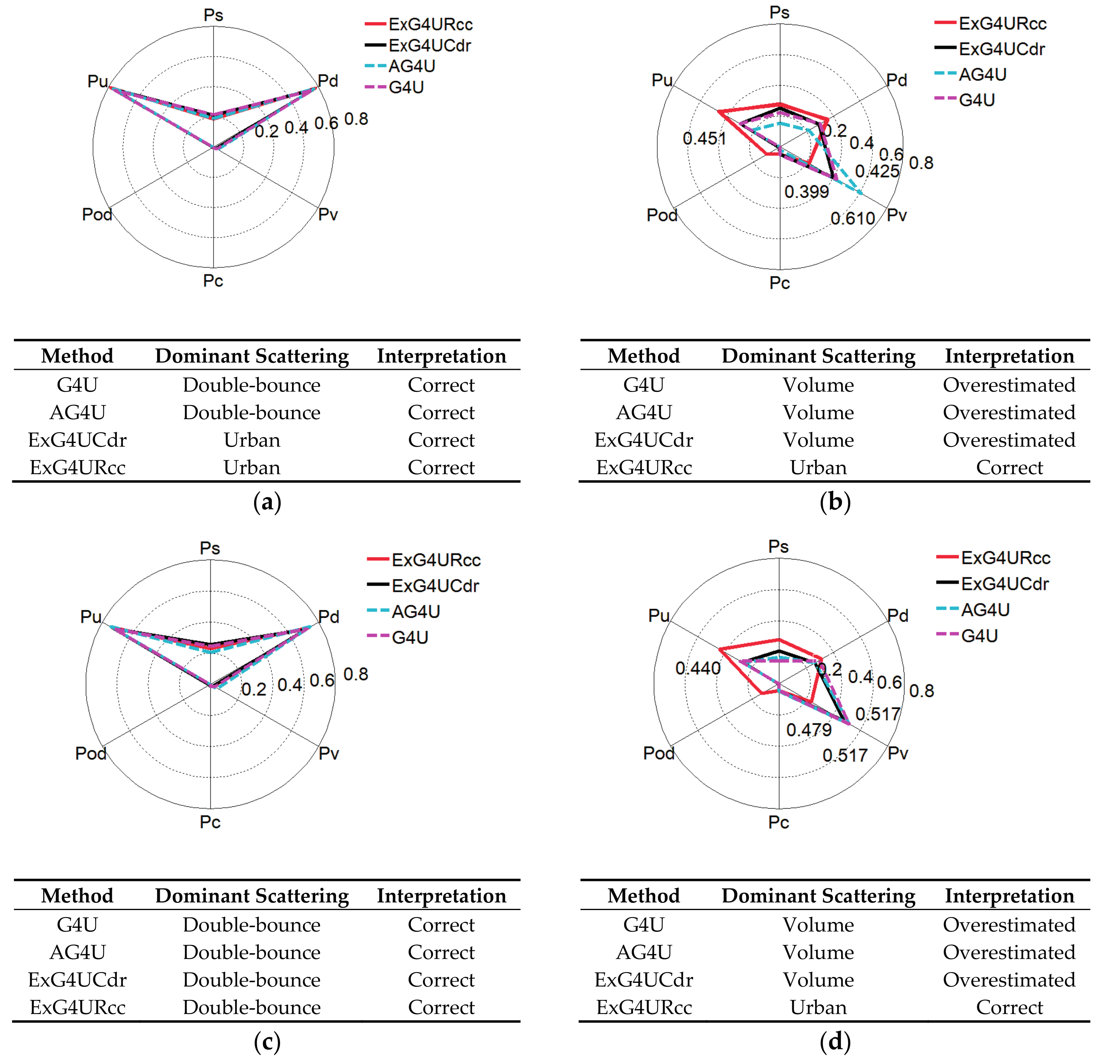
Quantitative Comparison in Different Land Covers: Two kinds of different land covers (see the white and black box areas in Figure 4), including orthogonal urban areas and oriented urban areas are considered for the comparison. Scattering power contributions of , , , , , and are calculated and the relative scale of different scattering powers for these specific urban areas are shown in Figure 5. Each pixel is normalized by the total power of the observation. The tables presented in the bottom indicate the dominant scattering interpreted by the G4U, AG4U, ExG4UCdr, and ExG4URcc methods.
For oriented urban areas, it is noted that derived from the ExG4URcc dramatically enhanced compared with those from other methods for oriented urban areas. Specifically, the scattering power contribution from artificial areas (or the urban scattering power contribution) is increased from 29.9% (in the G4U) to 45.1%, and the oriented dihedral scattering power accounts for 10.1% of the total power, whereas the volume scattering power accounts for only 21.8% of the total power for C-band data. On the one hand, this suggests that the GVSM can appropriately estimate the contribution of volume scattering. On the other hand, it shows that the oriented dihedral scattering matrix can effectively model the cross-pol component from these highly oriented dense urban areas, which results in the occurrence of remarkable oriented dihedral scattering power . Thus, the volume scattering power is significantly decreased with respect to the ExG4URcc. As a result, urban scattering masks volume scattering contribution for majority of these oriented urban pixels. Therefore, the scattering mechanism of the black box areas is identified as having the urban scattering mechanism as dominant. However, for the G4U, AG4U, and ExG4UCdr methods, the dominant scattering mechanisms of the black box areas are all regarded as volume scattering with regard to each waveband. For instance, their corresponding volume scattering powers are 0.517, 0.517, and 0.479 for L-band data, respectively. This indicates that these three methods still suffer the deficiency of the OVS as well as erroneous interpretation. In addition, notice that all of the lines almost coincide in the left column of Figure 6. This indicates that similar decomposition results obtain as for orthogonal urban areas, as majority of pixels exhibits urban scattering behavior. As a result, the detailed quantitative comparisons will not be discussed for this land cover.
Figure 6 gives a more intuitive illustration that the urban scattering dominant characteristics are marked red. As previous mentioned, in contrast to the G4U and AG4U methods, more reddish results happen with the ExG4UCdr due to the increment of surface, double-bounce, and oriented dihedral scattering. This is reasonable since the red box areas are covered with buildings and streets. Consequently, the volume scattering obtained by the ExG4UCdr is not too overestimated, which is ascribed to the incorporation of the aforementioned modifications. Despite all of this, these modifications only lead to partial improvements in the results. Otherwise, the overestimation of volume scattering can be solved via the ExG4UCdr. Therefore, they are not the main sources of enhancement.
To further examine the scattering powers of the proposed method, the extent of scattering components’ change with different waveband data has been investigated. Since the objective is to ameliorate the overestimation of volume scattering, only oriented urban areas are involved. The corresponding normalized volume and oriented dihedral scattering power statistics are shown in Table 3 and Table 4. It is seen that the volume scattering power turns intense with the increase in wavelengths with the exception of the L-band result derived from the AG4U. The results of the two frequencies are probably related to the different relative weights of and , dictated by the different sensed relative roughness. In Table 4, it can also be seen that the oriented dihedral scattering enhances as the wavelength increases with the ExG4URcc. A plausible explanation is that the induced cross-pol return is more intense when the lower frequency radiation acts on an oblique building. It is known that the differences between the G4U and ExG4UCdr methods are the HAC, the refined branch condition, and the oriented dihedral scattering model. In Table 3, it can be seen that with the ExG4UCdr, the volume scattering power respectively decreases by 2.6% and 3.8% compared with the G4U. Meanwhile, the oriented dihedral scattering power respectively accounts for 0.9% and 0.6% of the total power. This demonstrates that the oriented dihedral scattering model make a partial contribution to the decrement of volume scattering power. The rest is benefit from the incorporation of the HAC and the refined branch condition. These two modifications will be discussed in the following.
5.4. Performance of the HAC
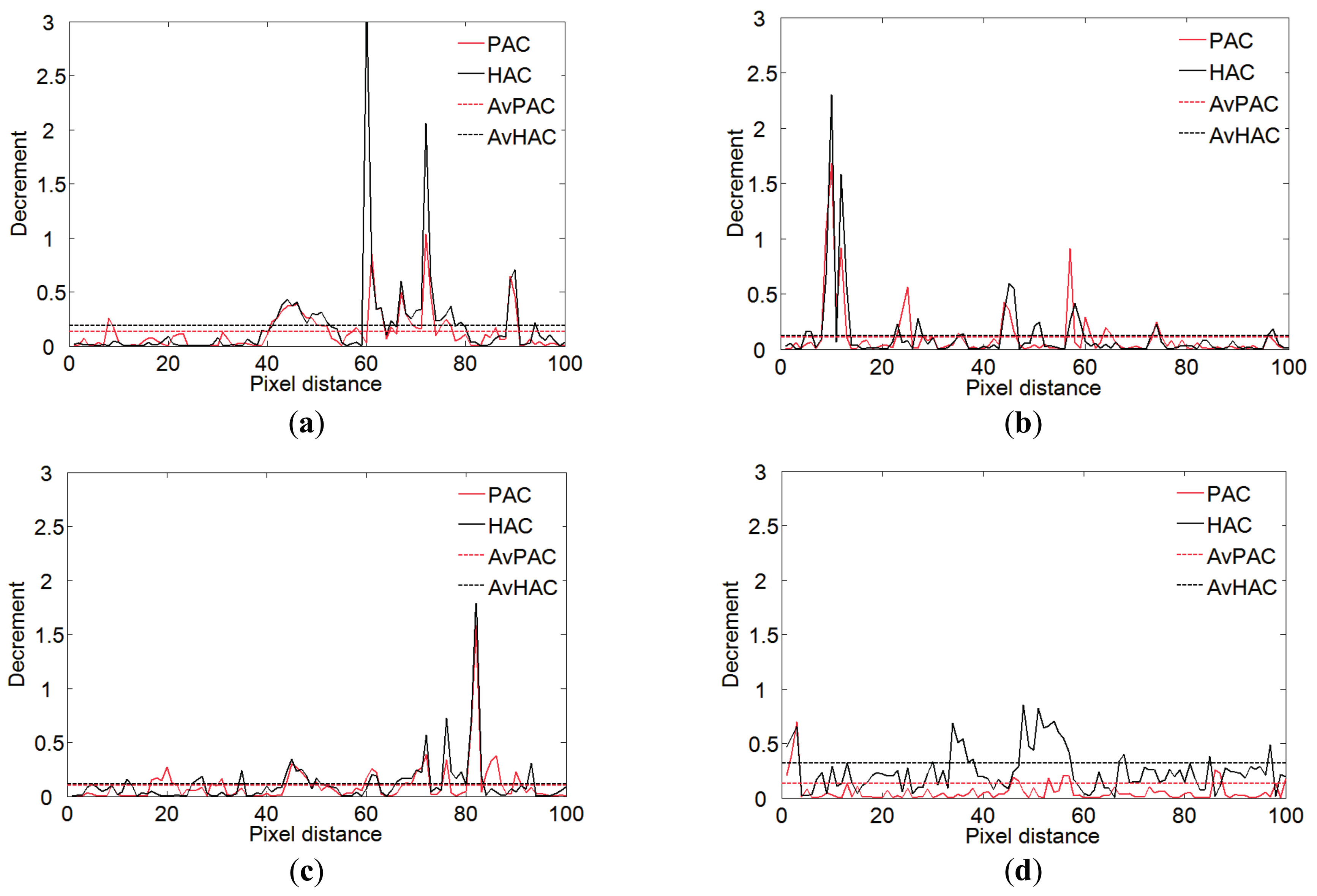
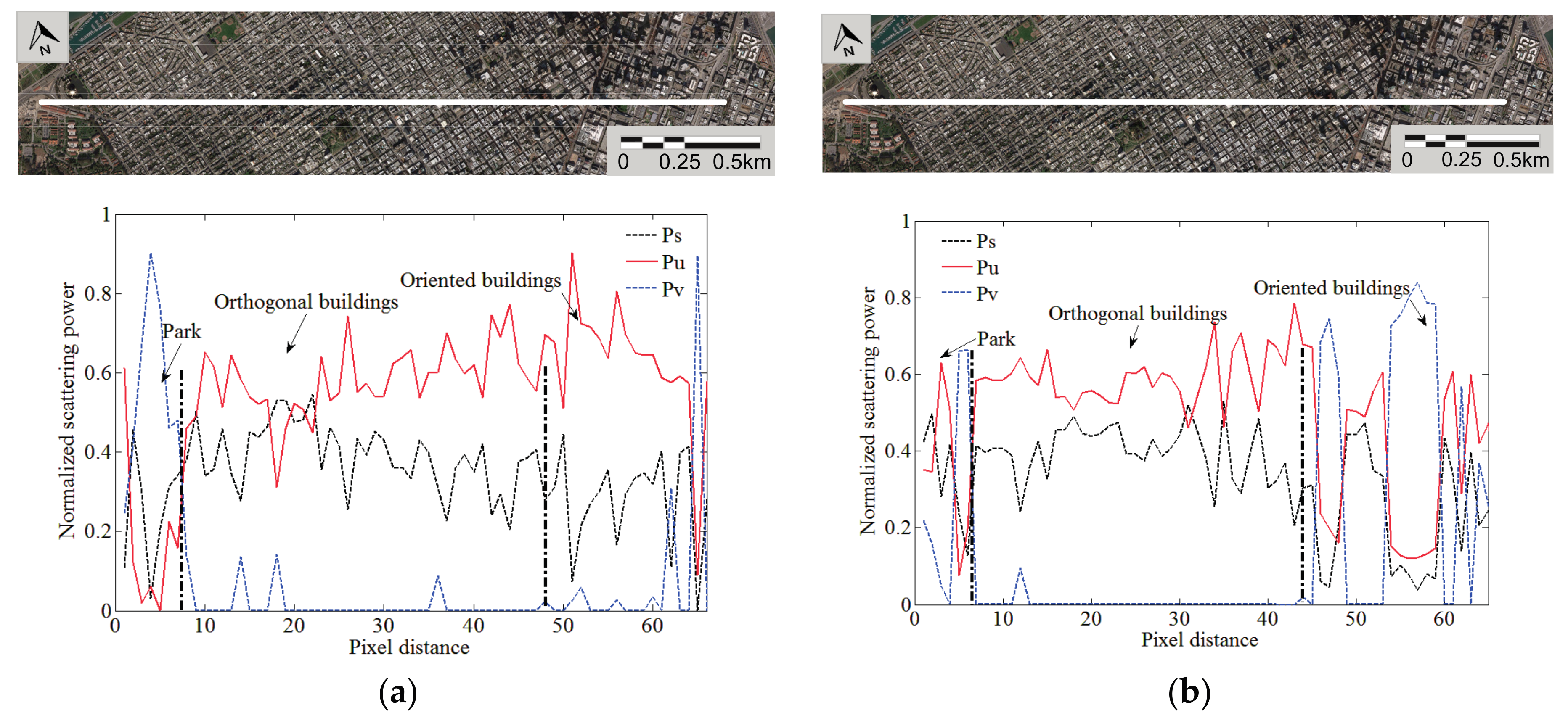
Without loss of generality, two lists of pixels (see the white and black lines in Figure 4) are selected from the aforementioned urban areas to evaluate the performances of different angle compensations. Only the PAC and HAC are involved in the comparison since the OAC is applied beforehand. The decrements of the term for the PAC and HAC are computed and shown in Figure 7. The red and black dotted lines represent the averaged decrement of the term for the PAC and HAC, respectively. Notice that the decrements for the PAC and HAC are quite small since the OAC already reduces a large amount of cross-pol power. Moreover, the term continues to decrease via the PAC and HAC as long as the OAC is done correctly. It can be seen that the red dotted line is always beneath the black dotted line. Given this, we can conclude that the HAC advantages itself in reducing the term compared with the PAC. This is one aspect of proving that the proposed method can effectively impair the volume scattering with the HAC.
Another concern associated with model-based decompositions is the occurrence of negative scattering powers. The occurrence of negative scattering powers generally happens to surface or double-bounce scattering since contributions of the volume or helix scattering are first estimated from the total measured data. The percentage of negative scattering powers has been investigated for two different circumstances: (1) or ; and (2) both and . As seen in Table 5 and Table 6, the percentages of negative scattering powers have been reduced by 6.2% and 12.6%, respectively, from the G4U to the ExG4URcc under Circumstance (1), while, for Circumstance (2), there are decreases of 15.4% and 3.1% from the G4U to the ExG4URcc, respectively. This indicates that negative scattering powers are drastically reduced with the ExG4URcc. Furthermore, the ExG4URcc always achieves the minimum percentage of negative scattering powers for both of the wavebands. In addition, it is also known that the ExG4URcc performs better in reducing the negative scattering powers for L-band data since the percentages of negative scattering powers are the smallest for both of the circumstances (2.7% and 3.3%).
On the other hand, it is known that the HAC has better performance in the reduction of the term, which can actually bring about the relaxation of the OVS. Consequently, the volume scattering power can be constrained not to exceed the total power to a certain extent, thus lowering the chance that surface scattering power (or double-bounce scattering power) becomes negative. This inference can be confirmed from the total percentages obtained by the ExG4UCdr and ExG4URcc methods since the HAC is applied throughout the procedure (e.g., 7.3% and 6.0% for L-band data). Therefore, it is more inclined to employ the HAC instead of the PAC based on the above conclusion.
5.5. Comparison of Criteria
The second PolSAR data are acquired by UAVSAR over another test site in San Leandro, as shown in Figure 8a, and have coverage of orthogonal and oriented buildings, and natural targets such as woods and ocean. Figure 8b displays the fully polarimetric UAVSAR L-band data with Pauli color coding. The original PolSAR data are acquired on 20 November 2014 and have a resolution with 7.2 m in azimuth direction and 5 m in range direction.
In order to compare the performance of different criteria, we give the magnitudes of , , and , as shown in the left column of Figure 9. Four test patches corresponding to orthogonal buildings (A), oriented buildings (B), woods (C), and ocean (D) are selected from the magnitude images for evaluation. The fitting histograms of these areas are shown in the right column of Figure 9. In Figure 9f, it can be seen that performs much better than other criteria since the magnitude difference between natural and artificial areas is apparent. The buildings in patch A and patch B exhibit much larger RCCs compared with other land covers, making them be easily discriminated from natural areas using the discriminating threshold. However, regards oriented buildings in Figure 9d,e, they are mixed up with woods because of the similar magnitude values. In addition, notice that oriented buildings present more positive values in and . This implicates that they cannot be effectively distinguished using or . As discussed in the G4U, the assignment of cross-pol component depends on the sign of . In fact, only represents a special case of which meets the condition of . Hence, it is reasonable to deduce that can be used to identify more pixels with double-bounce scattering.
To give a quantitative comparison, statistics of whole image pixels processed by these criteria are given in Table 7. The size of the UAVSAR L-band image is 500 pixels × 500 pixels. It is seen that pixels processed by the RCC are approximately twice as many as those processed by and . This explains that the RCC is advantageous in discrimination of natural and artificial areas. In addition, the relationship of pixel numbers between and verifies the aforementioned deducing. As stated earlier, the HAC and the refined models are not the main sources of enhancement (recall the GVSM is only applied to natural areas), whereas, by integrating the RCC, hierarchical decompositions with the refined models are implemented, thus the overestimation problem can be overcome. Hence, the enhancement is mainly attributed to the introduction of the RCC. Despite all of this, it should be noted that the improvement is resulting from interactions among the modifications in the proposed method.
Figure 10 presents the decomposition results of the proposed method. In Figure 10b, we can see that double-bounce scattering powers from orthogonal buildings are very strong, whereas those from buildings with large orientation angles are low. Meanwhile, oriented buildings have strong oriented dihedral scattering powers, as shown in Figure 10d. Notice that some woods also have low oriented dihedral scattering powers. This is because double reflections from the ground-trunk combination can be identified due to the considerable penetration of L-band. In Figure 10b,e, it can be found that the difference between double-bounce scattering and urban scattering is small. This suggests that oriented dihedral scattering is weak compared to double-bounce scattering. Figure 10f shows the decomposed color-coded composite image. What we can see is that the red color of orthogonal buildings is brighter than that of oriented buildings. Even so, oriented urban areas still can be identified. This highlight of red color serves to interpret the dominant scattering mechanism of oriented urban areas more clearly.
To validate the performance of the ExG4URcc, the same patches (see the white box areas in Figure 9) are selected from the scene for quantitative comparisons among other methods. In Figure 11, we can see that for orthogonal buildings, woods, and ocean, the dominant scattering mechanisms are all correctly interpreted. Nevertheless, regards these three kinds of land covers, the volume scattering power derived from the ExG4URcc is always the smallest (e.g., 0.021, 0.437, and 0.052, respectively). This explains that the proposed method can effectively reduce the volume scattering, thus lowering the risk of the occurrence of the OVS. For oriented buildings, it can be seen that the volume scattering power is significantly smaller than the urban scattering power. Meanwhile the surface scattering component of the ExG4URcc is increased, as compared with those of other methods. In spite of this, the urban scattering is still larger than the surface scattering power. As a result, the dominant scattering mechanism of these areas is considered as urban scattering, which is conformity with the reality. However, for the G4U and AG4U methods, the results disclose the phenomenon that the volume scattering is still overestimated. It is worth noting that according to the magnitude relationship of the double-bounce and volume scattering powers (0.321 versus 0.318) derived from the ExG4UCdr, the dominant scattering mechanism can already be identified as urban scattering, let alone the existing oriented dihedral scattering powers. As mentioned above, the refined branch condition embedded in the ExG4UCdr plays a role in reducing the volume scattering. This indicates that the ExG4UCdr can also improve the OVS for some specific oriented urban areas.
5.6. Results with Spaceborne Data
Finally, we apply the proposed method to two sets of spaceborne data. These data are, respectively, acquired by Radarsat-2 and ALOS PALSAR over the same area in San Francisco. For estimating the coherency matrix, the multilook processing is performed in the preprocessing of the data. The final resolution is 23.7 m × 24.1 m and 21.2 m × 28.1 m in the ground area for Radarsat-2 and ALOS PALSAR images, respectively.
Based on the proposed decomposition, a color composite image showing the dominant scattering mechanism in each area is generated, as shown in Figure 12. Still, the scattering component from artificial areas (red) contains contribution from both the double-bounce and oriented dihedral observations in the image. Overall, the ocean and airport runway areas are surface scattering dominant, while some coastal waters appear black due to specular reflection. The mountainous areas covered with forests are dominated by volume scattering. With the proposed method, improved performance is achieved especially in terrain consisting of oriented buildings (the black ellipse areas). As a result, the built-up areas are dominated by double-bounce or oriented dihedral scattering.
To further test the validity of the proposed approach, a transect shown in white line in Figure 12 is made to show profiles of the decomposition power. This transect includes the park, orthogonal urban areas, and oriented urban areas. Therefore, land cover variation can be recognized. The values of the decomposed powers along the transect are calculated, resulting in Figure 13. It reflects the status of each of the scattering mechanisms. From the inspection of Figure 13, it can be see that the contribution of agrees with the distribution of both orthogonal and oriented urban areas. However, one may find out that some pixels in oriented urban areas exhibit strong volume scattering from the tail end of these curves. This situation occurs due to the following two reasons. On the one hand, discriminations of oriented buildings are not so accurate since the discriminating threshold is empirically determined. One the other hand, the oriented dihedral scattering model is found to inappropriately characterize those buildings with smaller orientation angles. These remaining problems will be considered in the future study.
6. Conclusions
For urban areas, due to the high variability of urban landscape and its wide variety of constructions, their polarimetric scattering mechanisms are more complicated with respect to natural areas. As one of the intrinsic drawbacks, the overestimation of volume scattering severely impairs the performance of model-based decomposition. The major cause can be summarized as follows: (1) in most of decomposition methods, the cross-pol return is assumed as only from volume scattering; (2) the oriented dihedral scattering from buildings that not aligned facing the radar look direction has the nonzero orientation angle and thus induces cross-pol returns; and (3) a misinterpretation occurs between oriented urban areas and natural areas since they are contributed by the cross-pol power as well. In this case, it is desirable to distinguish these scattering mechanisms for accurate classification since they exhibit similar polarimetric responses.
In this paper, an extension of the Singh’s general four-component decomposition is proposed, which provides a new method to discriminate these mixed areas and improve the overestimation of volume scattering. In a similar way to the G4U, the derivation of scattering coefficients based on the HAC is presented. Moreover, the RCC shifts versus different land covers are explored, thus obtaining the threshold for discriminating natural and artificial areas. Finally, the decomposition is hierarchically implemented and the corresponding scattering power is calculated. Different waveband data sets acquired by AIRSAR, UAVSAR, Radarsat-2, and ALOS PALSAR are used to verify the inferences. Several urban area patches with different building orientations are selected. The involved modifications are discussed and compared, thus reaching the conclusion that the RCC contribute most to the enhancement. From the estimated volume and urban scattering component in patches, the OVS problem has been improved in real earnest and the scattering mechanism ambiguity no longer exist in oriented urban areas.
Acknowledgments
This work is supported by the National Natural Science Foundation of China under Grant 61401477.
Author Contributions
Sinong Quan is responsible for the design of the methodology, experimental data collection and processing, and preparation of the manuscript. Deliang Xiang, Boli Xiong, and Canbin Hu helped analyze and discuss the results. Gangyao Kuang is responsible for the technical support of the manuscript.
Conflicts of Interest
The authors declare no conflict of interest.
References
- Sugimoto, M.; Ouchi, K.; Nakamura, Y. Four-Component Scattering Power Decomposition Algorithm with Rotation of Covariance Matrix Using ALOS-PALSAR Polarimetric Data. Remote Sens. 2012, 4, 2199–2209. [Google Scholar] [CrossRef]
- Xie, Q.; Ballester-Berman, J.D.; Lopez-Sanchez, J.M.; Zhu, J.; Wang, C. Quantitative Analysis of Polarimetric Model-Based Decomposition Methods. Remote Sens. 2016, 8, 977. [Google Scholar] [CrossRef]
- Xiang, D.; Tang, T.; Ban, Y.; Su, Y.; Kuang, G. Unsupervised polarimetric SAR urban area classification based on model-based decomposition with cross scattering. ISPRS J. Photogramm. Remote Sens. 2016, 116, 86–100. [Google Scholar] [CrossRef]
- Xi, Y.; Lang, H.; Tao, Y.; Huang, L.; Pei, Z. Four-Component Model-Based Decomposition for Ship Targets Using PolSAR Data. Remote Sens. 2017, 9, 621. [Google Scholar] [CrossRef]
- Freeman, A.; Durden, S.L. A three-component scattering model for polarimetric SAR data. IEEE Trans. Geosci. Remote Sens. 1998, 36, 963–973. [Google Scholar] [CrossRef]
- Yamaguchi, Y.; Moriyama, T.; Ishido, M.; Yamada, H. Four-component scattering model for polarimetric SAR image decomposition. IEEE Trans. Geosci. Remote Sens. 2005, 43, 1699–1706. [Google Scholar] [CrossRef]
- Zhang, L.; Zou, B.; Cai, H.; Zhang, Y. Multiple-Component Scattering Model for Polarimetric SAR Image Decomposition. IEEE Geosci. Remote Sens. Lett. 2008, 5, 603–607. [Google Scholar] [CrossRef]
- Xiang, D.; Ban, Y.; Su, Y. Model-Based Decomposition With Cross Scattering for Polarimetric SAR Urban Areas. IEEE Geosci. Remote Sens. Lett. 2015, 12, 2496–2500. [Google Scholar] [CrossRef]
- Lee, J.S.; Ainsworth, T.L.; Wang, Y. Generalized polarimetric model-based decompositions using incoherent scattering models. IEEE Trans. Geosci. Remote Sens. 2014, 52, 2474–2491. [Google Scholar] [CrossRef]
- Arii, M.; van Zyl, J.J.; Kim, Y. Adaptive model-based decomposition of polarimetric SAR covariance matrices. IEEE Trans. Geosci. Remote Sens. 2011, 49, 1104–1113. [Google Scholar] [CrossRef]
- Arii, M.; van Zyl, J.J.; Kim, Y. A General Characterization for Polarimetric Scattering From Vegetation Canopies. IEEE Trans. Geosci. Remote Sens. 2010, 48, 3349–3357. [Google Scholar] [CrossRef]
- Van Zyl, J.J.; Arii, M.; Kim, Y. Model-based decomposition of polarimetric SAR covariance matrices constrained for nonnegative eigenvalues. IEEE Trans. Geosci. Remote Sens. 2011, 49, 3452–3459. [Google Scholar] [CrossRef]
- Cui, Y.; Yamaguchi, Y.; Yang, J.; Kobayashi, H.; Park, S.E.; Singh, G. On complete model-based decomposition of polarimetric SAR coherency matrix data. IEEE Trans. Geosci. Remote Sens. 2014, 52, 1991–2001. [Google Scholar] [CrossRef]
- An, W.; Cui, Y.; Yang, J. Three-Component Model-Based Decomposition for Polarimetric SAR Data. IEEE Trans. Geosci. Remote Sens. 2010, 48, 2732–2739. [Google Scholar] [CrossRef]
- Lee, J.S.; Ainsworth, T.L. The Effect of Orientation Angle Compensation on Coherency Matrix and Polarimetric Target Decompositions. IEEE Trans. Geosci. Remote Sens. 2011, 49, 53–64. [Google Scholar] [CrossRef]
- Yamaguchi, Y.; Sato, A.; Boerner, W.-M.; Sato, R.; Yamada, H. Four-Component Scattering Power Decomposition With Rotation of Coherency Matrix. IEEE Trans. Geosci. Remote Sens. 2011, 49, 2251–2258. [Google Scholar] [CrossRef]
- An, W.; Xie, C.; Yuan, X.; Cui, Y.; Yang, J. Four-component decomposition of polarimetric SAR images with deorientation. IEEE Geosci. Remote Sens. Lett. 2011, 8, 1090–1094. [Google Scholar] [CrossRef]
- Chen, S.W.; Ohki, M.; Shimada, M.; Sato, M. Deorientation effect investigation for model-based decomposition over oriented built-up areas. IEEE Geosci. Remote Sens. Lett. 2013, 10, 273–277. [Google Scholar] [CrossRef]
- Singh, G.; Yamaguchi, Y.; Park, S.E. General four-component scattering power decomposition with unitary transformation of coherency matrix. IEEE Trans. Geosci. Remote Sens. 2013, 51, 3014–3022. [Google Scholar] [CrossRef]
- Sato, A.; Yamaguchi, Y.; Singh, G.; Park, S.E. Four-component scattering power decomposition with extended volume scattering model. IEEE Geosci. Remote Sens. Lett. 2012, 9, 166–170. [Google Scholar] [CrossRef]
- Bhattacharya, A.; Singh, G.; Manickam, S.; Yamaguchi, Y. An adaptive general four-component scattering power decomposition with unitary transformation of coherency matrix (AG4U). IEEE Geosci. Remote Sens. Lett. 2015, 12, 2110–2114. [Google Scholar] [CrossRef]
- Antropov, O.; Rauste, Y.; Häme, T. Volume scattering modeling in PolSAR decompositions: Study of ALOS PALSAR data over boreal forest. IEEE Trans. Geosci. Remote Sens. 2011, 49, 3838–3848. [Google Scholar] [CrossRef]
- Xie, Q.; Ballester-Berman, D.; Lopez-Sanchez, J.M.; Zhu, J.; Wang, C. On the Use of Generalized Volume Scattering Models for the Improvement of General Polarimetric Model-Based Decomposition. Remote Sens. 2017, 9, 117. [Google Scholar] [CrossRef]
- Xiang, D.; Wang, W.; Tang, T.; Su, Y. Multiple-component polarimetric decomposition with new volume scattering models for PolSAR urban areas. IET Radar Sonar Navig. 2017, 11, 410–419. [Google Scholar] [CrossRef]
- An, W.; Xie, C. An improvement on the complete model-based decomposition of polarimetric SAR data. IEEE Geosci. Remote Sens. Lett. 2014, 11, 1926–1930. [Google Scholar] [CrossRef]
- Yajima, Y.; Yamaguchi, Y.; Sato, R.; Yamada, H.; Boerner, W.-M. POLSAR Image Analysis of Wetlands Using a Modified Four-Component Scattering Power Decomposition. IEEE Trans. Geosci. Remote Sens. 2008, 46, 1667–1673. [Google Scholar] [CrossRef]
- Ratha, D.; Surender, M.; Bhattacharya, A. Improvement of PolSAR Decomposition Scattering Powers Using a Relative Decorrelation Measure. Remote Sens. Lett. 2017, 8, 340–349. [Google Scholar] [CrossRef]
- Xiang, D.; Tang, T.; Hu, C.; Fan, Q.; Su, Y. Built-up area extraction from PolSAR imagery with model-based decomposition and polarimetric coherence. Remote Sens. 2016, 8, 685. [Google Scholar] [CrossRef]
- Jin, S.; Yang, L.; Danielson, P.; Homer, C.; Fry, J.; Xian, G. A Comprehensive Change Detection Method for Updating the National Land Cover Database to Circa 2011. Remote Sens. Environ. 2013, 132, 159–175. [Google Scholar] [CrossRef]
Figure 1.
Division of the fourth component.

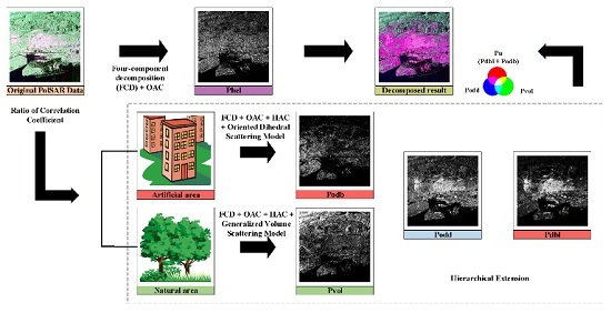
Figure 2.
General scheme of the proposed method.
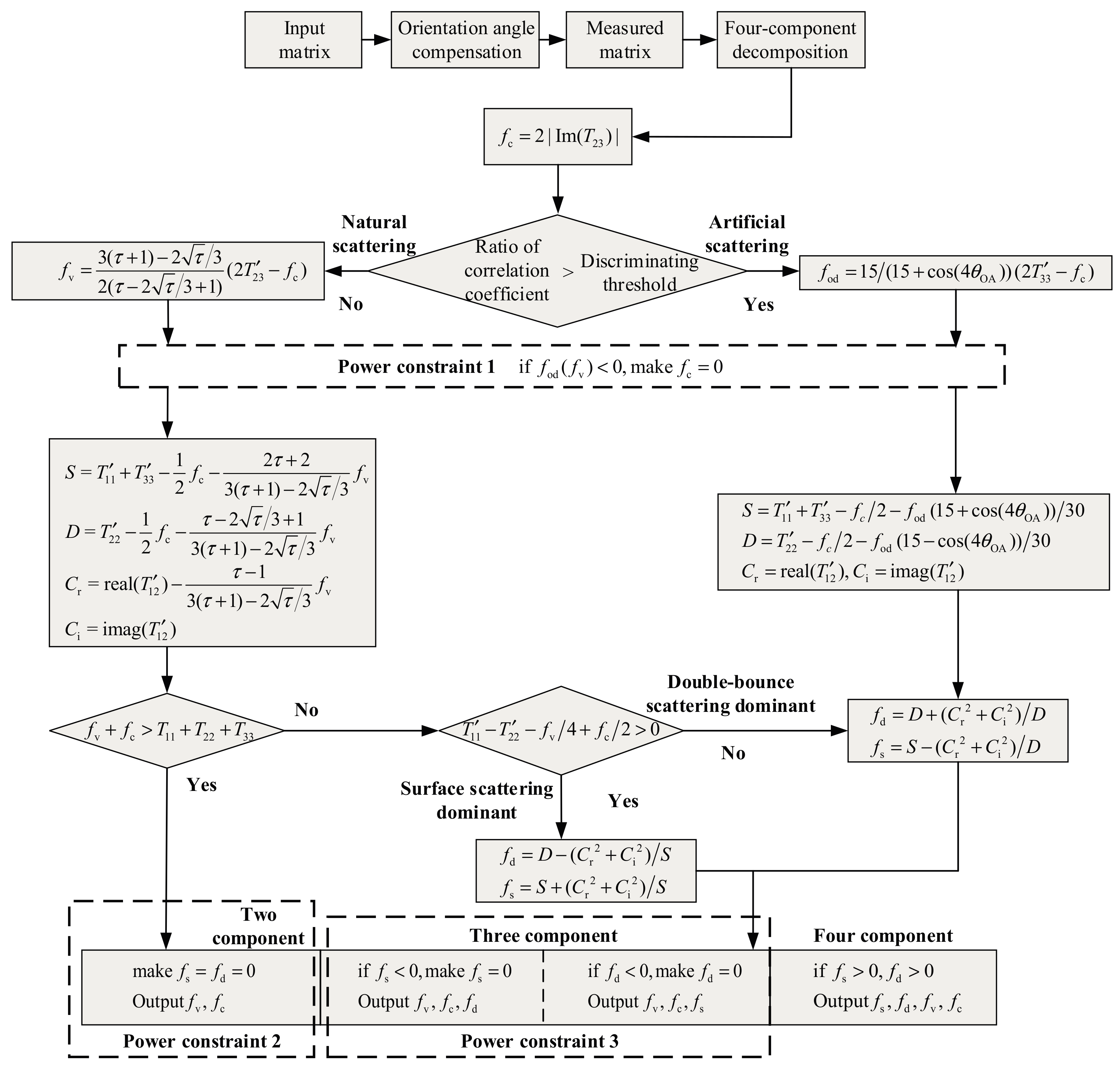
Figure 3.
Pauli decomposition of PolSAR data and selected patches in the test site: (a) C-band data; (b) L-band data; and (c) ground reference of San Francisco.
Figure 3.
Pauli decomposition of PolSAR data and selected patches in the test site: (a) C-band data; (b) L-band data; and (c) ground reference of San Francisco.

Figure 4.
Color-coded scattering power decomposition with red (urban scattering), green (volume scattering), and blue (surface scattering): (a–d) decomposition results for C-band data using the conventional general four-component scattering power decomposition (G4U), the adaptive G4U (AG4U), the extended G4U (ExG4UCdr), and the hierarchical extended G4U (ExG4URcc) methods, respectively; and (e–h) decomposition results for L-band data using the G4U, AG4U, ExG4UCdr, and ExG4URcc methods, respectively.
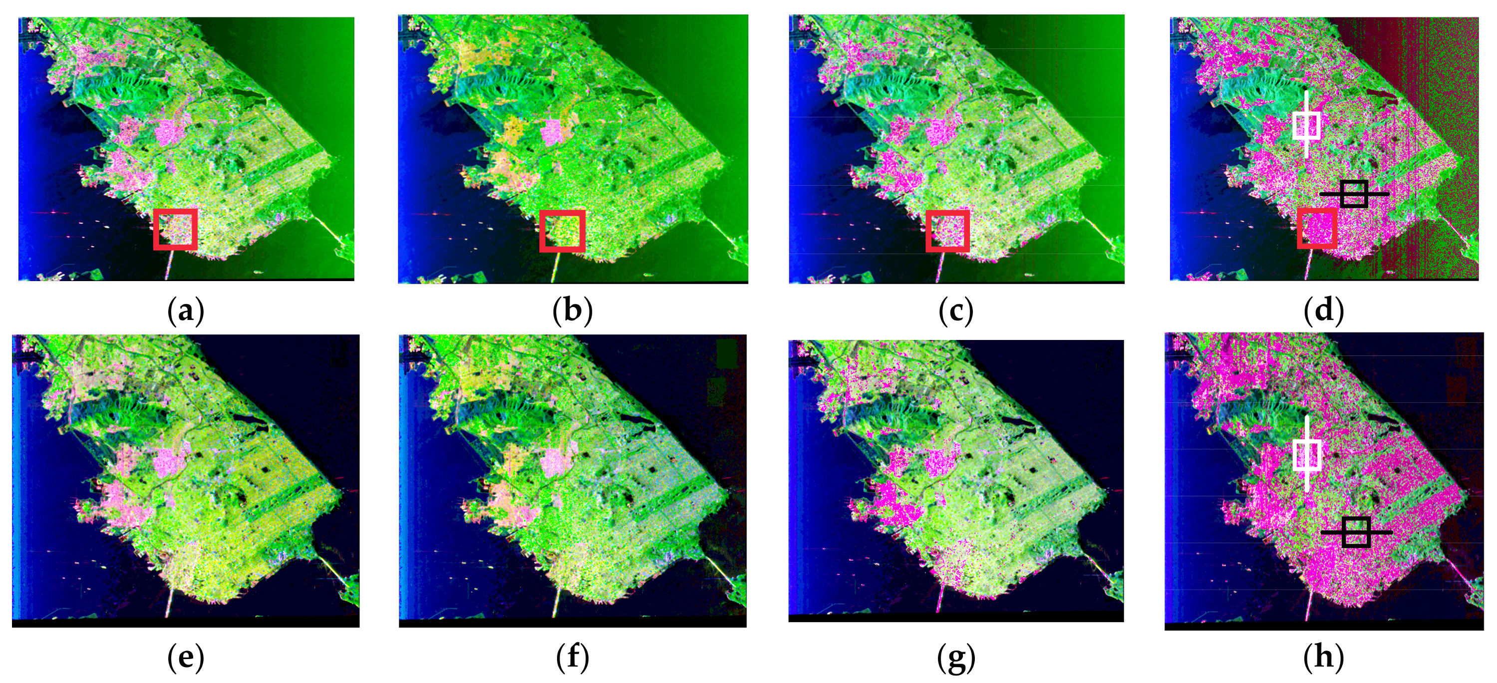
Figure 5.
Radar map of averaged power contribution: (a,b) results of the white box areas derived from C- and L-band data, respectively; and (c,d) results of the white box areas derived from C- and L-band data, respectively.
Figure 5.
Radar map of averaged power contribution: (a,b) results of the white box areas derived from C- and L-band data, respectively; and (c,d) results of the white box areas derived from C- and L-band data, respectively.

Figure 6.
Enlarged fragments of color-coded representations of decomposed red box areas in Figure 4 using the: (a) G4U; (b) AG4U; (c) ExG4UCdr; and (d) ExG4URcc methods; and (e) the corresponding optical image. Courtesy: Google earth.
Figure 6.
Enlarged fragments of color-coded representations of decomposed red box areas in Figure 4 using the: (a) G4U; (b) AG4U; (c) ExG4UCdr; and (d) ExG4URcc methods; and (e) the corresponding optical image. Courtesy: Google earth.
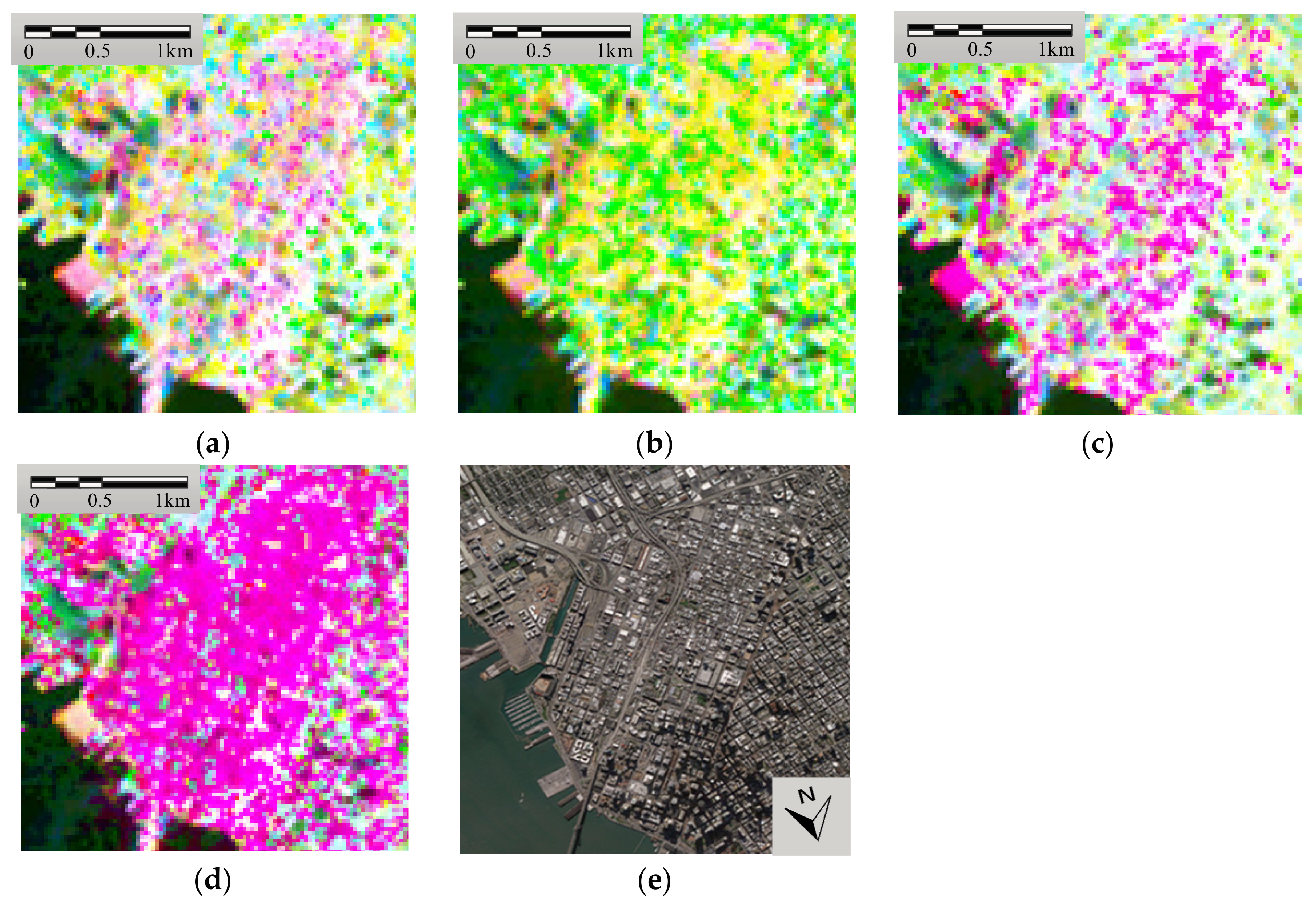
Figure 7.
Decrements of the term via different angle compensations on the selected lines: (a,b) decrements along the white line for C- and L-band data, respectively; and (c,d) decrements along the black line for C- and L-band data, respectively.
Figure 7.
Decrements of the term via different angle compensations on the selected lines: (a,b) decrements along the white line for C- and L-band data, respectively; and (c,d) decrements along the black line for C- and L-band data, respectively.

Figure 8.
Second study area and UAVSAR data: (a) ground reference (NLCD 2011); and (b) Pauli-coded SAR image with L-band.
Figure 8.
Second study area and UAVSAR data: (a) ground reference (NLCD 2011); and (b) Pauli-coded SAR image with L-band.
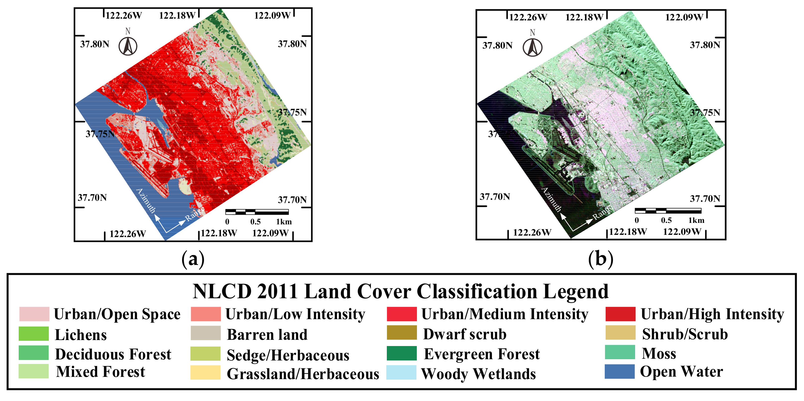
Figure 9.
Magnitudes of different criteria and histograms of selected patches: (a–c) the magnitudes of , , and respectively; and (d–f) the fitting histograms of the four patches.
Figure 9.
Magnitudes of different criteria and histograms of selected patches: (a–c) the magnitudes of , , and respectively; and (d–f) the fitting histograms of the four patches.

Figure 10.
Decomposition results of UAVSAR data: (a–d) surface, double-bounce, volume, and oriented dihedral scattering powers, respectively; (e) urban scattering power; and (f) color-coded decomposition result (blue, surface scattering; red, urban scattering; and green, volume scattering).
Figure 10.
Decomposition results of UAVSAR data: (a–d) surface, double-bounce, volume, and oriented dihedral scattering powers, respectively; (e) urban scattering power; and (f) color-coded decomposition result (blue, surface scattering; red, urban scattering; and green, volume scattering).

Figure 11.
Bar chart of decomposition power contribution of different land covers: (a) orthogonal buildings; (b) oriented buildings; (c) woods; and (d) ocean.
Figure 11.
Bar chart of decomposition power contribution of different land covers: (a) orthogonal buildings; (b) oriented buildings; (c) woods; and (d) ocean.
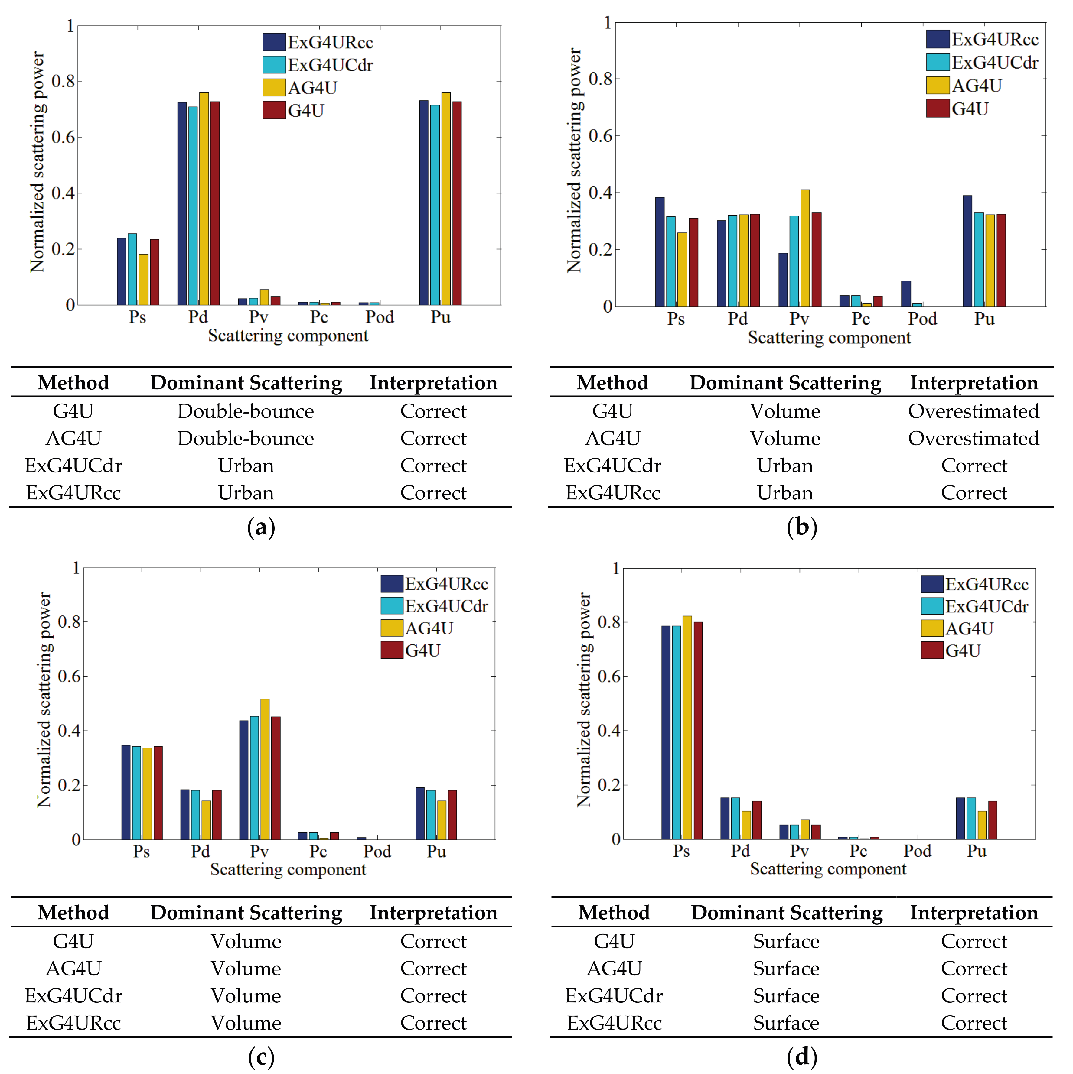
Figure 12.
Proposed decomposition results (blue-surface scattering, red-urban scattering, and green-volume scattering) and ground references for spaceborne data: (a,b) Radarsat-2 C-band data; and (c,d) ALOS PALSAR L-band data.
Figure 12.
Proposed decomposition results (blue-surface scattering, red-urban scattering, and green-volume scattering) and ground references for spaceborne data: (a,b) Radarsat-2 C-band data; and (c,d) ALOS PALSAR L-band data.

Figure 13.
Profile of decomposition scattering power: (a) Radarsat-2 C-band data; and (b) ALOS PALSAR L-band data.
Figure 13.
Profile of decomposition scattering power: (a) Radarsat-2 C-band data; and (b) ALOS PALSAR L-band data.


Table 1.
Averaged numerator of ratio of correlation coefficient for different wavebands.
| Band | Patch A | Patch B | Patch C | Patch D |
|---|---|---|---|---|
| C | 0.288 | 0.159 | 0.092 | 0.190 |
| L | 0.236 | 0.167 | 0.158 | 0.310 |
Table 2.
Averaged ratio of correlation coefficient for different wavebands.
| Band | Patch A | Patch B | Patch C | Patch D |
|---|---|---|---|---|
| C | 1.821 | 1.582 | 0.189 | 0.206 |
| L | 1.448 | 1.683 | 0.374 | 0.333 |
Table 3.
Normalized volume scattering power statistics for oriented urban areas.
| Band | G4U | AG4U | ExG4UCdr | ExG4URcc |
|---|---|---|---|---|
| C | 0.425 | 0.610 | 0.399 | 0.218 |
| L | 0.517 | 0.517 | 0.479 | 0.237 |
Table 4.
Normalized oriented dihedral scattering power statistics for oriented urban areas.
| Band | G4U | AG4U | ExG4UCdr | ExG4URcc |
|---|---|---|---|---|
| C | - | - | 0.009 | 0.101 |
| L | - | - | 0.006 | 0.129 |
Table 5.
Percentage of pixels with negative scattering powers for C-band data.
| Method | Ps < 0 or Pd < 0 (%) | Ps < 0 and Pd < 0 (%) |
|---|---|---|
| G4U | 11.0 | 26.1 |
| AG4U | 5.5 | 41.9 |
| ExG4UCdr | 10.5 | 20.2 |
| ExG4URcc | 4.8 | 10.7 |
Table 6.
Percentage of pixels with negative scattering powers for L-band data.
| Method | Ps < 0 or Pd < 0 (%) | Ps < 0 and Pd < 0 (%) |
|---|---|---|
| G4U | 15.3 | 6.4 |
| AG4U | 6.0 | 14.0 |
| ExG4UCdr | 4.0 | 3.3 |
| ExG4URcc | 2.7 | 3.3 |
Table 7.
Processed pixel statistics of artificial areas.
| Criterion | Pixel Count | Actual Pixel Count |
|---|---|---|
| 40,579 | 135,875 | |
| 44,802 | ||
| 82,705 |
© 2017 by the authors. Licensee MDPI, Basel, Switzerland. This article is an open access article distributed under the terms and conditions of the Creative Commons Attribution (CC BY) license (http://creativecommons.org/licenses/by/4.0/).
Share and Cite
MDPI and ACS Style
Quan, S.; Xiang, D.; Xiong, B.; Hu, C.; Kuang, G. A Hierarchical Extension of General Four-Component Scattering Power Decomposition. Remote Sens. 2017, 9, 856. https://doi.org/10.3390/rs9080856
AMA Style
Quan S, Xiang D, Xiong B, Hu C, Kuang G. A Hierarchical Extension of General Four-Component Scattering Power Decomposition. Remote Sensing. 2017; 9(8):856. https://doi.org/10.3390/rs9080856
Chicago/Turabian StyleQuan, Sinong, Deliang Xiang, Boli Xiong, Canbin Hu, and Gangyao Kuang. 2017. "A Hierarchical Extension of General Four-Component Scattering Power Decomposition" Remote Sensing 9, no. 8: 856. https://doi.org/10.3390/rs9080856
Note that from the first issue of 2016, this journal uses article numbers instead of page numbers. See further details here.