A Method to Improve High-Resolution Sea Ice Drift Retrievals in the Presence of Deformation Zones

1
The Alfred Wegener Institute, Helmholtz Centre for Polar and Marine Research, Bussestraße 24, 27570 Bremerhaven, Germany
2
Center for Integrated Remote Sensing and Forecasting for Arctic Operations, Arctic University of Norway, Sykehusvegen 21, 9019 Tromsø, Norway
*
Author to whom correspondence should be addressed.
Remote Sens. 2017, 9(7), 718; https://doi.org/10.3390/rs9070718
Submission received: 5 May 2017
/
Revised: 6 July 2017
/
Accepted: 9 July 2017
/
Published: 12 July 2017
(This article belongs to the Section Ocean Remote Sensing)
Abstract
:Retrievals of sea ice drift from synthetic aperture radar (SAR) images at high spatial resolution are valuable for understanding kinematic behavior and deformation processes of the ice at different spatial scales. Ice deformation causes temporal changes in patterns observed in sequences of SAR images; which makes it difficult to retrieve ice displacement with algorithms based on correlation and feature identification techniques. Here, we propose two extensions to a pattern matching algorithm, with the objective to improve the reliability of the retrieved sea ice drift field at spatial resolutions of a few hundred meters. Firstly, we extended a reliability assessment proposed in an earlier study, which is based on analyzing texture and correlation parameters of SAR image pairs, with the aim to reject unreliable pattern matches. The second step is specifically adapted to the presence of deformation features to avoid the erasing of discontinuities in the drift field. We suggest an adapted detection scheme that identifies linear deformation features (LDFs) in the drift vector field, and detects and replaces outliers after considering the presence of such LDFs in their neighborhood. We validate the improvement of our pattern matching algorithm by comparing the automatically retrieved drift to manually derived reference data for three SAR scenes acquired over different sea ice covered regions.
1. Introduction
The drift of sea ice can be observed from space by synthetic aperture radar (SAR), and quantified using drift detection algorithms. The requirements that the applied algorithm has to meet regarding resolution, reliability, and computing time varies with the type of application. If the drift information has to be provided in near real-time, the algorithm has to be fast, which means that only simple retrieval methods can be used. Such methods result in maps of ice drift with a comparatively coarse spatial resolution. Here, we focus on the retrieval of high-resolution sea ice drift information to document especially the small-scale kinematic behavior of sea ice and its deformation. The drift detection algorithm used in our work is based on pattern recognition to determine the displacement of recognizable sea ice structures in sequential SAR images [1]. We note that the application of the algorithm results in displacements of structures that can be identified in the ice cover. The drift is approximated from the straight line between the positions of a given structure derived from images 1 and 2, divided by the temporal difference between the acquisitions of both images. The true motion in this time interval is unknown. Our algorithm provides reliable drift and deformation information at a spatial resolution of 15 times the pixel size of the used SAR image. In our study, we used SAR images with pixel sizes between 50 and 150 m, which means that the spatial resolutions of the drift fields range between 750 m and 2.3 km. Typical spatial resolutions reported in other studies of sea ice drift derived from SAR imagery varied between 5 and 10 km [2,3].
An inhomogeneous drift of sea ice causes deformation processes such as a local opening in the ice cover or ice compression. The results of such processes are visible as, e.g., open water leads, ridges or rafting zones. Sea ice deformation changes the local ice thickness and triggers the production of new ice in open water leads. Thus, deformation is an important component of sea ice dynamics that affects the interaction between atmosphere, ocean, and ice. To detect patterns of sea ice deformation, which often appears localized as narrow structures in a sea ice cover [4,5], it is important to obtain spatially dense information about the ice drift, especially close to the zones of deformation. Here, a problem arises because patterns in the ice that are used for tracking ice displacements from SAR image pairs may change when deformation takes place between the acquisitions of the two SAR images. Resulting incorrect pattern matches of the drift detection algorithm may lead to incorrect drift vectors, which affects the magnitude of the sea ice deformation parameters calculated from the drift field. Therefore, the identification of incorrect drift vectors is important, and the implementation of procedures for detecting unreliable pattern matches and outliers as modules of an ice tracking algorithm leads to a higher reliability of the resulting drift and deformation retrievals.
For the present study, we extended the pattern matching algorithm that was introduced by Thomas et al. [6] and modified by Hollands and Dierking [1]. It is a cascaded multi-scale multi-resolution algorithm that combines a phase correlation (PC) and a normalized cross-correlation (NCC) technique to identify matching structures in sequential SAR images. The combination of PC and NCC is useful; the advantage of the latter is its higher robustness against image noise (speckle), whereas the PC is computationally efficient and more robust with respect to non-linear ice drift, such as ice floe rotation [7]. Pattern matching is performed such that the grid of the drift vector field is changed from coarse to dense spacing (“cascades”). At the same time, a resolution pyramid is built, starting with a resampled SAR image of relatively coarse pixel size and ending at the pixel size of the original image. Details of this processing are described in Thomas et al. [6] and Hollands and Dierking [1]. The size of the correlation window for pattern matching is determined by the balance between a robust correlation and the achievable spatial resolution of the drift field. As a result of this procedure, we obtain sea ice drift patterns on different spatial scales. Thereby, the need for initial drift information is avoided, and the stability of the algorithm is increased. The negative impact of artificial drift outliers is reduced by using a running box median filter. According to Thomas et al. [6], this method of outlier removal provides a simple and effective means of data regularization. However, it should be noted that the use of an averaging filter involves a loss of small-scale information due to smoothing of real discontinuities, and due to the loss of statistical independence between adjacent drift vectors. To avoid this disadvantage, an adaptive method for the detection of outliers that explicitly takes the existence of discontinuities into account, and a reliability assessment of the individual pattern matches, are both needed.
Hollands et al. [8] found that in algorithms based on pattern matching, the correlation coefficient alone is not sufficient to judge the reliability of a drift vector. Therefore, they introduced an index for reliability assessment, denoted as “confidence factor” (CFA), which combines different metrics that quantify particular image properties. Four parameters characterizing the image texture and two parameters related to the normalized cross-correlation are calculated: mean intensity gradient (MIG), mean gradient slope (MGS), variance-to-squared-mean-ratio (VMR), intensity threshold (IT), correlation coefficient (NCCC), and confidence interval of the correlation coefficient (NCCI). For these parameters, Hollands et al. [8] determined thresholds above which a pattern match and the corresponding drift vector are regarded unreliable. As the algorithm proceeds through the cascaded resolution pyramids, the CFA is increased by one every time a texture or correlation parameter exceeds the threshold. A high CFA hence indicates areas in which the retrieved drift vectors are less reliable.
Lavergne et al. [9] presented a concept to find outliers in a drift vector field by including the direct neighborhood of each drift vector. An outlier is detected when the deviation to the average of the adjacent vectors is above a predefined threshold. In this case, pattern matching using a maximum cross-correlation is repeated with adapted constraints for the corresponding search area.
In this paper, we focus on methods to determine unreliable pattern matches, and to detect and replace outliers in the sea ice drift retrieval, considering the presence of discontinuities in the drift vector field. To this end, we combine, modify, and extend the concepts of Hollands et al. [8] and Lavergne et al. [9], and add them to the drift detection algorithm implemented by Hollands and Dierking [1]. To avoid the replacement of a drift discontinuity by a smoothed velocity transition, we develop an adapted data regularization scheme that identifies linear deformation features (LDFs) in the drift field. To verify the improvement attributed to the implemented extensions, we calculate benchmarks derived from the differences between automatically derived drift vectors and manually determined reference data. Finally, we discuss the influence of sea ice deformation zones in a sea ice cover on the accuracy of drift detection algorithms.
2. Materials and Methods
2.1. Reliability Assessment
Hollands et al. [8] introduced the concept of the confidence factor (CFA) to assess the reliability of the retrieved drift vectors. The CFA is a combination of different parameters that reflect the structural characteristics of each image, which are determined by intensity texture, speckle, and single extreme high-intensity spots due to specular reflections from the ice surface. In addition, it includes the correlation between the two images from which ice displacements are calculated, and its confidence interval. We divide the CFA into two categories, i.e., image texture (texture_CFA) and correlation parameters (correlation_CFA). The total CFA is the sum of both. The texture_CFA consists of four parameters for characterizing the ice structure that were already applied by Hollands et al. [8] (Table 1). It is determined in each step of the drift algorithm (i.e., in each cascade and the particular step in the resolution pyramid) from the spatial variations of the backscattering intensities inside predefined areas (correlation windows) in images 1 and 2. Thereby homogeneous (texture free) areas such as ice shelves or zones of open water are identified and marked, for which pattern matching is not feasible. To evaluate the reliability based on the correlation (correlation_CFA), we modified the procedure described in Hollands et al. [8]. Here, both the PC and the NCC between the correlation windows in images 1 and 2 are quantified by the coefficient of the NCC-coefficient (denoted as NCCC) and the relative peak magnitude of the PC (denoted as RPM), which is given by:
Here, is the mean of the correlation matrix (which contains the results for the different spatial lags between the two correlation windows).
In comparison to Hollands et al. [8], our design of the correlation_CFA results in a stronger influence of the correlation measures on the total CFA. The purpose of the correlation_CFA is not only to detect highly unreliable pattern matches on the basis of the correlation parameters, but also to establish a rank order of reliable drift candidates. To determine the threshold ranges for the correlation_CFA (shown in Table 1), we minimized retrieval errors derived in comparison to reference data (see Section 2.3) by varying the ranges of the NCCC and RPM. Additionally, we adjusted values such that both subcategories of the CFA contribute an almost equivalent amount to the total CFA. The correlation_CFA is in most cases obtained from the NCC. Only if the PC provides a reliable correlation (CFA_PC < 4), while the NCC does not (CFA_NCC = 4), the former is used to determine the drift vector and the correlation_CFA. This case occurs in particular in ice regions with non-linear drift patterns (e.g., rotation of ice floes). As shown in Figure 1, the CFA serves to flag areas/matches revealing a low reliability based on the combination of texture properties and correlation parameters.
In many cases, the results of the PC and NCC reveal more than one reliable correlation peak. If a drift vector based on the highest correlation peak appears as an outlier in comparison to its adjacent vectors an alternative drift candidate of the preceding correlation procedure iteratively replaces it (Figure 1b, box 1 under “Replacement”). In the first step, only drift vectors with the same CFA are potential candidates to replace the outlier. If these vectors still appear as outliers, alternative matches with a lower CFA are accepted. If no candidate fits into its neighborhood, or no other correlation peak is reliable (CFA_NCC = 4 and CFA_PC = 4), the median of adjacent vectors is used for replacement. Whether all or only certain vectors from the neighborhood are used for calculating the median is decided based on the result of the procedure for detecting discontinuities described in Section 2.2. We found that more than 50% of the outliers are replaced by an alternative drift candidate retrieved from the correlation data, and in the other cases, the outliers had to be replaced by the median determined from the adjacent drift vectors, as explained below. This item will be further addressed in the discussion below.
2.2. Detection of LDFs and Outliers
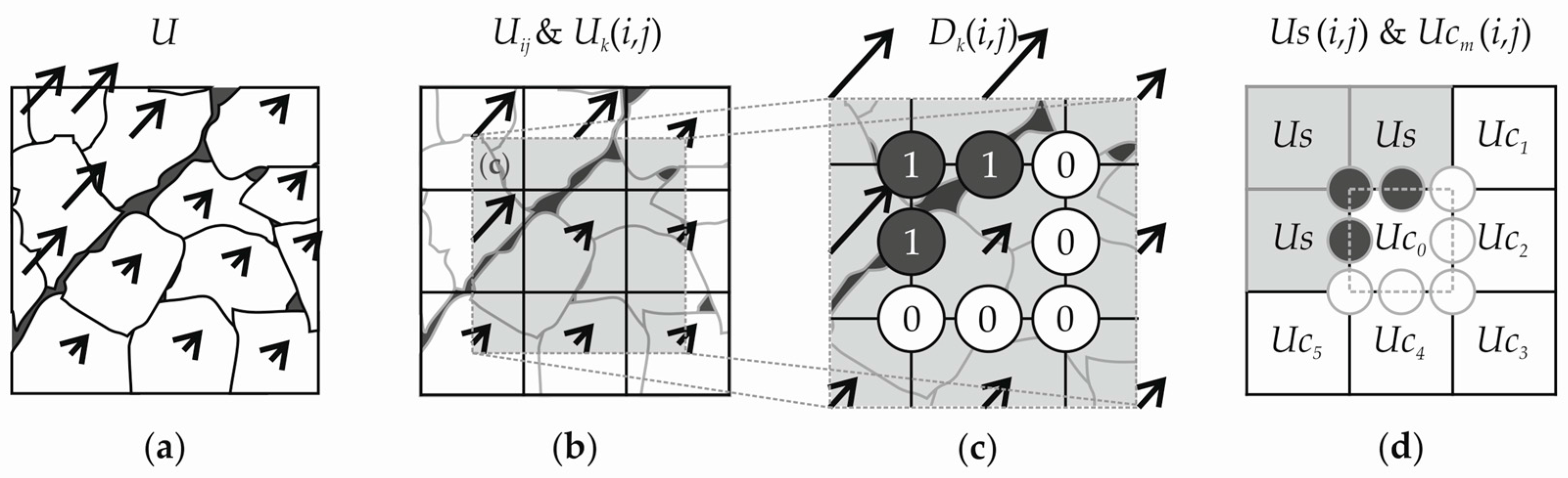
The detection of drift vectors that deviate significantly in magnitude and/or direction from their neighborhood (in this text denoted as “outliers”) represents a very important part of our modified drift retrieval algorithm. One has to consider that in areas of active deformation processes, discontinuities occur in the ice drift field that require special procedures for the detection and replacement of outliers. The aim of our new method is to adapt the application of averaging filters to the presence of discontinuities, and thus preserve drift variations caused by real sea ice deformation. To achieve this, the algorithm considers the presence of sea ice deformation features (denoted as linear deformation features, LDF, in the following), which appear as localized linear or quasi-linear structures [10] when detecting drift discontinuities in running windows over 3 × 3 grid cells. If an LDF is detected, the algorithm divides each window into two segments: vectors that reveal relative small deviations to the central vector (denoted as “connected” vectors, Uc), and vectors with larger deviations that are separated from the central vector by the LDF (denoted as “separated” vectors, US). The subsequent detection of an outlier is then carried out by calculating statistics (Section 2.2.3) only on the connected vectors, to preserve the drift discontinuities.
2.2.1. Spatial Distribution of Discontinuities and Identification of LDFs
As mentioned above, distinct discontinuities in the drift vector field are determined in a window covering 3 × 3 grid cells (Figure 2). The absolute velocity gradient between the central drift vector Uij and its adjacent vectors Uk in all eight discrete directions is calculated and stored in an 8-element velocity gradient vector G:
where k is linked to the positions of the adjacent drift vectors:
and I and J are the dimensions of the retrieved drift vector field, u and v are the components of the drift vector U, and Δs is the distance between the positions of two drift vectors. With Δx and Δy being the grid spacing of the vector field in x- and y-direction, we obtain, e.g., Δsi−1,j = Δx and Δsi−1,j−1 = (Δx2 + Δy2)1/2. To differentiate between a continuous gradient and a discontinuity, a threshold is defined, which is determined in each cascade and resolution step as follows: Except for the outermost margin of a gridded drift field of size (I, J) we determine the gradients Gk(i,j), i = 1…I − 1, j = 1…J − 1, k = 1…4 in 3 × 3 windows for all grid cells in the image. For each window position, only the three grid cells above the center point and the grid cell to its left are considered to avoid double counts. Note that Gk(i,j) is calculated from the differences between center and adjacent grid cells, hence overlap zones between single windows reveal different gradients for each window position except for one cell, if the overlap ≥4 cells. The probability density function (PDF) is evaluated from the gradients over the entire drift field. An exponential function is then fitted to the PDF. In the next step, the value is calculated at which the cumulative distribution function (CDF) of the exponential fit is 0.9545. This point determines the twofold standard deviation of all velocity gradient values. As demonstrated in Figure 3, gradients above this threshold are considered as a discontinuity. The motivation and implications of this detection method are clarified in the discussion below. The identified discontinuities are stored in the binary decision vector Dk for each position i,j:
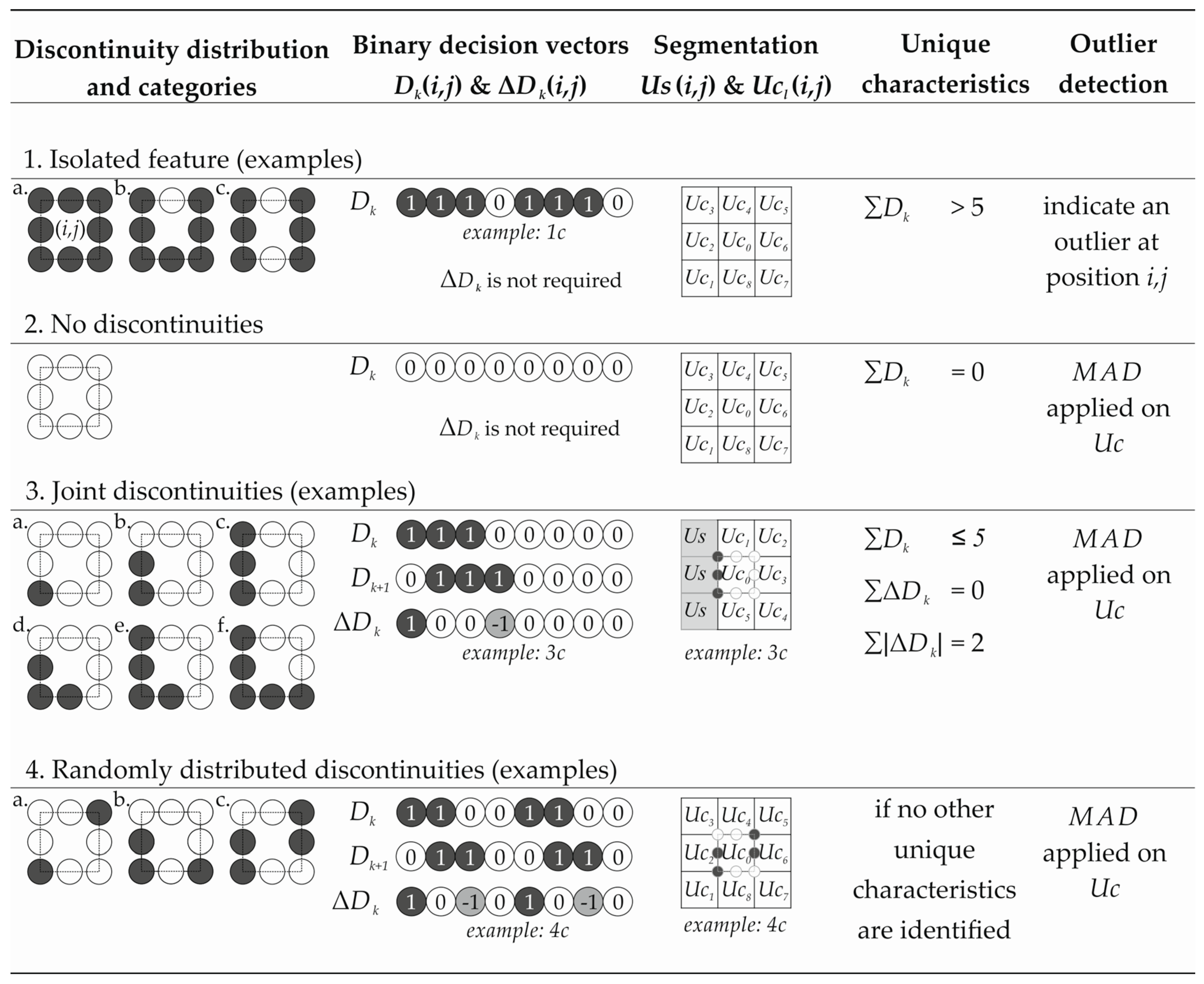
In the next step, the position i,j is categorized considering the spatial distribution of the identified discontinuities: isolated feature (1), no discontinuities (2), joint discontinuities (3), and randomly distributed discontinuities (4). The typical characteristics of these types are shown in Figure 4. Note that the eight grid cells around the center of the window represent gradients (categorized by their magnitude, according to Equation (3)). To determine the prevalent category, we defined unique characteristic of Dk and the “ring differences” ΔDk (Equations (3) and (4)) for each category (Figure 4, row 4).
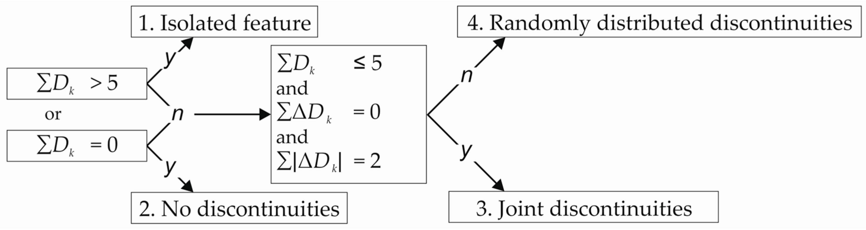
In Figure 5, we show the decision scheme that is used to distinguish between the four categories. Because of the invariance of the applied method to a transposition or a rotation of the elements in the 3 × 3 window, all 28 constellations are efficiently taken into account regarding the computational effort.
2.2.2. Segmentation by LDFs
Category 1 (isolated feature) indicates an outlier at position i,j and no further detection step is required. Category 2 (no discontinuities) is trivial. Category 3 (joint discontinuities) represents an LDF; thus the 3 × 3 window is divided into the two segments: “separated” and “connected” drift vectors (see Figure 2 and Figure 4). Category 4 (randomly distributed discontinuities) is not assignable to an LDF; consequently, all vectors are considered as connected.
2.2.3. Adapted Outlier Detection
To detect outliers in category 2, 3 and 4, the median absolute deviation (MAD) is applied on the segment of connected drift vectors Ucl in each window of 3 × 3 grid cells at the position i,j:
where b (=1.4826) is a constant linked to the assumption that data are normally distributed. The index l = 1…L refers to the L-connected drift vectors Ucl. The MAD is a robust statistic in the presence of outliers, and not sensitive to the sample size [11,12]. An outlier in the center of the 3 × 3 window is detected if M > 2∙MAD, and replaced as described in Figure 1b and Section 2.1. If M ≤ 2∙MAD, the central drift vector matches into its neighborhood and remains unchanged.
2.3. Validation
To validate the applied methods, we generated a reference data set by visually tracking stable sea ice structures that can be identified in the sequential SAR images. For further investigations, we selected the structures such that they occur in different distances from the drift field discontinuities (see Section 3). The absolute and the relative difference between a reference and the corresponding automatically retrieved drift vector are denoted as retrieval errors Eabs and Erel, respectively:
We calculated five benchmark values representing the algorithm accuracy: B1 is the mean over all individual errors, B2 the root mean square of Ex, and B3 the mean angular error:
where x can be either abs or rel, and n is the number of reference vectors. B4 and B5 are the number of the relative errors Erel greater than 10% (B4) and 50% (B5). A relative error of 10% represents a reasonable metric used in many practical applications [13], and a relative error higher than 50% is considered a complete failure of the algorithm.
We verified the improvement of the retrieved sea ice drift by implementing multiple versions (A1–A5) of our drift detection algorithm (see Table 2). The first version (A1) is the original cascaded multi-scale multi-resolution pattern matching algorithm without a reliability assessment (CFA) and any data regularization. The second version (A2) represents the algorithm discussed in Hollands and Dierking [1], with no intrinsic use of the reliability assessment or explicit outlier detection, but with application of a running box median filter. In the third version (A3), the algorithm is extended by the intrinsic use of the reliability assessment to decide whether conditions for a successful pattern matching are met. The fourth version (A4) builds on A3, and performs the presented outlier detection using the MAD on each window of 3 × 3 grid cells without preceding window segmentation. The final version (A5) includes the latter.
2.4. Calculation of Sea Ice Deformation Parameters
To determine whether a dependency of the algorithm accuracy to sea ice deformation exists, we derived the deformation parameters directly from the retrieved sea ice drift field. The parameters are usually calculated from the invariants of the strain rate tensor comprising the partial derivatives of the drift field [14]:
Following Lindsay and Stern [15], we computed the partial derivatives by an approximation of the line integral around the boundary of each grid cell (e.g., ∂u/∂x):
where A is the area of the grid cell calculated using Gauss’s area formula, and the other partial derivatives are determined analogously.
2.5. Test Sites, SAR and Reference Data
Each test site comprised two sequential SAR images, which are geocoded and calibrated using the commercial software SAR-Scape. The SAR image pairs were acquired over two regions in the Weddell Sea (Ronne Polynya and central southern Weddell Sea), and north of Fram Strait in the Arctic. The coordinates of the overlapping areas between the image pairs are listed in Table 3. The selected test sites represented different ice conditions. Also, the sensor configurations (frequency, spatial resolution, imaging modes) and the time gaps between the acquisitions of the two SAR images are different. The reference data used for validating our results comprise about 100 manually derived drift vectors per test site.
3. Results
3.1. Drift Retrievals and Algorithm Accuracy
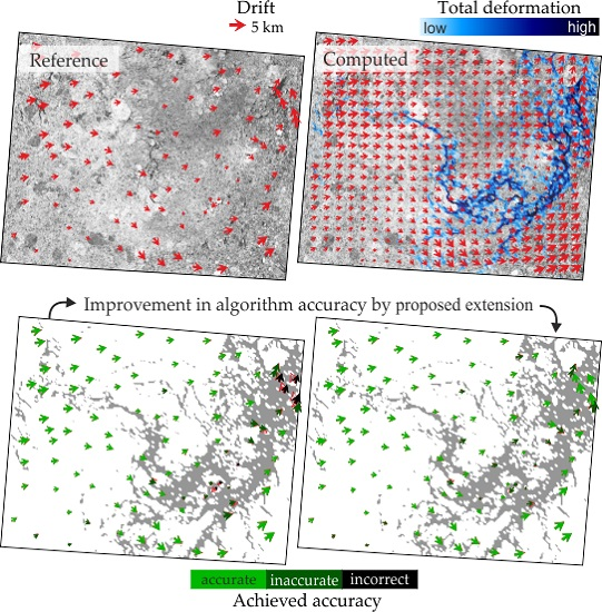
The drift detection algorithm used in our work provides high-resolution sea ice drift retrievals with spacing between drift vectors between 750–2250 m (see Table 3). Table 4 lists parameter of sea ice kinematic that quantify differences in sea ice kinematics between the three test sites. The kinematic parameters are directly derived from the drift vectors obtained with the algorithm version A5 (Section 2.4) As an example, Figure 6 shows retrieved drift vectors in comparison to the reference vectors, and the automatically determined total deformation for the SAR scene acquired in the Weddell Sea. The comparison of the retrieved drift (A3 and A5) and the reference drift (Figure 6c,d) reveals the improvement of the accuracy of the former in areas of larger deformation rates when the algorithm version A5 is applied.
To display the change in algorithm accuracy for all three test sites and all five algorithm versions, we provide the results for the benchmarks introduced in Section 2.3 in Table 5. The values demonstrate the highest consistency between reference and automatically retrieved sea ice drift vectors when the extended algorithm A5 was applied. Except for one case, all benchmarks indicate higher algorithm accuracy for each extension of the algorithm from versions A1 to A5. The exception occurs in the scene acquired over the Arctic Ocean, for which the mean angular error B3 increases between retrievals obtained from version A2 and A3. A closer examination revealed that the total error was dominated by the individual error of a single drift vector. Here, the reliability assessment replaced a “short” vector indicating a low drift velocity with a vector with a wrong orientation. This example demonstrates that the reliability check may deteriorate the final result in rare cases.
The high values of benchmark B4 obtained for the Weddell Sea are due to the short time gap between acquisitions of images 1 and 2, which results in smaller absolute displacements of sea ice structures. However, the number indicating a complete failure of the algorithm (B5) is much lower and decreased considerably through the different implementation steps.
In general, the improvement attributed to the reliability assessment (A3) is—with the one exception discussed above—significant in all drift fields for the three test sites shown in Table 5. In combination with the adapted outlier detection (A5), the algorithm provides highly accurate drift retrievals. The mean relative error (B1rel) of all three scenes is lower than 10%, and the number indicating a complete failure of the algorithm (B5) decreases to 0.
We found the most distinct improvement for the Weddell Sea scene, which exhibited the highest sea ice deformation rates ( in Table 4). This observation supports the assumption that an erroneous retrieval of a drift vector can be mainly attributed to the existence of discontinuities in the drift field. In Figure 7, we quantify the dependence between the relative error Erel and the distance to a severe deformation. The total deformation per acquisition time gap Δt (Equations (12)–(14)) is derived using the output of algorithm version A5, since it represents the most reliable sea ice drift field. We considered a total deformation greater than 0.2 per time interval Δt as severe, and used the corresponding locations as reference for calculating the minimum distance to the adjacent drift vectors, for which the relative errors obtained from versions A1 to A5 of the retrieval algorithm could be determined relative to a reference vector. Figure 7 shows results for A1, A3, and A5. If the distance to a severe deformation is larger than two times the grid spacing (2ΔS), a sufficiently low error is achieved. Inaccurate drift vectors (Erel > 10%) are primarily observed particularly close (distance < 2ΔS) to a severe deformation. Highly inaccurate vectors (Erel > 50%) only occur in A1 and A3.
3.2. Computational Efficiency
Table 6 shows the computing time of the applied algorithm in seconds, and the resulting number of retrieved drift vectors for all three scenes and algorithm versions A1 and A5. It should be noted that the algorithm was not optimized regarding the computational efficiency, and that the grid resolution (spacing between drift vectors) is much higher compared to most other results of SAR based drift detection algorithms discussed in the literature. The intention here is to demonstrate the computational effort of the introduced methods by comparing algorithm versions A1 and A5. The variables that affect the computing time are the number of performed cascade and pyramid steps, the number of retrieved drift vectors, and the complexity of the sea ice drift patterns. The number of algorithm steps was fixed to 12 (four cascade and three pyramid steps), and the grid spacing of the drift vector field was set to 15 times the SAR resolution. The investigation area size varied from 14,000 km2 to 100,000 km2. We observe the highest computing time per 100 vectors for the test site from the Weddell Sea, which exhibited the most complex sea ice kinematics. The inclusion of the algorithm extensions proposed here even decreased the computing time for this scene by a factor of 0.8. An explanation for this is the drift regularization in preceding algorithm steps, which led to a more efficient correlation procedure in subsequent steps. In the other two scenes, the computing time was increased by a factor of 1.15 (Arctic Ocean) and 1.25 (Ronne Polynya).
4. Discussion
The achieved increase of the retrieval accuracy justifies the application of the two extensions to the ice drift detection algorithm that we suggested in this study. The additional computing effort is appropriate. The degree of improvement depends on the ice conditions and kinematics. These parameters determine the presence of discontinuities in the ice drift field that indicate the formation of a deformation structure. However, sensor configurations and acquisition time gaps also have to be considered, as the former influence the image texture, and the latter affect the correlation.
The modified CFA allows a better reliability assessment of the individual pattern matches. In comparison to the CFA introduced by Hollands et al. [8], we included both correlation methods (NCC and PC). In addition, we apply partitioned thresholds that allow a more precise assessment based on the correlation parameters (see Table 1). One issue in this context is that the thresholds for the texture_CFA determined by Hollands et al. [8], and also used in our study, are based on C-band SAR data. Thus, a future task is to test and—where appropriate—adapt thresholds and ranges of the texture_CFA for different radar bands.
In addition to the original algorithm described by Hollands and Dierking [1], we use the results of both correlation methods (PC and NCC) for the retrieval of a drift vector. To this end, we implemented a data regularization scheme that replaces vector outliers primarily by alternative matches from the correlation procedure (i.e., secondary peaks of the correlation functions). As demonstrated in Figure 8, the drift retrieval includes more alternative drift vectors derived from pattern matches than vectors calculated as median from adjacent vectors. Because no general averaging filter is applied, and the implemented identification of LDFs preserves drift discontinuities, smoothing effects are minimized. These points are important in order to investigate the small-scale kinematic behavior of sea ice and its deformation processes.
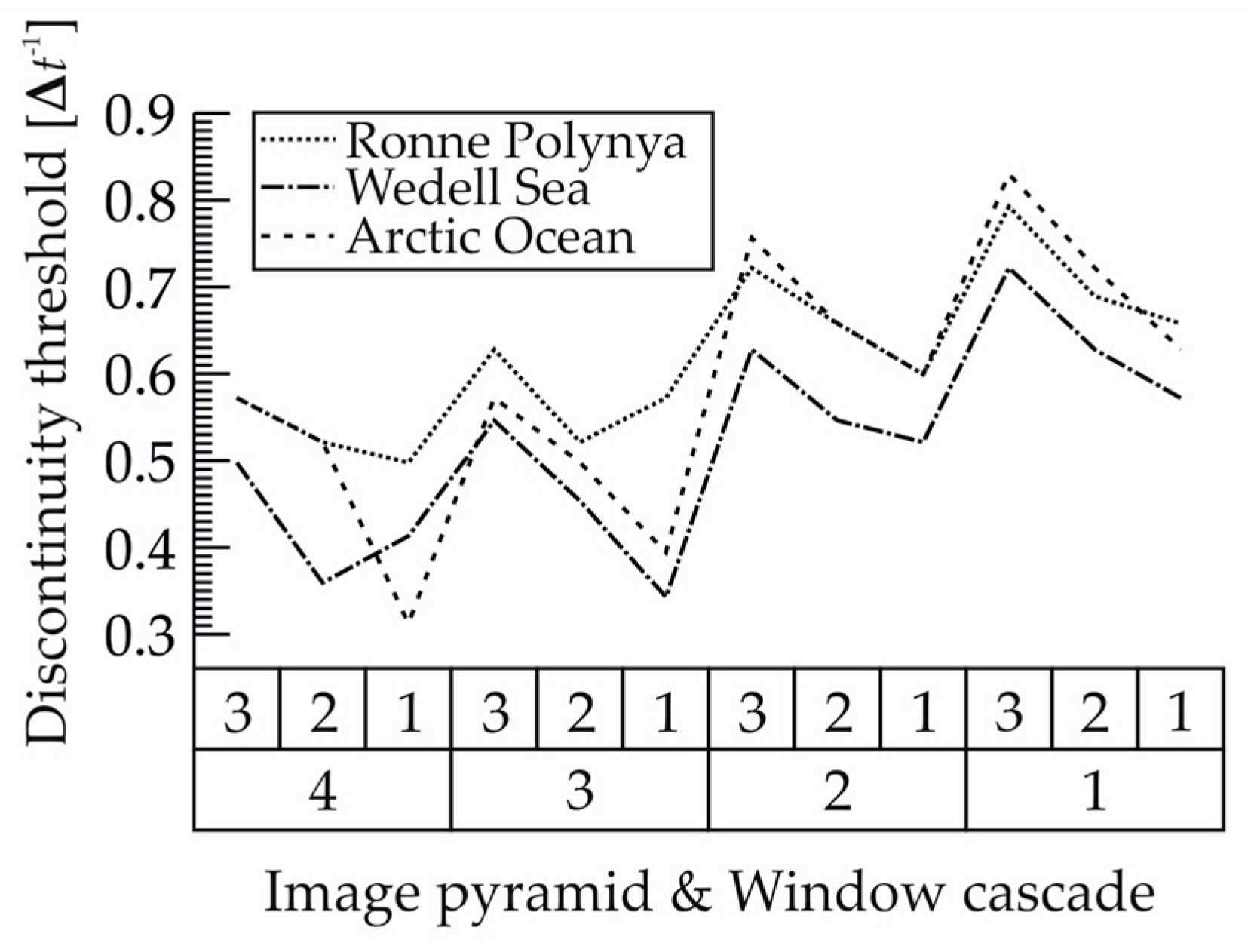
Compared to other published methods that identified drift outliers e.g., [9,15,16], we implemented a method that automatically calculates thresholds for identifying outliers in the drift field. The detection of an outlier using the MAD is based on the relative deviation of a vector compared to its neighbors (see Equations (5) and (6)). The threshold for detecting a discontinuity is determined from the velocity gradients retrieved from the entire vector field in the overlap area between images 1 and 2 (Figure 3). However, since the absolute value of the threshold in terms of the velocity gradient that is obtained as suggested depends on the variability of the drift vector field, it does not present a “global” threshold for detecting a discontinuity. To solve this problem, more data sets need to be analyzed to implement a method that considers the magnitude and spatial variability of the ice drift. It has also to be taken into account that the threshold depends on spatial and temporal scales. Figure 9 shows the variation of the automatically adapted discontinuity threshold at the different spatial scales of the three resolution pyramids as they progress through the four cascades. Results are shown for the three test sites Table 4, which differ in their acquisition time gaps and their ice kinematics.
An analysis of sea ice deformation regarding spatial and temporal scales has revealed a strong heterogeneous and intermittent character of the deformation e.g., [17,18,19]. Thus, deformation becomes more and more localized at smaller scales, with severe deformation occupying a smaller fraction of the total area [10]. Our cascaded algorithm automatically retrieves drift on an Eulerian grid at different spatial scales. Hence, it is possible to analyze the dependence of the deformation on different spatial scales and derive information about the mechanical behavior of the ice at those scales. The high accuracy of our algorithm, and especially the improvement in accuracy when deformation zones are present, allows reliable scaling analysis of the derived sea ice deformation. As part of future investigations, we plan to extend recently published results towards smaller spatial scales. We regard the algorithm presented here as a useful tool for those investigations.
5. Conclusions
The present work introduced two extensions to algorithms for sea ice drift detection based on pattern matching. One was related to the check of the reliability of the individual pattern matches, and the other to the detection and replacement of vector outliers in the vicinity of discontinuities in the drift field. The motivation was to improve the accuracy of the retrieved drift vector field, and to preserve the discontinuities in the drift field, since they represent zones of sea ice deformation. We showed that erroneous drift vectors appear more frequently close to active deformation zones. If outliers have to be replaced, an alternative reliable drift vector obtained from the correlation matrix can be found in more than 50% of all cases; hence the use of median values can be avoided. We demonstrated the applicability of our algorithm on data sets from three different ice-covered ocean regions representing different SAR acquisition parameters and ice conditions. The conducted benchmark test indicates that the extended reliability assessment and advanced outlier detection result in higher algorithm accuracy and higher reliability of the resulting drift vector retrievals and the derived deformation parameters. The drift and deformation products that are the output of our algorithm are the basis for further studies towards understanding the kinematic and mechanic behavior of sea ice and its deformation processes over a wide range of spatial scales.
Acknowledgments
Jakob Griebel was funded by the Helmholtz Alliance ‘Remote Sensing and Earth System Dynamics’, WP-C5, which we gratefully acknowledge. The Envisat ASAR images were provided by ESA, Cat-1 project C1P.5024. TerraSAR-X data were obtained from project OCE2173. We would like to thank Thomas Busche, who acted as PI of this project, for his help and support. We used Copernicus Sentinel-1 data acquired over an area north of Fram Strait in January 2015.
Author Contributions
Jakob Griebel developed and implemented the extension modules to the sea ice drift retrieval algorithm of the Earth Observing Systems Group at AWI. Wolfgang Dierking contributed to the development of the concept and the design of each module. Both authors wrote the text.
Conflicts of Interest
The authors declare no conflict of interest.
References
- Hollands, T.; Dierking, W. Performance of a multiscale correlation algorithm for the estimation of sea-ice drift from SAR images: Initial results. Ann. Glaciol. 2011, 52, 311–317. [Google Scholar] [CrossRef]
- Holt, B.; Rothrock, D.A.; Kwok, R. Determination of sea ice motion from satellite images. In Microwave Remote Sensing of Sea Ice; American Geophysical Union: Washington, DC, USA, 1992; pp. 343–354. [Google Scholar]
- Pedersen, L.T.; Saldo, R.; Fenger-Nielsen, R. Sentinel-1 results: Sea ice operational monitoring. In Proceedings of the 2015 IEEE International Geoscience and Remote Sensing Symposium (IGARSS), Milan, Italy, 26–31 July 2015; pp. 2828–2831. [Google Scholar]
- Dierking, W.; Dall, J. Sea-Ice Deformation State from Synthetic Aperture Radar Imagery—Part I: Comparison of C- and L-Band and Different Polarization. IEEE Trans. Geosci. Remote Sens. 2007, 45, 3610–3622. [Google Scholar] [CrossRef]
- Tin, T.; Jeffries, M.O. Morphology of deformed first-year sea ice features in the Southern Ocean. Cold Reg. Sci. Technol. 2003, 36, 141–163. [Google Scholar] [CrossRef]
- Thomas, M.; Geiger, C.A.; Kambhamettu, C. High resolution (400 m) motion characterization of sea ice using ERS-1 SAR imagery. Cold Reg. Sci. Technol. 2008, 52, 207–223. [Google Scholar] [CrossRef]
- Reddy, B.S.; Chatterji, B.N. An FFT-based technique for translation, rotation, and scale-invariant image registration. IEEE Trans. Image Process. 1996, 5, 1266–1271. [Google Scholar] [CrossRef] [PubMed]
- Hollands, T.; Linow, S.; Dierking, W. Reliability Measures for Sea Ice Motion Retrieval from Synthetic Aperture Radar Images. IEEE J. Sel. Top. Appl. Earth Obs. Remote Sens. 2015, 8, 67–75. [Google Scholar] [CrossRef]
- Lavergne, T.; Eastwood, S.; Teffah, Z.; Schyberg, H.; Breivik, L.-A. Sea ice motion from low-resolution satellite sensors: An alternative method and its validation in the Arctic. J. Geophys. Res. 2010, 115, C10032. [Google Scholar] [CrossRef]
- Marsan, D.; Stern, H.; Lindsay, R.; Weiss, J. Scale Dependence and Localization of the Deformation of Arctic Sea Ice. Phys. Rev. Lett. 2004, 93, 178501. [Google Scholar] [CrossRef] [PubMed]
- Huber, P.J.; Ronchetti, E. Robust Statistics; John Wiley & Sons: Hoboken, NJ, USA, 2009. [Google Scholar]
- Leys, C.; Ley, C.; Klein, O.; Bernard, P.; Licata, L. Detecting outliers: Do not use standard deviation around the mean, use absolute deviation around the median. J. Exp. Soc. Psychol. 2013, 49, 764–766. [Google Scholar] [CrossRef]
- Thomas, M.V. Analysis of Large Magnitude Discontinuous Non-Rigid Motion. Ph.D. Thesis, University of Delaware Newark, Newark, DE, USA, 2008. [Google Scholar]
- Thorndike, A.S.; Colony, R. Sea ice motion in response to geostrophic winds. J. Geophys. Res. 1982, 87, 5845. [Google Scholar] [CrossRef]
- Lindsay, R.W.; Stern, H.L. The RADARSAT Geophysical Processor System: Quality of Sea Ice Trajectory and Deformation Estimates. J. Atmos. Ocean. Technol. 2003, 20, 1333–1347. [Google Scholar] [CrossRef]
- Komarov, A.S.; Barber, D.G. Sea Ice Motion Tracking From Sequential Dual-Polarization RADARSAT-2 Images. IEEE Trans. Geosci. Remote Sens. 2014, 52, 121–136. [Google Scholar] [CrossRef]
- Muckenhuber, S.; Korosov, A.A.; Sandven, S. Open-source feature-tracking algorithm for sea ice drift retrieval from Sentinel-1 SAR imagery. Cryosphere 2016, 10, 913–925. [Google Scholar] [CrossRef]
- Hutchings, J.K.; Roberts, A.; Geiger, C.A.; Richter-Menge, J. Spatial and temporal characterization of sea-ice deformation. Ann. Glaciol. 2011, 52, 360–368. [Google Scholar] [CrossRef]
- Rampal, P.; Weiss, J.; Marsan, D.; Lindsay, R.; Stern, H. Scaling properties of sea ice deformation from buoy dispersion analysis. J. Geophys. Res. 2008, 113, C03002. [Google Scholar] [CrossRef]
Figure 1.
Flow diagram of the correlation procedure (a) and the outlier detection/handling; (b) CW1,2—Correlation window pair for performing the PC (phase correlation), NCC (normalized cross correlation), and the various CFA parameters, CFA—confidence factor, T—texture. See Section 2.1 and Section 2.2 for further explanation.
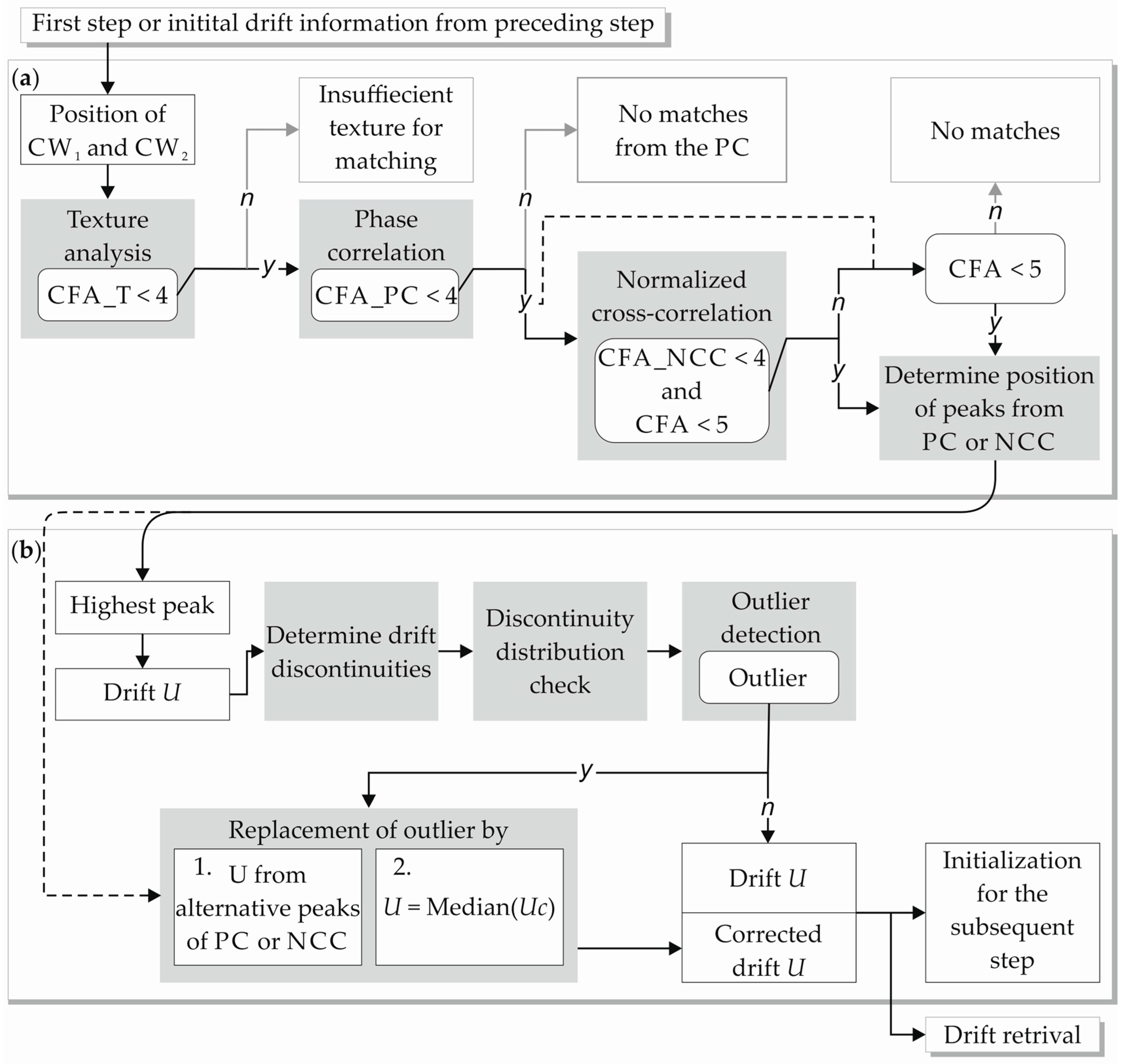
Figure 2.
Schematic sea ice drift of a shear zone: (a) Drift of individual floes; (b) discretized drift; (c) spatial distribution of discontinuities; and (d) segmentation of the window of 3 × 3 grid cells. Indices i, j, k are explained in the text following Equation (2).
Figure 2.
Schematic sea ice drift of a shear zone: (a) Drift of individual floes; (b) discretized drift; (c) spatial distribution of discontinuities; and (d) segmentation of the window of 3 × 3 grid cells. Indices i, j, k are explained in the text following Equation (2).

Figure 3.
Probability density function (PDF) of the absolute velocity gradient Gijk and the exponential fit. Absolute gradients higher than two standard deviations (2σ) are considered as discontinuities.
Figure 3.
Probability density function (PDF) of the absolute velocity gradient Gijk and the exponential fit. Absolute gradients higher than two standard deviations (2σ) are considered as discontinuities.

Figure 4.
Examples of the spatial distribution of discontinuities at position i,j for all categories, the binary decision vector Dk and the calculation of the “ring difference” ΔDk. The white circles indicate small gradients (≤2σ), the black ones indicate large gradients considered as discontinuities (>2σ) (see Figure 2). The third column shows the segmentation of the 3 × 3 grid cell window required for the outlier detection and median calculation. The fourth column presents the unique characteristics for the identification of the respective category. In the fifth column, the method to detect an outlier in the corresponding category is listed. Category 1 (isolated feature) directly indicates an outlier at position i,j.

Figure 5.
Decision schema of the spatial distribution of discontinuities (category 1, 2, 3, and 4), and the queries of the unique characteristics introduced in Figure 4.
Figure 5.
Decision schema of the spatial distribution of discontinuities (category 1, 2, 3, and 4), and the queries of the unique characteristics introduced in Figure 4.

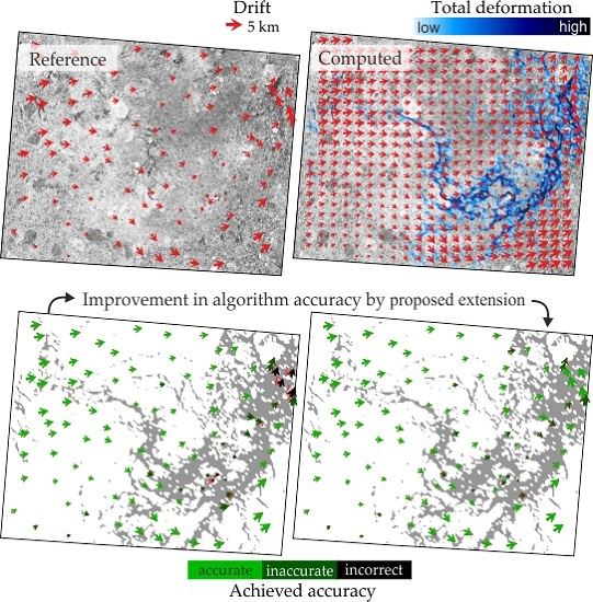
Figure 6.
TerraSAR-X scene acquired in the Weddell Sea. (a) Manually derived reference drift and (b) automatically retrieved drift using algorithm A5. The upper right image (b) includes the total deformation. The lower images show the difference between reference vectors and the drift retrieved using A3 (c) and A5 (d) (grey background: total deformation greater than 0.2 per time interval Δt).
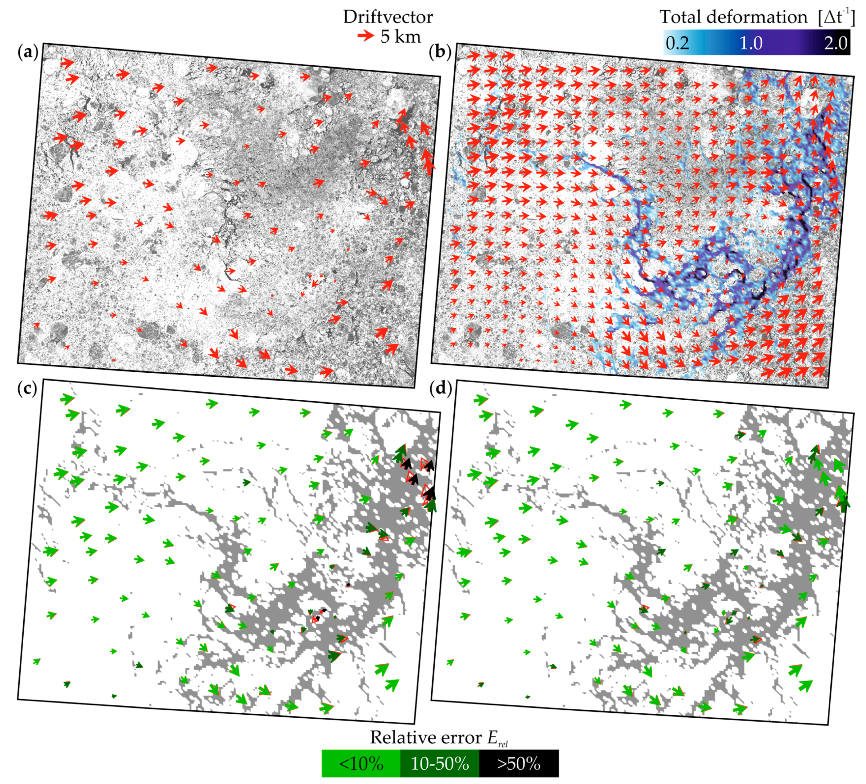
Figure 7.
Dependence of the relative error (Erel, logarithmic) on the distance to a severe deformation (εtotal > 0.2).
Figure 7.
Dependence of the relative error (Erel, logarithmic) on the distance to a severe deformation (εtotal > 0.2).
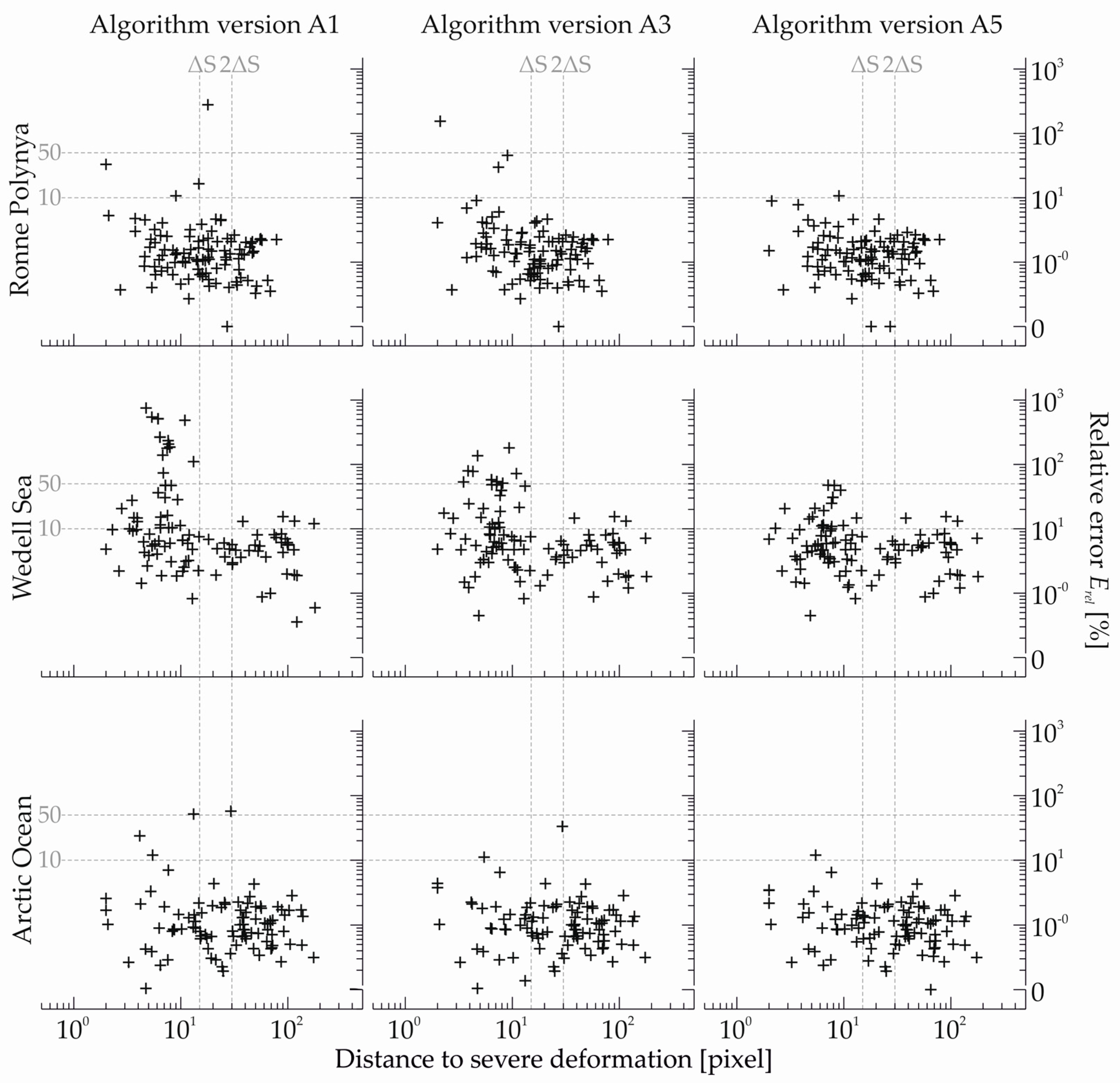
Figure 8.
The mean percentage of all detected outliers, and the used replacement method of these outliers. —mean total deformation rate, Δt—acquisition time gap, ΔS—grid spacing.
Figure 8.
The mean percentage of all detected outliers, and the used replacement method of these outliers. —mean total deformation rate, Δt—acquisition time gap, ΔS—grid spacing.
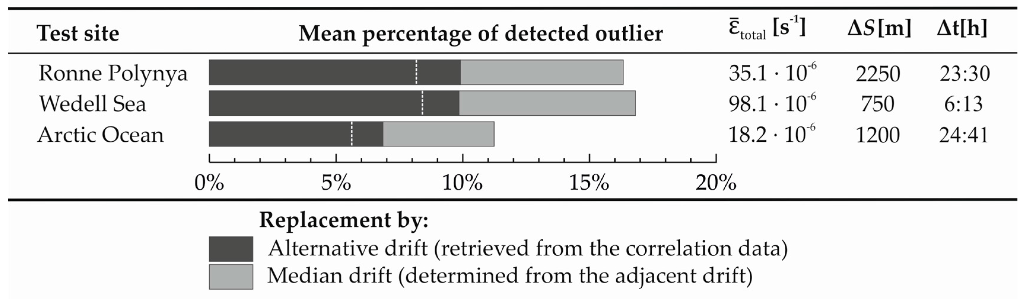
Figure 9.
Variation of the threshold to identify discontinuities (2σ of the velocity gradient distribution, see Section 2.2.1) at the different spatial scales of the algorithm steps for all test sites.
Figure 9.
Variation of the threshold to identify discontinuities (2σ of the velocity gradient distribution, see Section 2.2.1) at the different spatial scales of the algorithm steps for all test sites.

Table 1.
Thresholds and ranges for determination of the confidence factor.
| Confidence Factor | Abbreviations | Threshold/Range | Value |
|---|---|---|---|
| Texture_CFA (see [8]) | CFA_T | 0–4 | |
| Variance-to-squared-mean-ratio | VMR | <0.5 | +1 |
| Mean intensity gradient | MIT | <1.7 | +1 |
| Mean gradient slope | MGS | <0.35 | +1 |
| Intensity threshold | IT | >−3 dB | +1 |
| Correlation_CFA (obtained from NCC or PC) | CFA_NCC or CFA_PC | 0–4 | |
| NCC (coefficient and confidence interval) | NCCC | <0.1 | =4 |
| 0.1–0.2 | =3 | ||
| 0.2–0.4 | =2 | ||
| 0.4–0.8 | =1 | ||
| >0.8 | =0 | ||
| NCCI | >0.2 | =4 | |
| PC (Relative peak magnitude) | RPM | <1.58 | =4 |
| 1.58–2.51 | =3 | ||
| 2.51–3.98 | =2 | ||
| 3.98–6.31 | =1 | ||
| >6.31 | =0 | ||
| Confidence factor | CFA | 0–8 |
Table 2.
The applied methods of the five algorithm versions
| Methods | Algorithm Version | ||||
|---|---|---|---|---|---|
| A1 | A2 | A3 | A4 | A5 | |
| Median filter | X | X | |||
| Intrinsic use of the reliability assessment | X | X | X | ||
| Outlier detection using MAD | X | X | |||
| Preceding window segmentation by a identified LDF | X | ||||
Table 3.
Test sites and SAR data description.
| Region | Ronne Polynya | Weddell Sea | Arctic Ocean |
|---|---|---|---|
| Extent of the overlap (N/S) | 74°S/77°S | 73.4°S/75°S | 85°N/80.5°N |
| Extent of the overlap (W/E) | 64°W/49°W | 39°W/33.5°W | 17°E/48.5°E |
| Overlapping area | 60,000 km2 | 14,000 km2 | 100,000 km2 |
| Satellite | Envisat ASAR | TerraSAR-X | Sentinel-1 |
| Reprojection | Polar Stereographic | Polar Stereographic | Polar Stereographic |
| Band & mode | C, Wide Swath | X, ScanSAR | C, Extra Wide Swath |
| Used resolution | 150 m | 50 m | 80 m |
| Date | 22/23 February 2008 | 14/15 February 2014 | 1/2 January 2015 |
| Season | Summer | Summer | Winter |
| Acquisition time gap (Δt) | 23:30 h | 6:13 h | 24:41 h |
| Drift grid spacing (ΔS) | 2250 m | 750 m | 1200 m |
Table 4.
Parameter of sea ice kinematic.
| Region | Ronne Polynya | Weddell Sea | Arctic Ocean |
|---|---|---|---|
| Mean absolute drift [ms−1] | 0.094 | 0.036 | 0.231 |
| Mean total deformation rate [s−1] | 4.007 × 10⁻⁶ | 10.616 × 10⁻⁶ | 1.981 × 10⁻⁶ |
| Mean divergence rate [s−1] | −0.191 × 10⁻⁶ | −0.113 × 10⁻⁶ | −0.351 × 10⁻⁶ |
| Mean shear rate [s−1] | 3.287 × 10⁻⁶ | 9.003 × 10⁻⁶ | 1.725 × 10⁻⁶ |
Table 5.
Results of the algorithm accuracy benchmarks (B1–B5) for the algorithm versions (A1–A5).
| Test Site | Algorithm Accuracy Benchmarks | |||||||||
|---|---|---|---|---|---|---|---|---|---|---|
| B1abs | B1rel | B2abs | B2rel | B3 | B4 | B5 | ||||
| [pixel] | [m] | [%] | [pixel | m] | [%] | [°] | ||||
| Ronne Polynya Envisat ASAR 22/23 February 2008 | A1 | 3.89 | 584 | 4.8 | 24.10 | 3616 | 27.9 | 2.40 | 4 | 1 |
| A2 | 2.21 | 331 | 4.1 | 5.08 | 763 | 15.1 | 1.31 | 4 | 1 | |
| A3 | 1.84 | 276 | 3.8 | 4.15 | 622 | 14.4 | 1.17 | 3 | 1 | |
| A4 | 1.19 | 179 | 1.8 | 1.54 | 232 | 2.5 | 0.65 | 1 | 0 | |
| A5 | 1.16 | 174 | 1.7 | 1.48 | 222 | 2.4 | 0.60 | 1 | 0 | |
| Weddell Sea TerraSAR-X 14/15 February 2014 | A1 | 30.35 | 1518 | 48.0 | 90.54 | 4527 | 124.3 | 20.39 | 37 | 15 |
| A2 | 13.54 | 677 | 20.2 | 28.03 | 1401 | 36.5 | 13.84 | 37 | 14 | |
| A3 | 8.60 | 430 | 14.9 | 15.71 | 786 | 32.3 | 7.58 | 29 | 11 | |
| A4 | 5.05 | 253 | 11.4 | 7.76 | 388 | 31.7 | 5.55 | 25 | 3 | |
| A5 | 4.13 | 207 | 7.7 | 5.64 | 282 | 11.5 | 3.08 | 21 | 0 | |
| Arctic Ocean Sentinel-1 01/02 January 2015 | A1 | 6.97 | 558 | 2.6 | 25.05 | 2004 | 8.1 | 1.08 | 4 | 2 |
| A2 | 5.64 | 451 | 2.0 | 23.87 | 1909 | 6.4 | 0.62 | 2 | 1 | |
| A3 | 4.20 | 337 | 1.7 | 12.10 | 966 | 3.9 | 0.74 | 2 | 0 | |
| A4 | 3.44 | 276 | 1.5 | 5.52 | 441 | 2.2 | 0.58 | 1 | 0 | |
| A5 | 3.08 | 246 | 1.3 | 4.04 | 323 | 2.0 | 0.54 | 1 | 0 | |
Table 6.
Computing time of algorithm version A1 and A5, and the number of drift vectors for the given SAR scenes.
Table 6.
Computing time of algorithm version A1 and A5, and the number of drift vectors for the given SAR scenes.
| Test Site | Number Drift Vectors | Computing Time | |||
|---|---|---|---|---|---|
| Total [s] | per 100 Vectors [s] | ||||
| A1 | A5 | A1 | A5 | ||
| Ronne Polynya | 14,000 | 170 | 210 | 1.2 | 1.5 |
| Weddell Sea | 29,000 | 580 | 460 | 2.0 | 1.6 |
| Arctic Ocean | 77,000 | 1000 | 1200 | 1.3 | 1.5 |
© 2017 by the authors. Licensee MDPI, Basel, Switzerland. This article is an open access article distributed under the terms and conditions of the Creative Commons Attribution (CC BY) license (http://creativecommons.org/licenses/by/4.0/).
Share and Cite
MDPI and ACS Style
Griebel, J.; Dierking, W. A Method to Improve High-Resolution Sea Ice Drift Retrievals in the Presence of Deformation Zones. Remote Sens. 2017, 9, 718. https://doi.org/10.3390/rs9070718
AMA Style
Griebel J, Dierking W. A Method to Improve High-Resolution Sea Ice Drift Retrievals in the Presence of Deformation Zones. Remote Sensing. 2017; 9(7):718. https://doi.org/10.3390/rs9070718
Chicago/Turabian StyleGriebel, Jakob, and Wolfgang Dierking. 2017. "A Method to Improve High-Resolution Sea Ice Drift Retrievals in the Presence of Deformation Zones" Remote Sensing 9, no. 7: 718. https://doi.org/10.3390/rs9070718
Note that from the first issue of 2016, this journal uses article numbers instead of page numbers. See further details here.