
3D Imaging of Greenhouse Plants with an Inexpensive Binocular Stereo Vision System

1
College of Information Science and Technology, Donghua University, Shanghai 201620, China
2
College of Electronics and Information Engineering, Tongji University, Shanghai 201804, China
*
Author to whom correspondence should be addressed.
Remote Sens. 2017, 9(5), 508; https://doi.org/10.3390/rs9050508
Submission received: 18 March 2017
/
Revised: 16 May 2017
/
Accepted: 17 May 2017
/
Published: 21 May 2017
Abstract
:Nowadays, 3D imaging of plants not only contributes to monitoring and managing plant growth, but is also becoming an essential part of high-throughput plant phenotyping. In this paper, an inexpensive (less than 70 USD) and portable platform with binocular stereo vision is established, which can be controlled by a laptop. In the stereo matching step, an efficient cost calculating measure—AD-Census—is integrated with the adaptive support-weight (ASW) approach to improve the ASW’s performance on real plant images. In the quantitative assessment, our stereo algorithm reaches an average error rate of 6.63% on the Middlebury datasets, which is lower than the error rates of the original ASW approach and several other popular algorithms. The imaging experiments using the proposed stereo system are carried out in three different environments including an indoor lab, an open field with grass, and a multi-span glass greenhouse. Six types of greenhouse plants are used in experiments; half of them are ornamentals and the others are greenhouse crops. The imaging accuracy of the proposed method at different baseline settings is investigated, and the results show that the optimal length of the baseline (distance between the two cameras of the stereo system) is around 80 mm for reaching a good trade-off between the depth accuracy and the mismatch rate for a plant that is placed within 1 m of the cameras. Error analysis from both theoretical and experimental sides show that for an object that is approximately 800 mm away from the stereo platform, the measured depth error of a single point is no higher than 5 mm, which is tolerable considering the dimensions of greenhouse plants. By applying disparity refinement, the proposed methodology generates dense and accurate point clouds of crops in different environments including an indoor lab, an outdoor field, and a greenhouse. Our approach also shows invariance against changing illumination in a real greenhouse, as well as the capability of recovering 3D surfaces of highlighted leaf regions. The method not only works on a binocular stereo system, but is also potentially applicable to a SFM-MVS (structure-from-motion and multiple-view stereo) system or any multi-view imaging system that uses stereo matching.

1. Introduction
Greenhouse cultivation, which is a kind of highly integrated facility agriculture, is becoming increasingly important in raising the efficiency of agricultural production and solving the world’s food shortage. Despite its significance, modern greenhouse cultivation still faces challenges to increase output and meanwhile reduce energy consumption. For this purpose, an economic, efficient, and intelligent greenhouse environment control method is needed to guarantee a temperate environment for each plant during its whole growth period, and to accomplish high yields and economic benefits. As a branch of remote sensing, 3D imaging uses the most direct manner to fully present the continuous growth of greenhouse plants via imaged shapes and spatial structures. The technique not only helps to monitor and manage plant growth, but also provides visual cues that optimize the intelligent greenhouse environment control system, which controls the greenhouse actuators such as roof windows, shading nets, ventilations, and so on.
Plant phenotyping is the quantitative analysis of the structure and function of plants. With rapid advances in DNA sequencing technologies, plant phenotyping is becoming a bottleneck in cultivating crops with higher yields [1]. Currently, most solutions for plant phenotyping are way too expensive for practical use. Even though some of them can be affordable, many are designed for their own specific tasks, resulting in low generality in application. The fast developing 3D sensing technology is arousing attentions from both academics and industry; it is now an essential tool to obtain information for plant phenotyping. Low-cost and efficient 3D imaging methods facilitate the development of high-throughput plant phenotyping, and the obtained 3D features of plants are also helpful in variety selection and the breeding process in modern agriculture. In some cases, phenotypic features of crops also imply economic meaning. 3D sensors can automatically recognize good samples in fruit and vegetable sorting. A 3D imaging system is also able to classify better shaped ornamentals that are later sold at a higher price.
Since the early 1990s, researchers have been using imaging tools to monitor and analyze plant growth, and methods based on 2D images are widely investigated for the first time for agricultural purposes such as identifying plants and weeds [2,3,4], leaf recognition [5,6,7], fruit detection [8], and advanced warning of plant diseases and pests [9]. Scharr et al. made a recent survey [10] of state-of-the-art 2D methods for leaf segmentation in plant phenotyping, and evaluated the results of the IPK 3D histograms [11], Nottingham SLIC superpixels [12], MSU Chamfer matching [13,14], and Wageningen watersheds segmentation on Arabidopsis (Arabidopsis thaliana (L.) Heynh.) and tobacco plants (Nicotiana tabacum L.). Fernández et al. [15] designed an automatic system that combines RGB and 2D multispectral imagery for discriminating grapevine crop organs such as leaves, branches, and fruits in field tests. Li et al. [16] developed a method to identify blueberry fruits in several different growth stages in 2D images acquired under natural scenes. 2D techniques are popular for ease of use and flexible equipment requirements. Nevertheless, they have several disadvantages: (1) environmental light changes can easily interfere with the imaging process and cause image degradation; (2) 2D techniques usually have restrictions on relative positions and directions between the device and the plant; and (3) an ordinary image loses the depth information about the scene, hence it is hard to fully characterize the spatial distributions of a sample plant. In order to faithfully reveal how a plant grows, it is necessary to capture its complicated 3D structure, especially in the canopy area. 3D imaging is essentially a kind of non-destructive remote sensing methodology. 3D sensors generally operate by projecting electromagnetic energy onto an object and then record the reflected energy (active form) [17], or by directly acquiring transmitted electromagnetic energy from scenes (passive form) to depict spatial objects and surfaces. Prevailing 3D imaging methods can be classified into several categories such as Time-of-Flight, laser scanning, structured light systems, light-field imaging, and stereo vision.
A Time-of-Flight (ToF) camera measures the time of the light that travels between the sensor and an object, and then estimates the distance between them to plot the depth map. In order to detect vegetation in the field of view, Nguyen et al. used a ToF camera and a CMOS camera to construct a multi-sensor imaging platform for a mobile robot [18]. Alenya et al. [19] used a ToF camera that attached to a robot to automatically measure plants, and they obtained satisfactory 3D point clouds of leaves. Fernández et al. [20] proposed a multisensory system including a ToF camera that provides fast acquisition of depth maps for localization of fruits on crops.
3D laser scanning uses the Lidar to project laser beams onto the surface, and uses triangulation to measure the reflected laser beams for reconstructing a dense 3D point cloud. Although commercial 3D laser scanners have very high accuracy, the high price greatly limits their application. Garrido et al. [21] used several 2D Lidars to form overlapped point clouds for 3D maize plant reconstruction. Seidel et al. [22] used a terrestrial Lidar to estimate the above-ground biomass of some potted juvenile trees. Xu et al. [23] used a laser scanner to image trees; they first reconstructed a tree skeleton containing main branches from scanned data, and then added 3D leaves to visualize a realistic tree. Dassot et al. [24] used terrestrial laser scanner to estimate wood solid volume in a forest in a non-destructive way, and the estimated value is close to the labor-intensive destructive measurements.
Structured light systems first project structured light patterns onto the object, and then capture the reflected pattern to compute the 3D geometry of the object surface. Dornbusch et al. used structured light technique to scan barley plant for graphic 3D reconstruction [25]. Li et al. used structured light systems to scan spatial–temporal point cloud data of growing plants, and successfully detected growth events such as budding and bifurcation [26].
Recently, emerging commercial 3D imaging sensors such as Kinect and light-field cameras have attracted attention from plant phenotyping community due to their low cost and high efficiency. Paulus et al. [27] compared 3D imaging results of a Kinect with results from a laser scanning system, and carried out phenotyping of beetroot and wheat. Chene et al. [28] used a Kinect sensor to conduct phenotyping experiments on a rosebush, and obtained perfect top-view depth maps. Li et al. [29] adopted Kinect for side-view imaging of two varieties of tomato plants in consecutive growth periods; vivid 3D visualization of tomato plants was realized after analyzing the digitized tomato organ samples. Yamamoto et al. [30] constructed a Kinect-based system for 3D measurement of a community of strawberries cultivated on a 1-meter-long bench in greenhouse. Schima et al. [31] applied the Lytro LF, an innovative low-cost light-field camera to monitor plant growth dynamics and plant traits, showing that this device could be a tool for on-site remote sensing. Phytotyping 4D [32], a light-field camera system was built by Apelt et al. for accurately measuring the morphological and growth-related features of plants.
Current 3D imaging methods still have several shortcomings when applied to crops or plants. First, the equipment is usually costly; second, some methods are subject to strict limitations on the ambient environment, whereas a greenhouse usually has a complex environment. Finally, it is hard to strike a balance between efficiency and accuracy. For example, some laser scanners need hours to complete a thorough scan, while commercial ToF cameras work in real time with very limited resolution. As a popular research direction in machine vision and remote sensing, stereo vision has advantages such as low cost and convenience; therefore, it may be a better choice for on-site 3D plant imaging. Stereo vision is a passive 3D imaging method that synthesizes object images from different views to reconstruct 3D surfaces. Biskup et al. [33] designed a stereo system that consists of two digital single lens reflex (DSLR) cameras to study shape deformation of leaves in a period of time. Teng et al. [34] first used multi-view stereo method to recover point clouds of leaves, and then implemented a 2D/3D joint graph-cut algorithm to segment leaves from canopy. Hu et al. [35] applied structure-from-motion (SFM) method and the multiple-view stereo (MVS) to generate dense point cloud of experimental plants from images, showing comparable accuracy with laser scanned result. Duan et al. [36] presented a similar workflow that contains SFM and MVS to characterize early plant vigor in wheat genotypes.
The imaging procedure of a typical stereo vision system consists of four steps—(i) camera calibration, (ii) stereo rectification, (iii) stereo matching, and (iv) 3D point cloud reconstruction. Stereo matching is the central part of a binocular/multi-view stereo vision system because the stereo correspondence search determines the quality of the point cloud or the depth image obtained. Common stereo matching algorithms comprise two categories: energy-based stereo matching algorithms [37,38] and filter-based algorithms [39,40]. In recent years, we have witnessed the filter-based stereo matching algorithms taking a qualitative leap in accuracy due to their remarkable edge-aware ability in imaging areas with abrupt depth changes. The adaptive support-weight approach (ASW) [39] is a powerful local filtering algorithm that not only can be perceived with bilateral filtering, but also can be explained by Gestalt psychology. The main idea of the ASW is to adjust the support weights of the pixels in a given window using color similarity and geometric proximity to reduce the ambiguity in matching [41]. In the original ASW framework, the truncated absolute differences (TAD) measure is used to calculate the raw matching cost of ASW. Despite its fast calculation, TAD can easily be affected by problems in real environments such as radiometric distortion and low-texture areas. The greenhouse usually has complex illumination because of the shadows cast by greenhouse structures and occlusions between plants. Plant leaves have similar green colors in the same canopy, resulting in ambiguous color feature and homogeneous textures. To address these challenges, we first built an effective and low-cost stereo vision system, and then incorporated the AD-Census cost measure [42] with the framework of ASW to improve the disparity map. The main objectives of this article include:
- (i)
- To build a highly feasible stereo platform that does not place harsh limitations on hardware and imaged objects. We established an inexpensive (less than 70 USD) and portable binocular stereo vision platform that can be controlled by a laptop. The platform is suitable for 3D imaging of many kinds of plants in different environments such as an indoor lab, open field, and greenhouse.
- (ii)
- To design an effective stereo matching algorithm that not only works on a binocular stereo system, but is also potentially applicable to a SFM-MVS system or any multi-view imaging systems. Improvements in the ASW stereo matching framework are made by replacing the TAD measure with AD-Census measure. The proposed algorithm shows superior results in comparison with the original ASW and several popular energy-based stereo matching algorithms.
- (iii)
- To perform error analysis of the stereo platform from both theoretical and experimental sides. Detailed investigation of the accuracy of the proposed platform under different parametric configurations (e.g., baseline) is provided. For an object that is about 800 mm away from our stereo platform, the measured depth error of a single point is no higher than 5 mm.
- (iv)
- To prove the effectiveness of the proposed methodology on 3D plant imaging by testing with real greenhouse crops. The proposed methodology generates satisfactory colored point clouds of greenhouse crops in different environments with disparity refinement. It also shows invariance against changing illumination, as well as a capability of recovering 3D surfaces of highlighted leaf regions.
2. Materials
2.1. Stereo Vision Platform
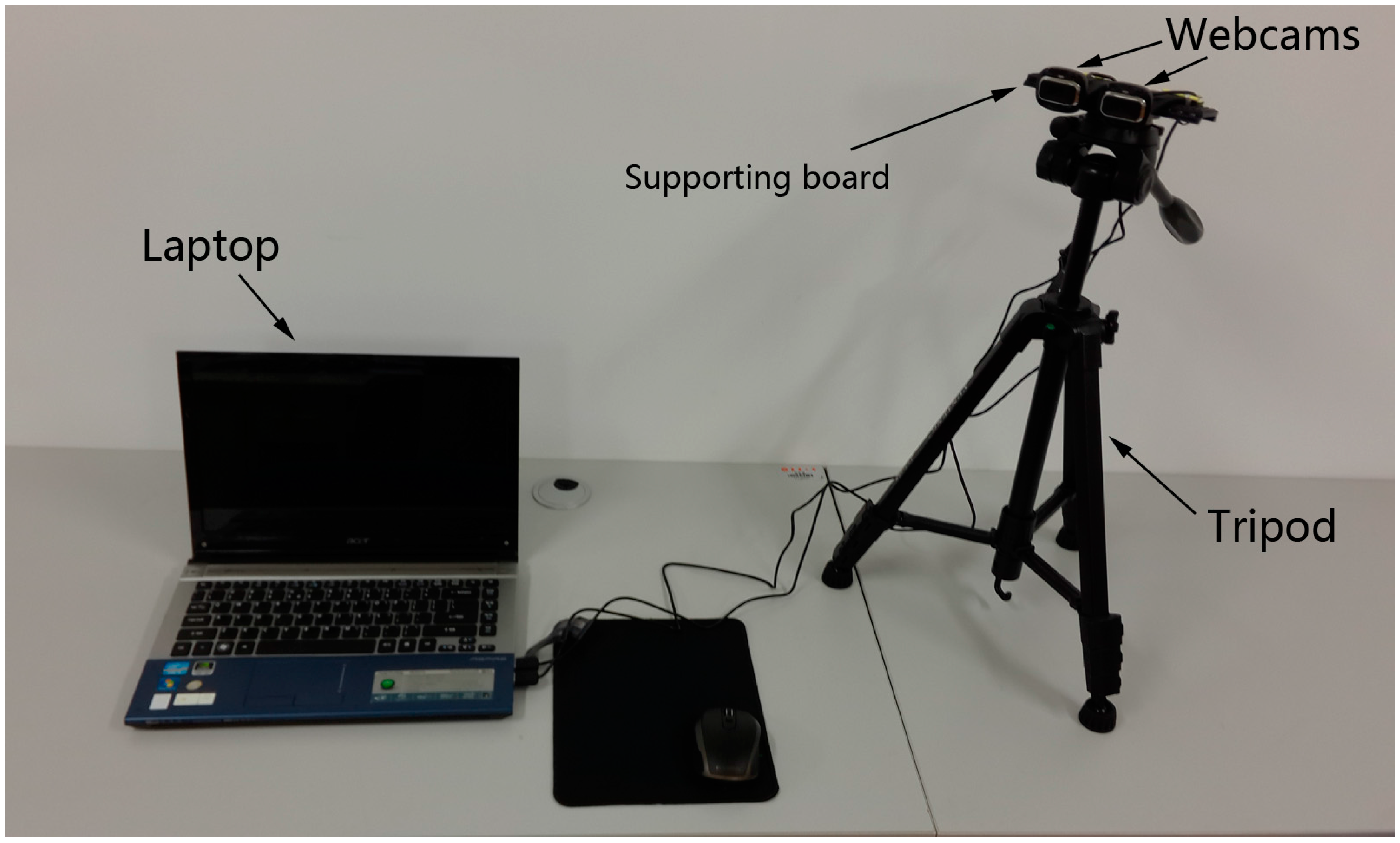
The proposed stereo vision platform consists of two high-definition webcams (HD-3000 series, Microsoft, Redmond, WA, USA). The camera incorporates a CMOS sensor supporting 720p HD video recording. The two cameras are placed onto a supporting board (LP-01, Fotomate, Jiangmen City, China) with a scale line, and the whole part is then mounted on a tripod (VCT-668RM, Yunteng Photographic Equipment Factory, Zhongshang City, China). The supporting board allows the distance (i.e., baseline) between the two cameras to be flexibly adjusted within a range from 40 mm to 110 mm. The processing unit is a laptop (4830T series, Acer, New Taipei City, Taiwan) with 4GB RAM and an Intel Core i5-2410M CPU. The structure of the system is shown in Figure 1. The price of the portable stereo vision platform without the laptop is less than 70 USD, much cheaper than any other 3D imaging devices or systems. The software environment includes VS2010 (Microsoft, Redmond, WA, USA) with an OpenCV library (Itseez, San Francisco, CA, USA), VS2013 (Microsoft, Redmond, WA, USA) with a PCL library (pointclouds.org), as well as MATLAB (MathWorks, Natick, MA, USA), and are all operated in Windows 10.
2.2. Sample Plants and Environments
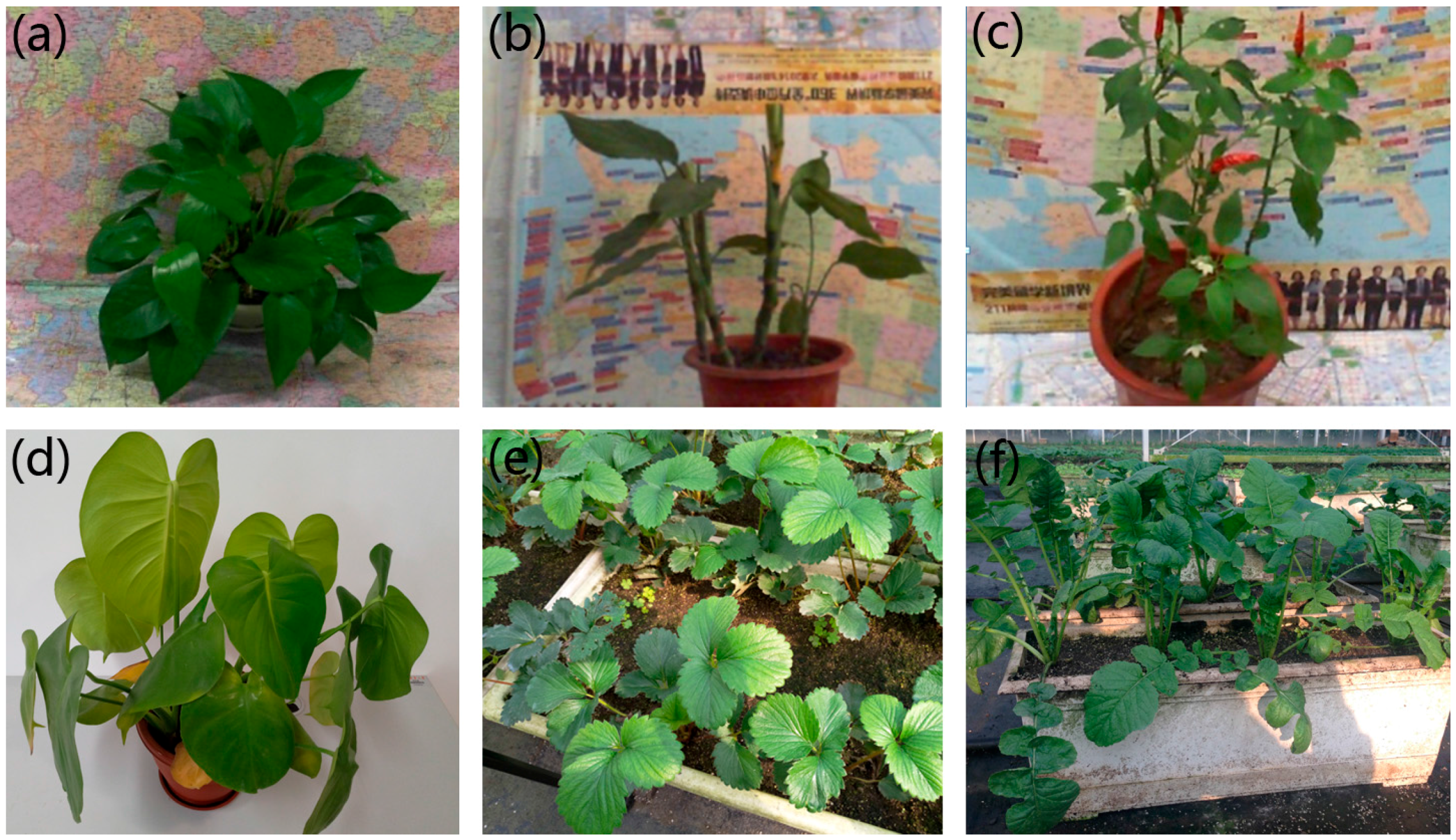
Six types of greenhouse plants are adopted as experiment subjects in this paper, including Epipremnum aureum (Linden & André) G.S. Bunting, Aglaonema modestum Schott ex Engl., pepper (Capsicum annuum L.), Monstera deliciosa L., cultivated strawberry (Fragaria × ananassa Duchesne), and turnip (Raphanus sativus L.), half of which are greenhouse ornamentals and the other half are greenhouse crops. Images of the six types of plants are exhibited in Figure 2. Epipremnum aureum, Aglaonema modestum, and pepper plants were used in 3D imaging experiments in the lab environment. A potted Monstera deliciosa sample was used in 3D imaging experiments in an open field. The strawberry and turnip crops were used for experiments in a real greenhouse.
The imaging experiments using the proposed stereo system were carried out in three different environments: an indoor lab (Donghua University, Shanghai, China), an open field with grass (Donghua University, Shanghai), and a multi-span glass greenhouse (Tongji University, Shanghai) under fully automated control. Images of the three environments are given in Figure 3. A hygrothermograph was used to record the temperature and relative humidity of each environment. During the experimentations, the average temperature of the indoor lab was 25.0 °C, and the relative humidity was 41%. The measured temperature and the relative humidity of the open field were 24.0 °C and 30% in the experiment, respectively. A four-day experiment on strawberry crops and turnip crops was conducted in the greenhouse. In order to test the proposed method’s robustness against the illumination changes, our stereo system operated in both sunny weather and overcast weather. The average temperature and the relative humidity in the greenhouse for strawberry plants were 22.5 °C and 57%, respectively, in the sunny day; and 20.5 °C and 58%, respectively, in overcast weather. The average temperature and the relative humidity in the greenhouse for turnip crops were 22.0 °C and 57%, respectively, when it was sunny, and 21.0 °C and 59%, respectively, in overcast weather.
3. Methodology
3.1. Framework
Binocular stereo vision is an important branch of machine vision and it is a technique aiming at inferring depth information of a scene via two cameras. In a standard stereo camera model, the two image planes are co-planar and are vertically aligned as shown in Figure 4. As we can see, is called baseline, which specifies the translation between the two projection centers. is the focal length of the two cameras. stands for the disparity, i.e., the pixel difference between the coordinates of two corresponding points in the left image and in the right image. In principle, the technique is able to recover the X, Y, and Z information of an object P by calculating the disparity of the corresponding pixels between two images taken from different viewpoints.
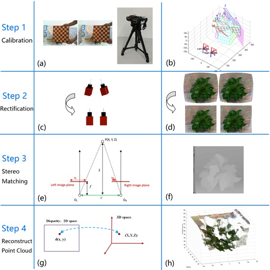
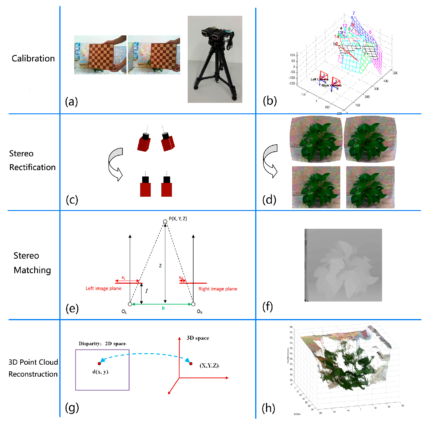
The imaging of a typical binocular stereo vision system consists of four steps: (i) camera calibration, (ii) stereo rectification, (iii) stereo matching, and (iv) 3D point cloud reconstruction. The first step computes camera parameters. The second step aligns epipolar lines in the left and right views, and reduces the 2D correspondence searching to 1D. The stereo matching is the key step, which finds pixel-wise correspondences between two images to generate a disparity map. The final step recovers 3D information from the disparity map by using triangulation and camera parameters. The four steps are displayed in Figure 5.
3.2. Calibration
Cameras need to be calibrated for two reasons: (a) calculating intrinsic parameters (focal length , principle point coordinates and distortion coefficient) and extrinsic parameters (camera rotation and translation with respect to the origin of the 3D world), and (b) correcting the lens distortion. We adopted a calibration toolbox for Matlab [43] that uses Zhang’s calibration method [44] to calibrate the cameras. This approach uses a pattern of the known dimensions observed from a number of the unknown positions to calibrate the camera. In our implementation, a two-side chessboard (one side has 10 by 10 grids with a grid side length of 41 mm, the other side has 8 by 8 grids with a grid side length of 46 mm) is used as a calibration device. We capture 20 image pairs of the chessboard at each scene by changing the chessboard orientation (Figure 6), then extract grid corners as the calibration pattern by applying the toolbox.
After calibrating the left and right cameras, stereo calibration is applied to compute the geometrical relationship between the two cameras in the real world. The extrinsic parameters of the two cameras are denoted as , , , and . The first two parameters represent the spatial position of the left camera in the world coordinate system. The other two represent the spatial position of the right camera in the world coordinate system. For a given 3D point P in the real world, is the homogeneous coordinate of P in the world coordinate system; is the homogeneous coordinate of P in the left camera coordinate system, while is the coordinate of point P in the right camera coordinate system. Then we can get the following two equations of point P:
The two camera coordinate systems can be related by the following equation:
where and represent the rotation matrix and translation vector between the two cameras, respectively. By solving the three equations above, and can be computed as:
3.3. Stereo Rectification
Stereo rectification aims to remove the lens distortions and turn the image pairs into a standard configuration in which the optical axes of the two cameras are parallel and the image planes are row-aligned. After stereo rectification the search space for corresponding space can be narrowed from 2D to 1D and the corresponding points are constrained on the same horizontal line of the rectified images [45]. The stereo rectification uses the calibrated parameters that are acquired in the previous step to rectify the plant image pairs. Figure 7 shows a pair of images after rectification; the red lines are aligned by epipolar lines. Lens distortion is also rectified in this step, the fish-eye effect around the image boundary is compensated to ensure that all epipolar lines are straight (see Figure 5d).
3.4. Stereo Matching
Stereo matching generates a disparity map by finding corresponding points between the left image and the right image. Because the accuracy of the disparity image determines the accuracy of depth (the Z-axis) information, the stereo matching algorithm plays a key role in the binocular stereo vision system. The ASW approach [39] is a powerful local filter-based stereo matching algorithm that not only can be perceived by bilateral filtering, but can also be explained by the Gestalt psychology. In this subsection, to improve the results of the original ASW on image with low-texture areas and unstable illuminations, we integrate the AD-Census cost measure into the framework of ASW to compute the disparity map. According to the taxonomy in [46], a typical stereo matching algorithm generally consists of the following three parts: (a) matching cost computation; (b) cost aggregation; (c) disparity computation and refinement. Our approach generally follows this workflow and the parts are discussed sequentially in the rest of this subsection.
3.4.1. Raw Matching Cost Computation
For pixel and pixel in the reference image domain, ASW algorithm assumes that the fact of close spatial distance between and and the fact of similar color intensity of and lead to a higher possibility that has the same disparity with . The support-weight between and can be calculated by:
in which and are two constant parameters balancing the effects of spatial distance and color similarity. Empirically, is chosen between 4.0 and 7.0; can be fixed as the radius of the support window in the cost aggregation step. represents the Euclidean distance between two colors and it is calculated in the CIE color space and it can be written as:
represents the geometric Euclidean distance between and in the image coordinate system and is expressed as:
In the raw cost computation, the truncated absolute differences (TAD) measure is often used to calculate the raw matching cost between the corresponding pixels and at disparity . The following equation shows how TAD cost is computed.
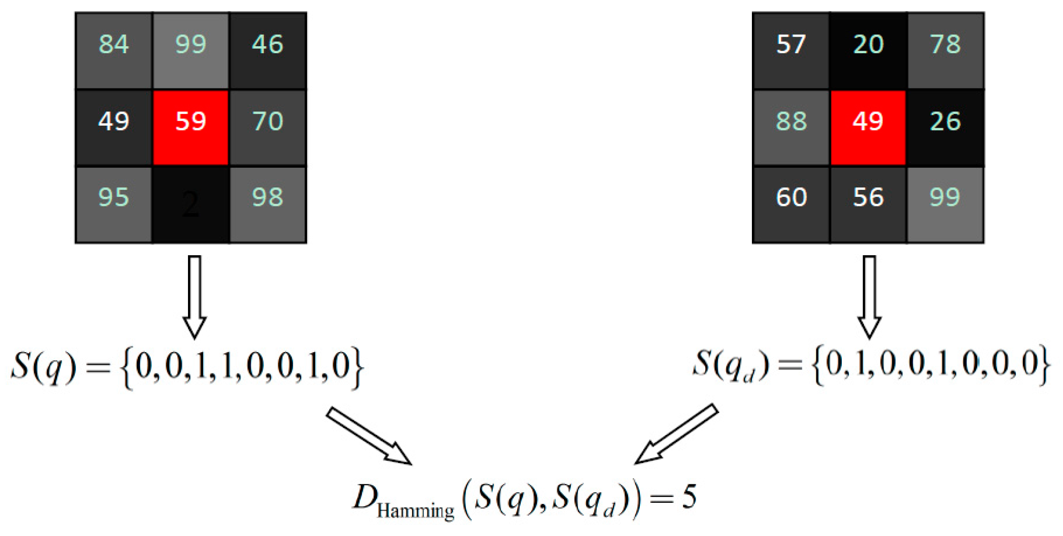
However, greenhouse plant images taken by webcams suffer from problems such as radiometric distortion, low-texture areas (leaves are similar in the same canopy), etc. The raw matching cost computed by TAD is affected by those problems to a large extent. Therefore, we applied an AD-Census measure [42] that combines an absolute difference and a Census transformation to calculate the raw matching cost instead. The principle of Census transformation is given as follows. Firstly, it defines a 3 × 3 window centered at the current pixel, and then compares the grayscale intensity of the current pixel with eight pixels in the window. If a window pixel’s intensity is larger than the center pixel’s intensity, this window pixel is assigned with 0; otherwise, the window pixel is assigned with 1. In this way, the window pixel intensities are transformed into a string containing only 0 and 1. Referring to the example in Figure 8, the string of pixel is denoted by , and the string of pixel is denoted by . The cost of Census transformation is calculated as the Hamming distance between and :
The absolute difference measure is defined as:
Then the AD-Census cost measure is computed as:
in which , are the control parameters for Census cost and AD cost, respectively.
3.4.2. Cost Aggregation
During the step of cost aggregation, the cost is aggregated to measure the dissimilarity between and :
where is a pixel in the reference image, and is the corresponding pixel of with a disparity of on the same row in the target image. and are the aggregation windows centered at and , respectively. Pixel stands for any pixel in , and is a pixel in . The lower the dissimilarity, the higher the chance that matches is.
3.4.3. Disparity Computation and Disparity Refinement
After cost aggregation, the disparity of is selected by using a simple winner-take-all strategy:
Because the disparity acquired from Equation (14) is essentially a difference in pixel position, it results in a discrete disparity and eventually leads to the discrete depth estimation. After triangulation (using Equations (16)–(18)), the point cloud generated by the disparity map obtained from (14) will become layered. In order to solve this problem, a sub-pixel disparity refinement based on quadratic polynomial interpolation [47] is employed to enhance the accuracy. The refinement is shown as in Equation (15):
where denotes the disparity of pixel at coordinate obtained via (14), and is the refined disparity result for pixel . By using Equation (15), each disparity will turn from an integer to a decimal, generating a smoother depth field.
3.5. 3D Point Cloud~Reconstruction
In the last step, we can recover 3D information of each point on disparity surface from the binocular stereo system. As the image pairs are row-aligned and rectified, a series of linear equations can be obtained by triangulation, and then the 3D point cloud of the plant can be calculated:
In the three equations above, is the image coordinate of a pixel, and (X, Y, Z) is the computed inhomogeneous 3D world coordinate of this pixel by triangulation.
4. Results
4.1. Performance of the Proposed Stereo Matching Algorithm
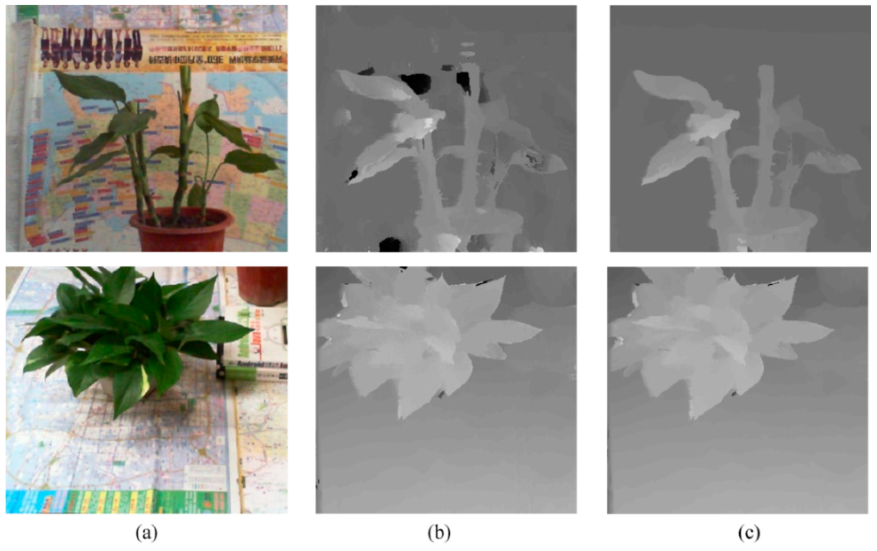
We evaluate the performance of AD-Census cost measure with ASW (the proposed method) against several other stereo matching techniques, including the ASW algorithm [39], Graph Cuts algorithm (GC) [37], and Semi-global Matching (SGBM) algorithm [38] on the Middlebury datasets [48]. The comparative results are shown by disparity maps in Figure 9, which demonstrate that the proposed method can generate disparity images with a higher accuracy than the others. The quantitative analysis is given by Table 1, which shows that our method outperforms the compared methods at most times. The comparative results of the proposed method and the original ASW algorithm on two pairs of real plant images (Epipremnum aureum and Aglaonema modestum) are shown in Figure 10, and it can be observed that the AD-Census cost measure contributes to a better performance because the hollow effect (dark areas) in the disparity map is suppressed.
4.2. Relationship between Accuracy and Baseline
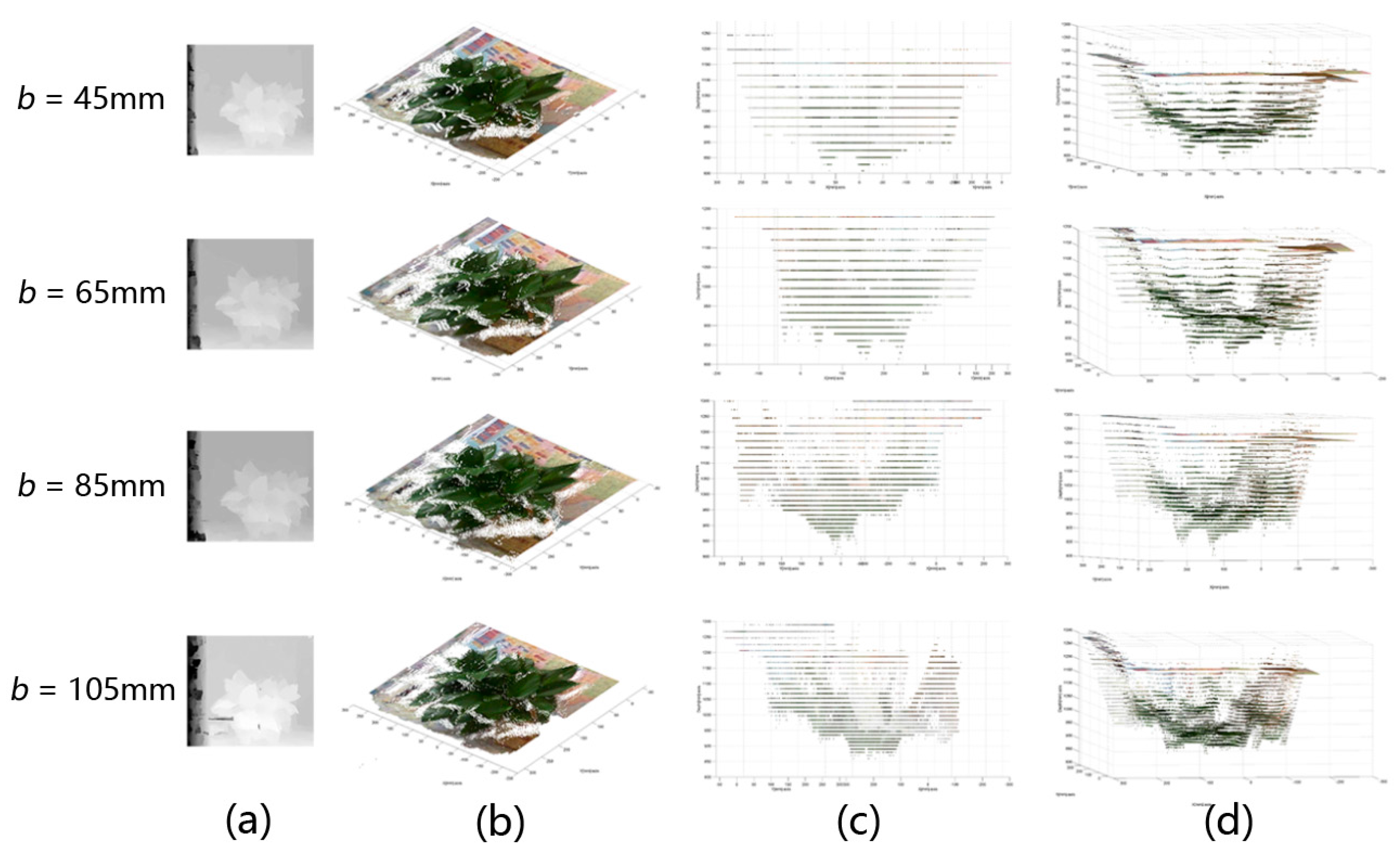
In this subsection, the relationship between the depth accuracy and the length of the baseline is analyzed. This result is also used to provide an optimal baseline for our binocular stereo platform. The plant in Figure 2a is placed within 1 m of the stereo system and we compare the disparity maps generated at four different baseline values: 45 mm, 65 mm, 85 mm, and 105 mm. Figure 11 shows the disparity maps without refinement and corresponding point clouds viewed from three different positions at the four different baseline values, respectively. The results clearly show that the higher the length of the baseline, the more depth layers we will obtain, i.e., the accuracy of depth improves with the increase of baseline length. It can be observed from column (c) in Figure 11 that as the length of baseline increases, the distance between adjacent depth layers in the point cloud decreases. can be computed as follows:
in which and represent the disparities of the two adjacent depth layers, respectively. Because the surface of an object is usually continuous, the disparity between two adjacent layers is 1. Thus can be calculated by:
Based on Equations (19) and (20), it can be concluded that the further away a point is from the stereo system, the larger will be. This is because a distant pixel from a surface must have a small disparity value, which results in a large . This also explains the non-uniform distances between the adjacent layers in column (c) of Figure 11. At the same baseline, the smaller is, the higher accuracy we obtain.
Although the accuracy of depth improves with an increasing baseline length, larger baseline lengths also lead to higher mismatch rates because some of the pixels in the occluded area cannot be observed simultaneously by both cameras. For example, in column (a) of Figure 11, black holes (mismatch) begin to appear in the plant region with a baseline of 105 mm. After comparison, we find that the optimal length of the baseline is around 80 mm because it represents a good trade-off between depth accuracy and mismatch rate for the proposed stereo system. The result is similar for a plant with a distance less than 1 m (e.g., 0.6 m or 0.8 m).
4.3. Reconstruct Point Cloud with Disparity Refinement
The subsection displays the reconstructed 3D point clouds of plants with disparity refinement in three different environments. Figure 12 provides a comparison of 3D point clouds of Epipremnum aureum processed with and without disparity refinement in the indoor lab. It clearly shows that the disparity refinement process by Equation (15) has effectively solved the problem of discrete depth layers.
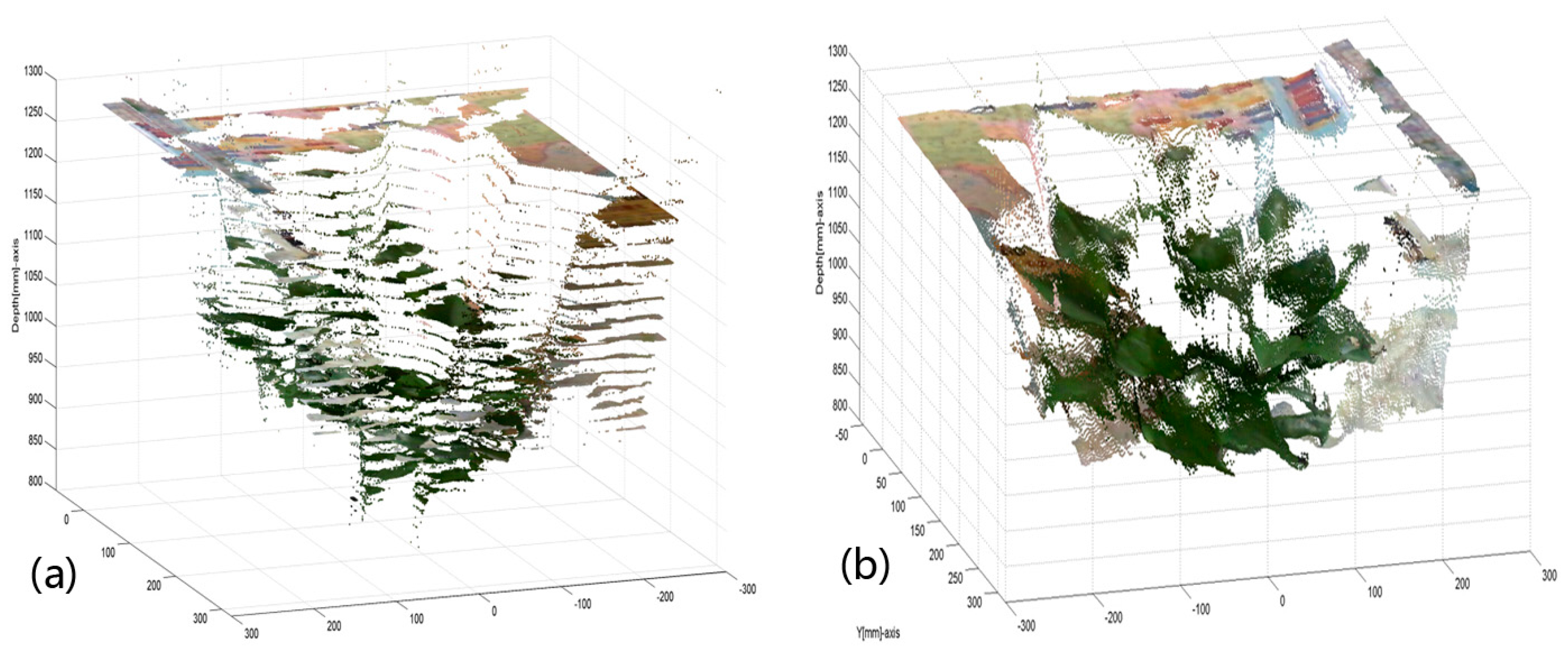
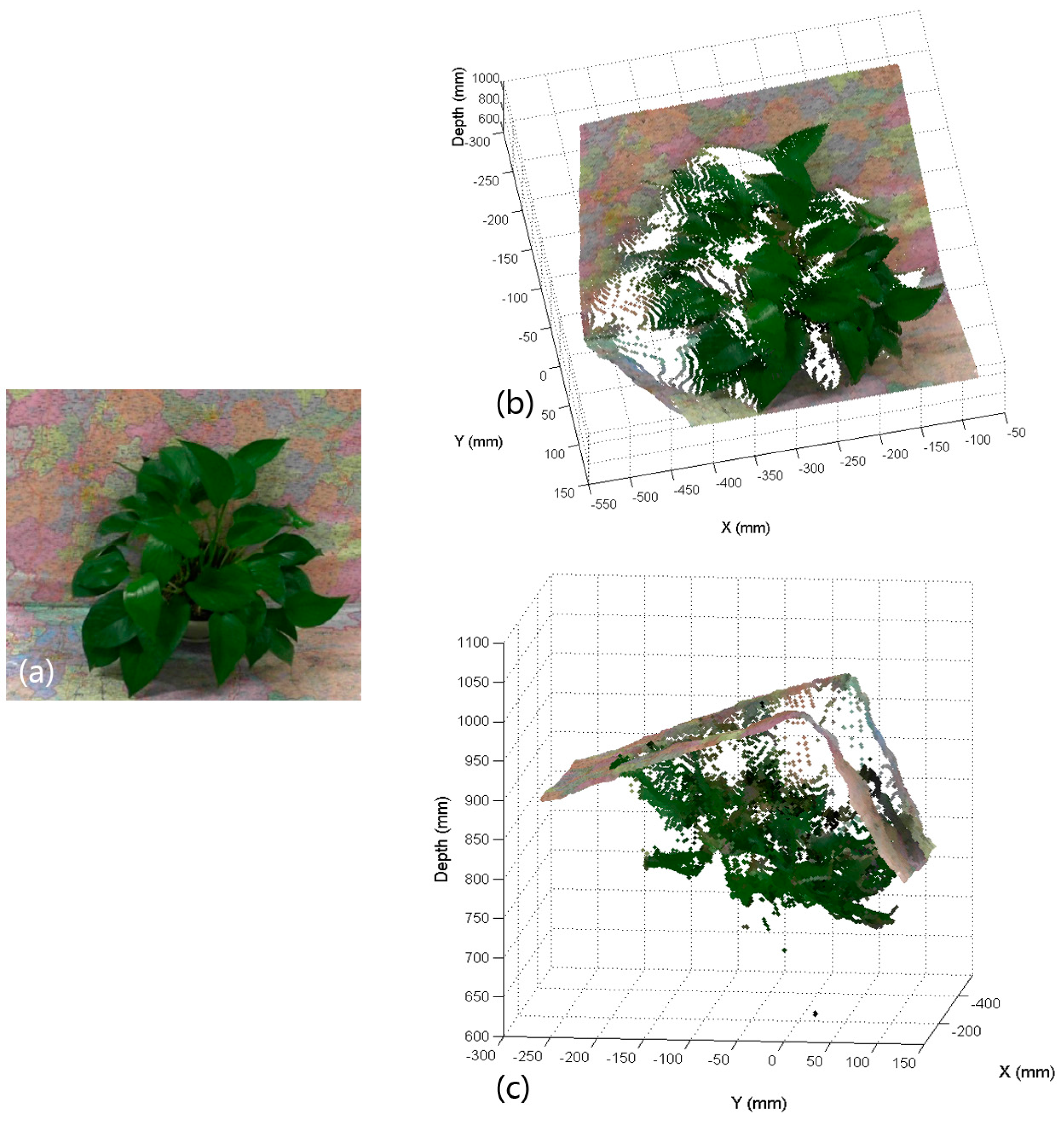
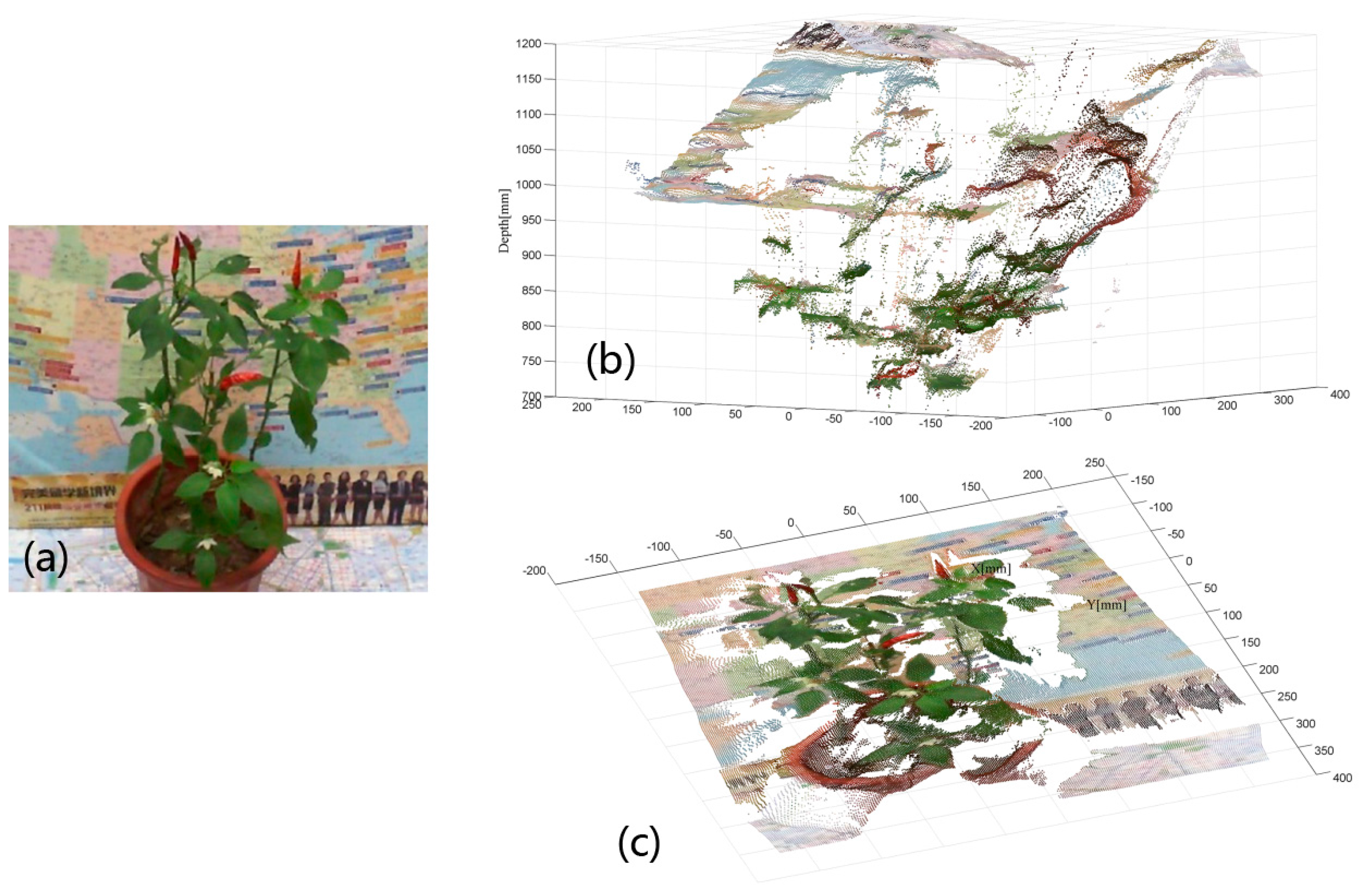
In the lab environment, we used the proposed methodology to carry out 3D point cloud reconstruction with disparity refinement for Epipremnum aureum and the pepper (Capsicum annuum) sample plants. Figure 13 shows the rectified left image and the point cloud of the Epipremnum aureum sample viewed from two different positions. Figure 14 displays the rectified left image and the point cloud of the pepper sample viewed from two different positions.
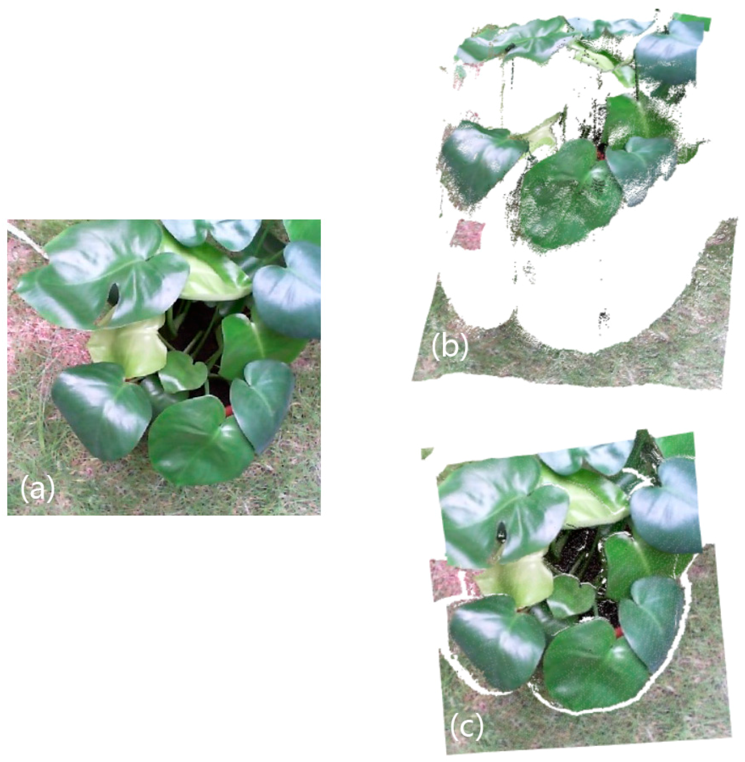
For the environment on an open field, we set up the stereo vision platform and used the proposed methodology to reconstruct a 3D point cloud with disparity refinement for a Monstera deliciosa sample. Figure 15 shows the rectified left image and point cloud of the plant viewed respectively from two different positions.
In the multi-span glass greenhouse located in Jiading campus of Tongji University, we reconstructed 3D point clouds for the potted strawberry sample plants and turnip sample plants, respectively. The stereo-rectified left image and 3D point cloud of the strawberry plants are shown in Figure 16. The stereo-rectified left image and 3D point cloud of the turnip plants are shown in Figure 17.
4.4. Implementation Details
Implementation of the proposed method can be generally divided into five steps. Table 2 lists the information about the software, equipment, URLs for tools, processing time, and data description of each step. The presented ASW stereo matching scheme under AD-Census cost measure costs less than 2 min for a pair of 640 × 480 images, and the final generated point cloud contains more than 170,000 points. The total time of implementation for a new scene is about half an hour. We used our own C++ implementation for the image acquisition, rectification, stereo matching, and 3D reconstruction steps, which are mostly automatic. Only the first two steps of image acquisition and calibration require some manual configurations because of repositioning the chessboard in front of the stereo system and labeling the corner points in Matlab. In application, we only have to calibrate the system only once as the stereo platform is usually fixed on site. Then the growth of the greenhouse plant can be monitored by conducting a continuous 3D reconstruction that only takes several minutes at each image pair.
5. Discussion
5.1. Depth Error
Error of depth originates from three major aspects: calibration error, foreshortening error and misalignment error. The calibration error results from inaccurate estimation of the extrinsic as well as the intrinsic camera parameters. Calibration inaccuracy further leads to 2D reprojection error in the image plane, and finally causes a 3D localization error. The foreshortening error is caused by a 3D scene that is not fronto-parallel. The misalignment error is caused by mismatch in the stereo matching process. In order to analyze the depth estimation error, a theoretical error model [49] between the disparity error and the depth error is established as follows:
According to this definition, the disparity is the difference of horizontal coordinates between the left image and the right image on the same epipolar line, therefore we have . Then the error of disparity can be represented as:
Due to the discrete nature of digital imaging systems, the image coordinates are inevitably influenced by quantization noise. This means and can be up to half of a pixel in magnitude. Assuming is uniformly distributed, and the imaging processes of two cameras in the binocular system are mutually independent, then we obtain:
where is the image sampling interval that determines the image resolutions. In our work, the sensor size of the webcam is about 1/2” (width 6.4 mm, height 4.8 mm), and the images are taken at the resolution of 1280 × 720. As the disparity is calculated in the horizontal direction, the image sampling interval is calculated as mm, which means that in the worst case the error of disparity can reach up to 0.005 mm. According to the calibration step, the focal length of the webcam is 3.9 mm. If the baseline is fixed at 85 mm, and the object being measured is placed 1.0 m away from the stereo system, the absolute value of depth error has an upper bound of 14.86 mm when applying Equation (21). If the object-to-camera distance is less than 0.8 m, the error will be no higher than 10 mm according to Equation (21).
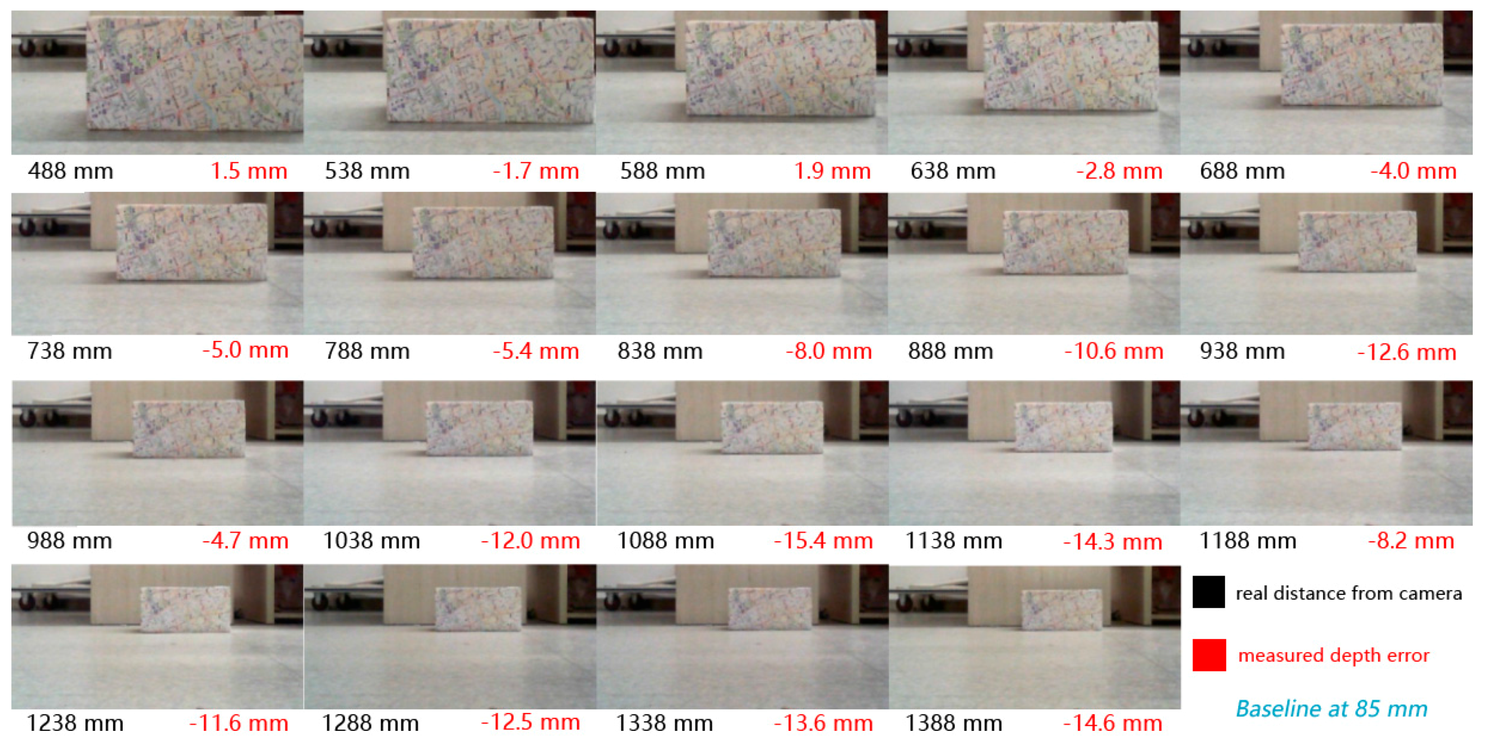
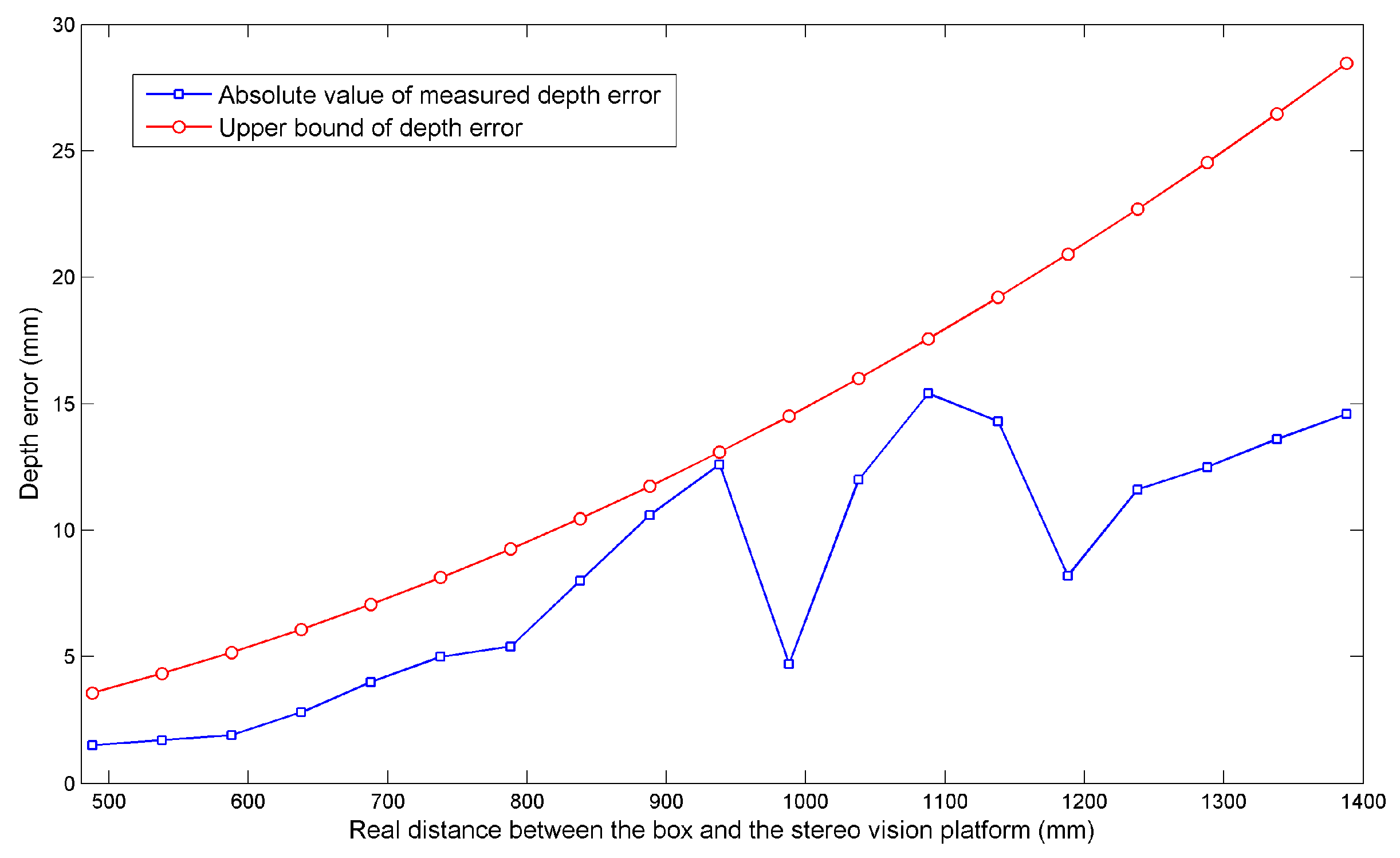
In order to quantitatively measure the actual depth errors, we place a textured box in front of the cameras and compare its real distance to the stereo platform with the distance computed by Equation (18). The real distance between the box and cameras varies in the range of 488 mm to 1388 mm with a step of 50 mm. Nineteen image pairs are recorded in the range, and the left images are shown in Figure 18. The measured depth error is defined as the difference between the real distance and the distance computed by triangulation, and Figure 19 plots the absolute measured depth errors and the upper bounds computed from the theoretical model at 19 different ranges. In this figure, we can see that the two depth error curves both increase with the distance between the object surface and the stereo platform, and the quantitative results comply with the theoretical model given by Equation (21). For an object that is less than 800 mm away from the stereo system, the measured depth error is less than 5 mm. According to our manual measurement, the average leaf length and width of Epipremnum aureum sample plant are approximately 103.6 mm and 56.4 mm, respectively. The average leaf length and width of Aglaonema modestum sample plant are approximately 146.7 mm and 62.2 mm, respectively. The average leaf length and width of the sample pepper plant used in experiment are approximately 70.8 mm and 35.0 mm, respectively. Compared to the average leaf sizes of the three test plants, the measured depth error of our system is tolerable.
When the disparity is close to 0, small differences in disparity lead to large depth fluctuations. Contrarily, when disparity is large, small disparity variations do not significantly change the depth. This means that this binocular stereo platform has high depth accuracy only for objects that are close to the cameras. As the distance between the object and the cameras increases, the pixel resolution of the object decreases, leading to a larger error of depth measurements.
5.2. Feasibility
The proposed methodology is feasible for greenhouses and even outdoor environments. We are particularly concerned with the performance and stability of the inexpensive stereo vision platform in greenhouses. Thus different kinds of devices were tested for the platform in our automated greenhouse. Three different webcam pairs with inexpensive prices, including HD-3000 Series (Microsoft, Redmond, WA, USA), LifeCam Studio (Microsoft, Redmond, WA, USA), and TTQ Series (Kingyo Century Technology Development Co. Ltd., Shenzhen, China) were tested and compared. They showed reliable results, and their respective plant point clouds are also quite similar. It is also noteworthy that these webcams all endured high humidity and temperature in our greenhouse for several days, which indicates the feasibility of using ordinary webcams in this situation.
In our system, a laptop is connected to the vision platform to capture and process stereo data. Although a laptop works favorably in the lab environment, it is not clear whether it can work normally for a period of time in a greenhouse with high humidity and extra heat. Therefore we tested two different laptops in the greenhouse—one is an Acer (4830T series, Acer, New Taipei City, Taiwan); the other is a Dell (XPS15-9550, Dell, Round Rock, TX, USA). Each laptop endured a two-day experiment in the greenhouse, and both worked normally during the period of testing. This result supports the applicability of our methodology to greenhouse imaging.
5.3. Invariance against Illumination Changes
The proposed 3D imaging system shows invariance against changing illumination in various greenhouse experiments. We fixed the poses and orientations of our stereo platform during imaging, and captured image pairs under different illumination conditions to carry out point cloud generation. For the strawberry plants, we compared image pairs obtained in overcast and sunny weather. In Figure 20, both cases show satisfactory disparities, and the point clouds are almost identical. For greenhouse turnips, the image pairs were also captured under different illuminations. Figure 21 shows the disparity comparison and turnip point clouds in two views, which also exhibit the invariances against illumination changes. Therefore, our method is robust against illumination changes in a real greenhouse.
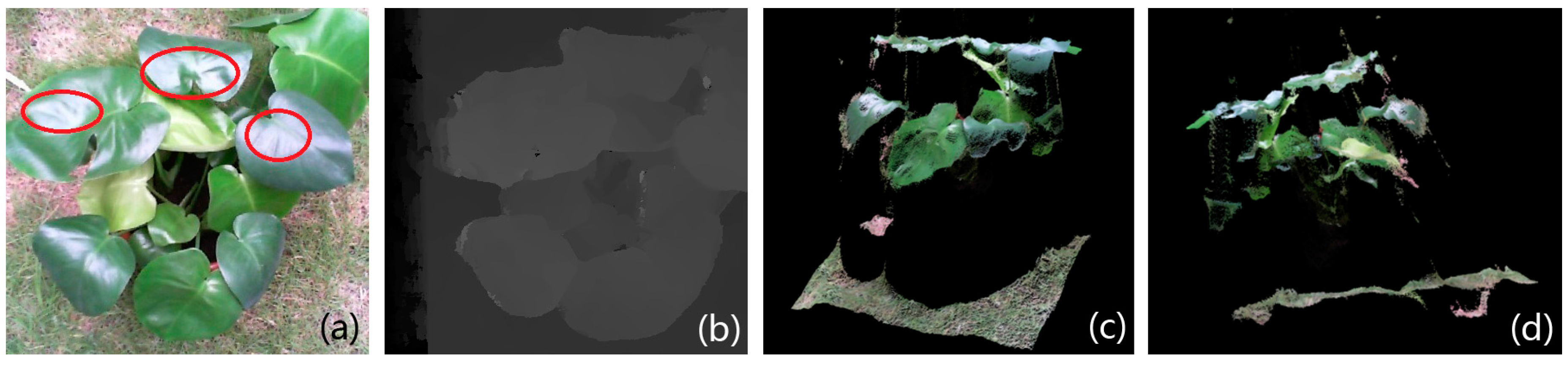
Highlighting is another challenge created by illumination in plant imaging. It is often observed on the surfaces of large and smooth leaves because of the specular reflection of sunlight. A highlight region usually takes on bright white color; hence the highlighted region loses texture details, creating obstacles for many stereo matching algorithms. Monstera deliciosa has broad and smooth leaves so it is an ideal sample for testing the performance of the presented method when highlights appear. In the outdoor experiment, several highlight regions labeled by red ellipses can be observed in Figure 22a. Our stereo matching algorithm successfully generated a satisfactory disparity map, shown in Figure 22b, in which the highlighted regions had stable disparity. The two views of the final reconstructed point cloud of the sample (Figure 22c,d) show that we not only recovered individual leaves, but also recovered the local curvature of each leaf. It can be seen that the regions without highlight are mostly rugged, which coincides with the fact that highlight only comes from smooth and flat surfaces. The invariance against highlight can be explained by looking into the theory of the proposed stereo matching scheme. In a highlighted region, the pixels take on uniform and saturated color. Though most of such a region is low-textured, the boundary of the region still has a sharp intensity gradient. The AD-Census measure can record the intensity gradients around the two compared pixels. After the cost aggregation step (Equation (13)), the gradient information is enhanced. Once the aggregation window is large enough to incorporate edges from a highlighted region, the disparity can be correctly computed based on the aggregated gradient information.
5.4. Leaves Segmentation
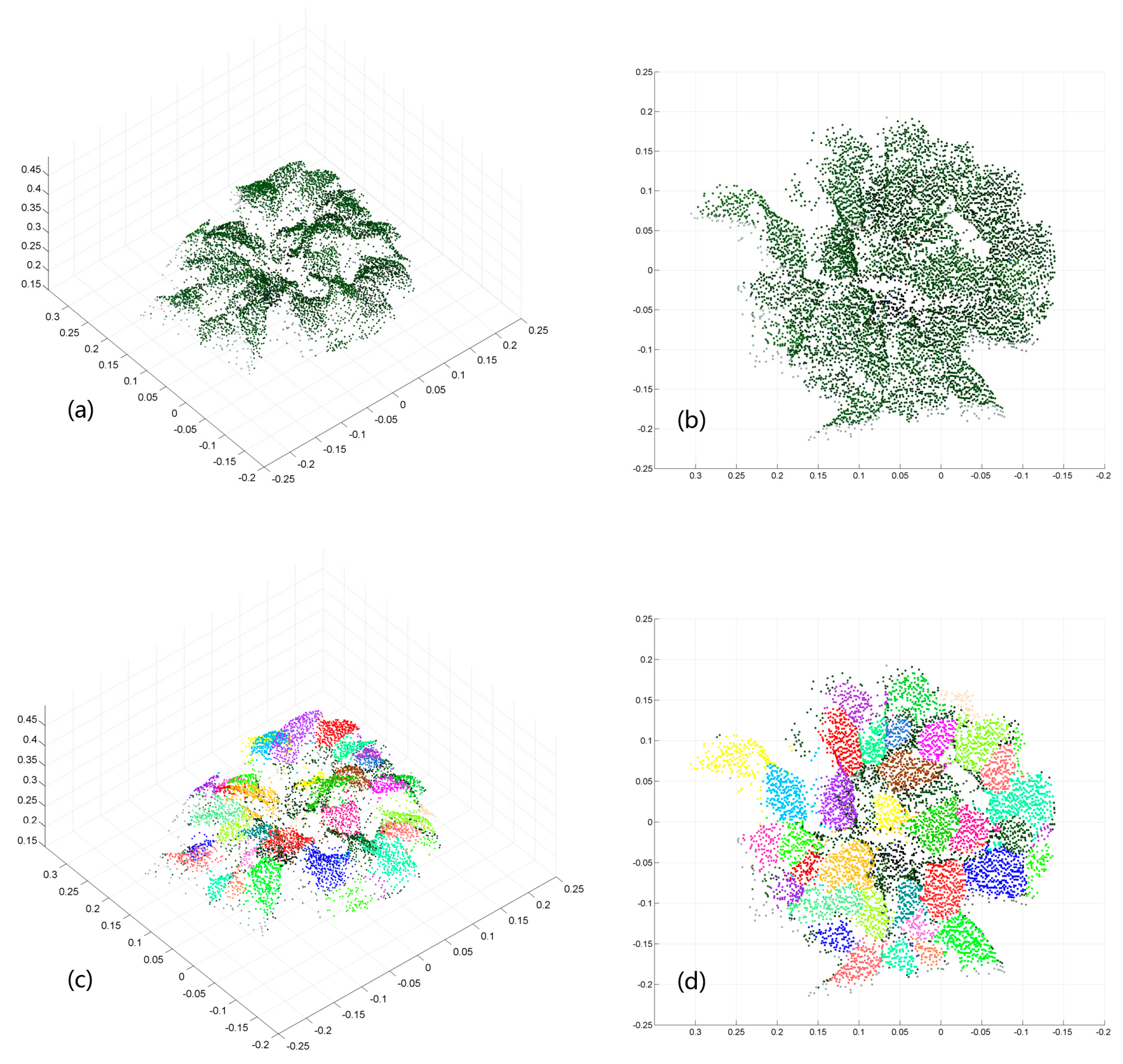
A successful segmentation relies on a dense and accurate point cloud because it contains richer features than low-quality point clouds. Hence it is reasonable to validate the quality of the point cloud by assessing the segmentation results. In this subsection, we try to segment leaves individually from the point cloud of Epipremnum aureum generated by our methodology to validate the quality of the point cloud. Figure 23a,b display the side and top view, respectively, of the Epipremnum aureum point cloud containing only canopy. This point cloud was obtained from the point cloud shown in Figure 13 by using a green color filter. The Octree data structure was used to process points in the cloud, and for each seed point we traverse its K nearest neighborhood points. The neighborhood points that satisfy both similar 3D positions and similar normal with the seed point are regarded as part of a same leaf, and are segmented with a uniform color. Figure 23c,d are the segmentation results corresponding to (a) and (b), respectively. The segmentation scheme shows a satisfactory performance, recognizing 35 of the 37 true leaves. This reveals that our method successfully recovers the 3D curvature of each leaf of the Epipremnum aureum sample plant.
6. Conclusions
For the purpose of serving greenhouse cultivation and advancing high-throughput plant phenotyping, a low-cost and portable stereo vision system is established to realize 3D imaging of greenhouse plants. Our platform does not place harsh limitations on cameras and laptops in greenhouse experiments, which indicates high feasibility. In the stereo matching step, an efficient cost calculating measure—AD-Census—is integrated with the ASW algorithm to improve the latter’s performance on real plant images. In the quantitative assessment, our stereo algorithm reaches an average error rate of 6.63% on the Middlebury datasets, lower than rates of the original ASW approach and several other popular algorithms. The imaging accuracy of the proposed method under different baseline settings is investigated. The experimental results show that the optimal length of baseline is approximately 80 mm for reaching a good trade-off between the depth accuracy and the mismatch rate for a plant within 1 m distance. The theoretical error analysis (red curve in Figure 19) shows that for an object within 1 m distance, the depth error has an upper bound of 14.86 mm; and for an object with less than 800 mm distance, the depth error is no higher than 10 mm. The experimental error analysis (blue curve in Figure 19) shows that for an object less than 800 mm away from our stereo system, the absolute value of actually measured depth error is no higher than 5 mm. Although the measured error curve fluctuates in the distance range 800–1200 mm, the measured value is lower than the theoretical upper bound (especially when the distance is near 1 m, the absolute measured depth error falls to 4.7 mm). This error is tolerable considering the dimensions of greenhouse plants. By applying disparity refinement, the proposed methodology generates dense and accurate point clouds of crops in different environments including an indoor lab, an outdoor field, and a greenhouse. It also shows invariance against changing illumination in greenhouses, as well as the ability to recover the 3D surfaces of the highlighted leaf regions.
As our binocular platform only recovers the 3D point cloud from two views, sometimes partial occlusion is unavoidable. In the future, we will focus on applying the proposed stereo matching algorithm on multi-view stereo systems, and designing a highly reliable point cloud registration method to acquire complete point clouds of greenhouse plants. Our ultimate goal is to recognize the growth status of the crops in real time via 3D imaging and phenotyping of their organs.
Supplementary Materials
The following are available online at www.mdpi.com/2072-4292/9/5/508/s1, Video S1: Monstera deliciosa L. point cloud.mp4. Video S1 is the video of the point cloud of a Monstera deliciosa sample plant. Some screenshots of this video are also displayed in Figure 15 and Figure 22. Video S2: Strawberry point cloud.mp4. Video S2 is the video of the point clouds of several strawberry plants cultivated in the greenhouse. Some screenshots of this video are also displayed in Figure 16 and Figure 20. Video S3: Turnip crop point cloud.mp4. Video S3 is the video of the point clouds of several turnip plants cultivated in the greenhouse. Some screenshots of this video are also displayed in Figure 17 and Figure 21. Video S4: Leaves segmentation displayed in Matlab (medium quality) .mp4. Video S4 shows the point cloud of the Epipremnum aureum sample plant after automatic leaves segmentation. Some screenshots of this video are also displayed in Figure 23.
Acknowledgments
This work was jointly supported by the National High-Tech R&D Program of China under Grant 2013AA102305; the Natural Science Foundation of China under Grants 61603089, 61603090, and 61573258; Shanghai Sailing Programs 16YF1400100, 17YF1426100; the Fundamental Research of the Shanghai Committee of Science and Technology under Grant 15JC1400600; the fundamental Research Funds for the Central Universities of China under Grant 233201600068; and the U.S. National Science Foundation’s BEACON Center for the Study of Evolution in Action, under cooperative agreement DBI-0939454.
Author Contributions
The theoretical derivations were done by Dawei Li and Lihong Xu; Peng Zhang and Shaoyuan Sun designed the experiments; Dawei Li and Xue-song Tang organized the experimental data and wrote the paper; Xin Cai carried out part of the experiments.
Conflicts of Interest
The authors declare no conflict of interest.
References
- Fahlgren, N.; Gehan, M.A.; Baxter, I. Lights, camera, action: High-throughput plant phenotyping is ready for a close-up. Curr. Opin. Plant Biol. 2015, 24, 93–99. [Google Scholar] [CrossRef] [PubMed]
- Romeo, J.; Pajares, G.; Montalvo, M.; Guerrero, J.M.; Guijarro, M.; Cruz, J.M.D.L. A new Expert System for Greeness Identification in Agricultural Images. Expert Syst. Appl. 2013, 40, 2275C2286. [Google Scholar] [CrossRef]
- Montalvo, M.; Guerrero, J.M.; Romeo, J.; Emmi, L.; Guijarro, M.; Pajares, G. Automatic expert system for weeds/crops identification in images from maize fields. Expert Syst. Appl. 2013, 40, 75–82. [Google Scholar] [CrossRef]
- Meyer, G.E.; Neto, J.C.; Jones, D.D.; Hindman, T.W. Intensified fuzzy clusters for classifying plant, soil, and residue regions of interest from color images. Comput. Electron. Agric. 2004, 42, 161–180. [Google Scholar] [CrossRef]
- Bruno, O.M.; Plotze, R.D.O.; Falvo, M.; Castro, M.D. Fractal dimension applied to plant identification. Inform. Sci. 2008, 178, 2722–2733. [Google Scholar] [CrossRef]
- Backes, A.R.; Casanova, D.; Bruno, O.M. Plant Leaf Identification Based On Volumetric Fractal Dimension. Int. J. Pattern Recognit. Artif. Intell. 2011, 23, 1145–1160. [Google Scholar] [CrossRef]
- Neto, J.C.; Meyer, G.E.; Jones, D.D. Individual leaf extractions from young canopy images using GustafsonCKessel clustering and a genetic algorithm. Comput. Electron. Agric. 2006, 51, 66–85. [Google Scholar] [CrossRef]
- Zeng, Q.; Miao, Y.; Liu, C.; Wang, S. Algorithm based on marker-controlled watershed transform for overlapping plant fruit segmentation. Opt. Eng. 2009, 48, 027201. [Google Scholar] [CrossRef]
- Xu, G.; Zhang, F.; Shah, S.G.; Ye, Y.; Mao, H. Use of leaf color images to identify nitrogen and potassium deficient tomatoes. Pattern Recognit. Lett. 2011, 32, 1584–1590. [Google Scholar] [CrossRef]
- Scharr, H.; Minervini, M.; French, A.P.; Klukas, C.; Kramer, D.M.; Liu, X.; Luengo, I.; Pape, J.-M.; Polder, G.; Vukadinovic, D.; et al. Leaf segmentation in plant phenotyping: A collation study. Mach. Vis. Appl. 2015, 27, 585–606. [Google Scholar] [CrossRef]
- Pape, J.M.; Klukas, C. 3-D histogram-based segmentation and leaf detection for rosette plants. In ECCV 2014 Workshops; Springer: Cham, Switzerland, 2015; Volume 8928, pp. 61–74. [Google Scholar]
- Achanta, R.; Shaji, A.; Smith, K.; Lucchi, A.; Fua, P.; Susstrunk, S. SLIC superpixels compared to state-of-the-art superpixel methods. IEEE Trans. Pattern Anal. Mach. Intell. 2012, 34, 2274–2282. [Google Scholar] [CrossRef] [PubMed]
- Yin, X.; Liu, X.; Chen, J.; Kramer, D.M. Multi-leaf alignment from fluorescence plant images. In Proceedings of the IEEE Winter Conference on Applications of Computer Vision (WACV), Steamboat Springs, CO, USA, 24–26 March 2014; pp. 437–444. [Google Scholar]
- Barrow, H.G.; Tenenbaum, J.M.; Bolles, R.C.; Wolf, H.C. Parametric Correspondence and Chamfer Matching: Two New Techniques for Image Matching. In Proceedings of the 5th International Joint Conference on Artificial Intelligence (IJCAI’77), Cambridge, MA, USA, 22–25 August 1977; Volume 2, pp. 659–663. [Google Scholar]
- Fernandez, R.; Montes, H.; Salinas, C.; Sarria, J.; Armada, M. Combination of RGB and Multispectral Imagery for Discrimination of Cabernet Sauvignon Grapevine Elements. Sensors 2013, 13, 7838–7859. [Google Scholar] [CrossRef] [PubMed]
- Li, H.; Lee, W.S.; Wang, K. Identifying blueberry fruit of different growth stages using natural outdoor color images. Comput. Electron. Agric. 2014, 106, 91–101. [Google Scholar] [CrossRef]
- Sansoni, G.; Trebeschi, M.; Docchio, F. State-of-The-Art and Applications of 3D Imaging Sensors in Industry, Cultural Heritage, Medicine, and Criminal Investigation. Sensors 2009, 9, 568–601. [Google Scholar] [CrossRef] [PubMed]
- Nguyen, D.V.; Kuhnert, L.; Kuhnert, K.D. Structure overview of vegetation detection. A novel approach for efficient vegetation detection using an active lighting system. Robot. Auton. Syst. 2012, 60, 498–508. [Google Scholar] [CrossRef]
- Alenya, G.; Dellen, B.; Torras, C. 3D modelling of leaves from color and ToF data for robotized plant measuring. In Proceedings of the IEEE International Conference on Robotics and Automation (ICRA), Shanghai, China, 9–13 May 2011; pp. 3408–3414. [Google Scholar]
- Fernández, R.; Salinas, C.; Montes, H.; Sarria, J. Multisensory System for Fruit Harvesting Robots. Experimental Testing in Natural Scenarios and with Different Kinds of Crops. Sensors 2014, 14, 23885–23904. [Google Scholar] [CrossRef] [PubMed]
- Garrido, M.; Paraforos, D.; Reiser, D.; Vzquez Arellano, M.; Griepentrog, H.; Valero, C. 3D Maize Plant Reconstruction Based on Georeferenced Overlapping LiDAR Point Clouds. Remote Sens. 2015, 7, 17077–17096. [Google Scholar] [CrossRef]
- Seidel, D.; Beyer, F.; Hertel, D.; Fleck, S.; Leuschner, C. 3D-laser scanning: A non-destructive method for studying above- ground biomass and growth of juvenile trees. Agric. Forest Meteorol. 2011, 151, 1305–1311. [Google Scholar] [CrossRef]
- Xu, H.; Gossett, N.; Chen, B. Knowledge and heuristic-based modeling of laser-scanned trees. ACM Trans. Graph. 2007, 26, 377–388. [Google Scholar] [CrossRef]
- Dassot, M.; Colin, A.; Santenoise, P.; Fournier, M.; Constant, T. Terrestrial laser scanning for measuring the solid wood volume, including branches, of adult standing trees in the forest environment. Comput. Electron. Agric. 2012, 89, 86–93. [Google Scholar] [CrossRef]
- Dornbusch, T.; Wernecke, P.; Diepenbrock, W. A method to extract morphological traits of plant organs from 3D point clouds as a database for an architectural plant model. Ecol. Modelling 2007, 200, 119–129. [Google Scholar] [CrossRef]
- Li, Y.; Fan, X.; Mitra, N.J.; Chamovitz, D.; Cohen-Or, D.; Chen, B. Analyzing growing plants from 4D point cloud data. ACM Trans. Graph. 2013, 32, 1–10. [Google Scholar] [CrossRef]
- Paulus, S.; Behmann, J.; Mahlein, A.K.; Kuhlmann, H. Low-cost 3D systems: Suitable tools for plant phenotyping. Sensors 2014, 14, 3001–3018. [Google Scholar] [CrossRef] [PubMed]
- Chn, Y.; Rousseau, D.; Lucidarme, P.; Bertheloot, J.; Caffier, V.; Morel, P.; Tienne, B.; Chapeau-Blondeau, F. On the use of depth camera for 3D phenotyping of entire plants. Comput. Electron. Agric. 2012, 82, 122–127. [Google Scholar] [CrossRef]
- Li, D.; Xu, L.; Tan, C.; Goodman, E.D.; Fu, D.; Xin, L. Digitization and visualization of greenhouse tomato plants in indoor environments. Sensors 2015, 15, 4019–4051. [Google Scholar] [CrossRef] [PubMed]
- Yamamoto, S.; Hayashi, S.; Tsubota, S. Growth measurement of a community of strawberries using three-dimensional sensor. Environ. Control. Biol. 2015, 53, 49–53. [Google Scholar] [CrossRef]
- Schima, R.; Mollenhauer, H.; Grenzdorffer, G.; Merbach, I.; Lausch, A.; Dietrich, P.; Bumberger, J. Imagine all the plants: Evaluation of a light-field camera for on-site crop growth monitoring. Remote Sens. 2016, 8, 823. [Google Scholar] [CrossRef]
- Apelt, F.; Breuer, D.; Nikoloski, Z.; Stitt, M.; Kragler, F. Phytotyping 4D: A light-field imaging system for non-invasive and accurate monitoring of spatio-temporal plant growth. Plant J. 2015, 82, 693–706. [Google Scholar] [CrossRef] [PubMed]
- Biskup, B.; Scharr, H.; Schurr, U.; Rascher, U. A stereo imaging system for measuring structural parameters of plant canopies. Plant Cell Environ. 2007, 30, 1299C1308. [Google Scholar] [CrossRef] [PubMed]
- Teng, C.H.; Kuo, Y.T.; Chen, Y.S. Leaf segmentation, classification, and three-dimensional recovery from a few images with close viewpoints. Opt. Eng. 2011, 50, 103–108. [Google Scholar]
- Hu, P.; Guo, Y.; Li, B.; Zhu, J.; Ma, Y. Three-dimensional reconstruction and its precision evaluation of plant architecture based on multiple view stereo method. Trans. Chin. Soc. Agric. Eng. 2015, 31, 209–214. [Google Scholar]
- Duan, T.; Chapman, S.C.; Holland, E.; Rebetzke, G.J.; Guo, Y.; Zheng, B. Dynamic quantification of canopy structure to characterize early plant vigour in wheat genotypes. J. Exp. Botany 2016, 67, 4523–4534. [Google Scholar] [CrossRef] [PubMed]
- Boykov, Y.; Veksler, O.; Zabih, R. Fast approximate energy minimization via graph cuts. IEEE Trans. Pattern Anal. Mach. Intell. 2001, 23, 1222–1239. [Google Scholar] [CrossRef]
- Hirschmuller, H. Stereo processing by semiglobal matching and mutual information. IEEE Trans. Pattern Anal. Mach. Intell. 2008, 30, 328–341. [Google Scholar] [CrossRef] [PubMed]
- Yoon, K.J.; Kweon, I.S. Adaptive support-weight approach for correspondence search. IEEE Trans. Pattern Anal. Mach. Intell. 2006, 28, 650–656. [Google Scholar] [CrossRef] [PubMed]
- Hosni, A.; Rhemann, C.; Bleyer, M.; Rother, C.; Gelautz, M. Fast cost-volume filtering for visual correspondence and beyond. IEEE Trans. Pattern Anal. Mach. Intell. 2013, 35, 504–511. [Google Scholar] [CrossRef] [PubMed]
- Hosni, A.; Bleyer, M.; Gelautz, M. Secrets of adaptive support weight techniques for local stereo matching. Comput. Vis. Image Underst. 2013, 117, 620–632. [Google Scholar] [CrossRef]
- Mei, X.; Sun, X.; Zhou, M.; Jiao, S.; Wang, H.; Zhang, X. On building an accurate stereo matching system on graphics hardware. In Proceedings of the IEEE International Conference on Computer Vision Workshops, ICCV 2011 Workshops, Barcelona, Spain, 6–13 November 2011; pp. 467–474. [Google Scholar]
- Bouguet, J.Y. Camera Calibration Toolbox for MATLAB. Available online: http://www.vision.caltech.edu/bouguetj/calib_doc/ (accessed on 14 October 2015).
- Zhang, Z. A Flexible New Technique for Camera Calibration. IEEE Trans. Pattern Anal. Mach. Intell. 2000, 22, 1330–1334. [Google Scholar] [CrossRef]
- Tombari, F.; Mattoccia, S.; Stefano, L.D.; Addimanda, E. Classification and evaluation of cost aggregation methods for stereo correspondence. In Proceedings of the IEEE Conference on Computer Vision and Pattern Recognition, Anchorage, AK, USA, 23–28 June 2008; pp. 1–8. [Google Scholar]
- Scharstein, D.; Szeliski, R. A Taxonomy and Evaluation of Dense Two-Frame Stereo Correspondence Algorithms. Int. J. Comput. Vis. 2002, 47, 131–140. [Google Scholar] [CrossRef]
- Yang, Q.; Wang, L.; Yang, R.; Stewnius, H.; Nistr, D. Stereo matching with color-weighted correlation, hierarchical belief propagation, and occlusion handling. IEEE Trans. Pattern Anal. Mach. Intell. 2008, 31, 492–504. [Google Scholar] [CrossRef] [PubMed]
- Middlebury Stereo Evaluation-Version 2. Available online: http://vision.middlebury.edu/stereo/eval (accessed on 22 March 2015).
- Chang, C.; Chatterjee, S. Quantization error analysis in stereo vision. In Proceedings of the 1992 Conference Record of The Twenty-Sixth Asilomar Conference on Signals, Systems and Computers, Pacific Grove, CA, USA, 26–28 October 1992; Volume 2, pp. 1037–1041. [Google Scholar]
Figure 1.
The established low-cost, portable binocular stereo vision system.

Figure 2.
Six types of greenhouse plants were used in experiments. (a) Epipremnum aureum; (b) Aglaonema modestum; (c) pepper plant; (d) Monstera deliciosa; (e) greenhouse strawberry plants; and (f) greenhouse turnip plants.
Figure 2.
Six types of greenhouse plants were used in experiments. (a) Epipremnum aureum; (b) Aglaonema modestum; (c) pepper plant; (d) Monstera deliciosa; (e) greenhouse strawberry plants; and (f) greenhouse turnip plants.

Figure 3.
The 3D imaging experiments for sample plants were carried out in three environments: (a) an indoor lab of Donghua University, (b) an open field in Donghua University, and (c) a multi-span glass greenhouse in Tongji University.
Figure 3.
The 3D imaging experiments for sample plants were carried out in three environments: (a) an indoor lab of Donghua University, (b) an open field in Donghua University, and (c) a multi-span glass greenhouse in Tongji University.
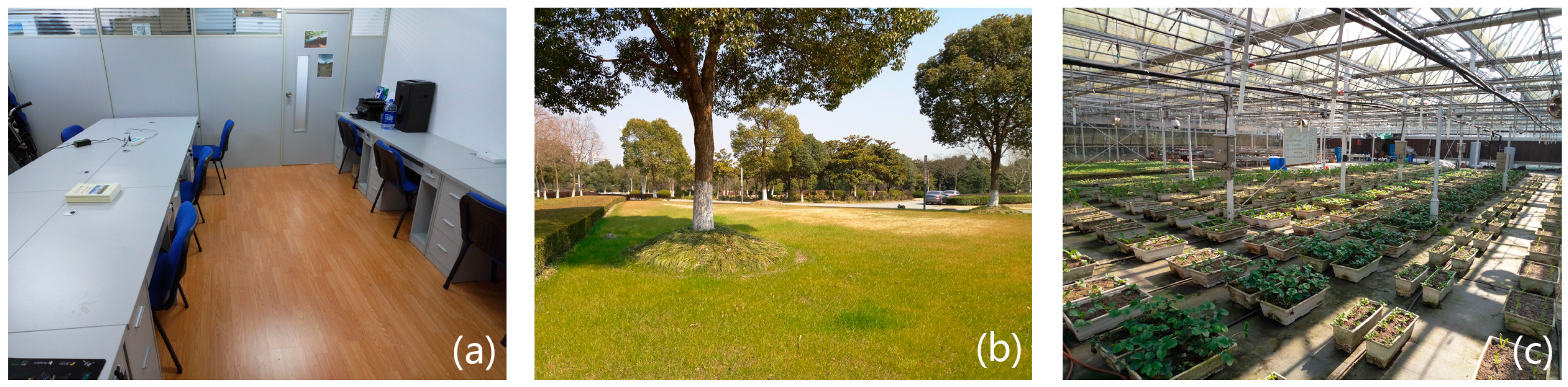
Figure 4.
A plot of epipolar geometry of a binocular stereo vision system.
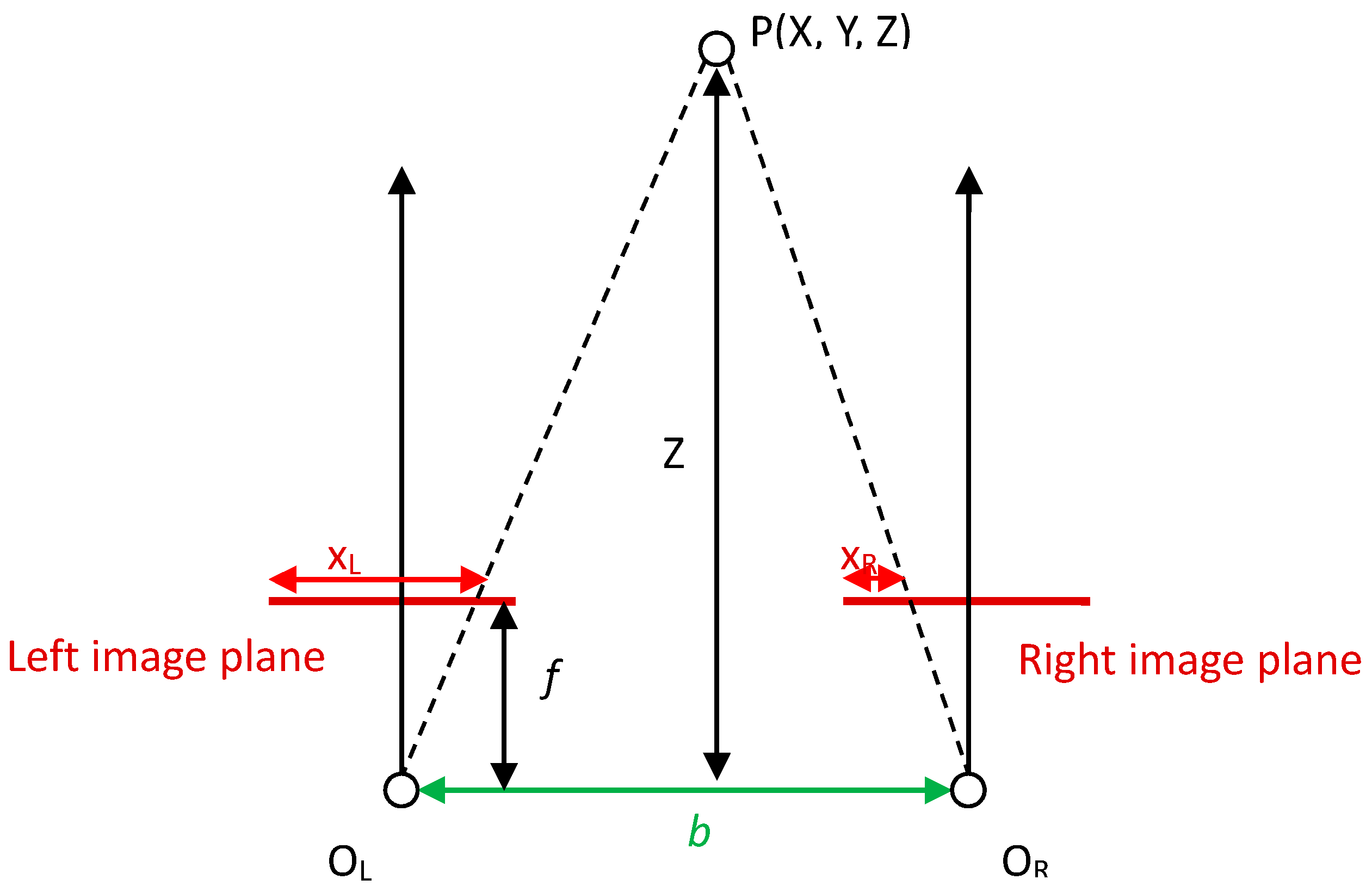
Figure 5.
Working principle of the proposed binocular stereo vision system. The procedure of imaging consists of four steps—(i) camera calibration, (ii) stereo rectification, (iii) stereo matching and (iv) 3D point cloud reconstruction. The left column of this figure (a,c,e,g) shows the methodology and equipment used in the four steps, and the right column (b,d,f,h) shows intermediate and final results step by step. Figure 5a shows the stereo vision platform that contains two webcams and an image pair of a chessboard used for calibration. (b) Records of the spatial positions of the camera system and the chessboard during calibration, realized by using the Camera Calibration Toolbox for Matlab [43]. Stereo rectification aligns the epipolar lines of the left and the right cameras and reduces the camera distortion near the image boundaries, and after rectification, the correspondence search in stereo matching can be reduced from 2D to 1D. (c) The stereo rectification corresponds to paralleling the principal axis of a camera to the other. (d) After the rectification, the camera distortion around image boundaries is reduced. (e) Disparity is formed by two different image planes; (f) the disparity map generated by using stereo matching algorithms. (g) The mapping between the disparity map to the real 3D space by triangulation; (h) the final 3D point cloud.

Figure 6.
Calibration using a two-side chessboard. (a,b) are two images of one side with 8 × 8 grids. (c,d) are two images of the other side with 10 × 10 grids.
Figure 6.
Calibration using a two-side chessboard. (a,b) are two images of one side with 8 × 8 grids. (c,d) are two images of the other side with 10 × 10 grids.
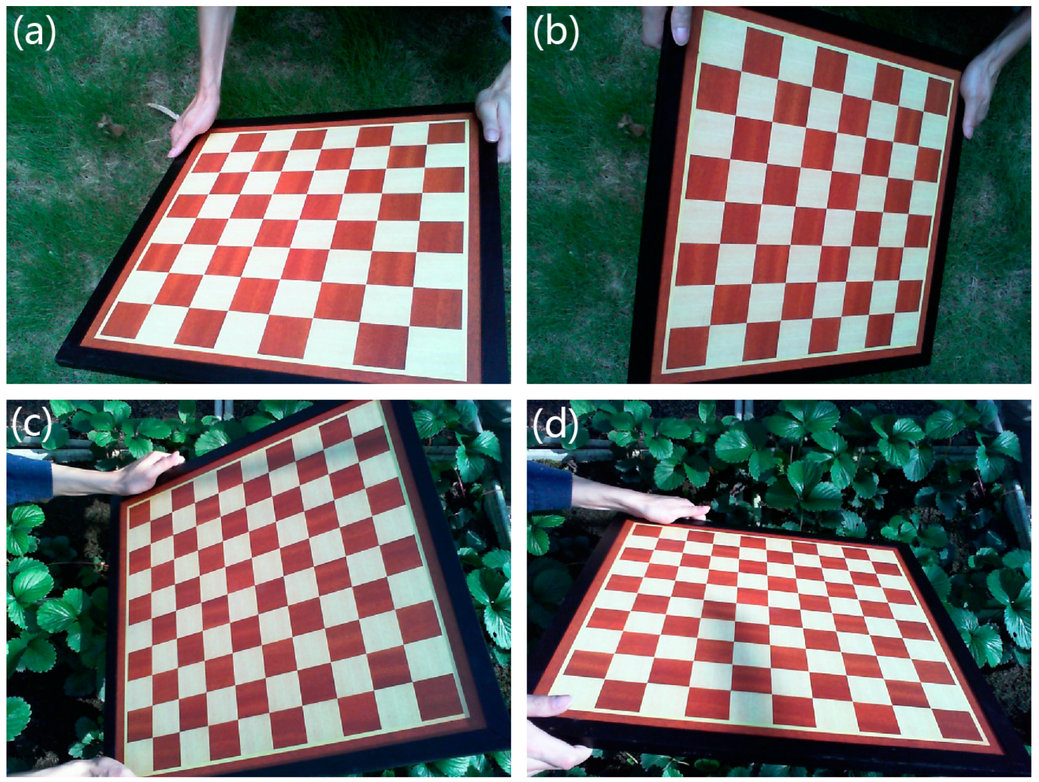
Figure 7.
A rectified image pair of a greenhouse ornamental plant.

Figure 8.
The census measure for two pixels.

Figure 9.
Experimental results on the Middlebury datasets [48]. (a): ground truth images. (b–e): disparity images of proposed method, original ASW [39], GC [37], and SGBM [38], respectively. The algorithm can be considered a good one if it has a result similar to the ground truth. The proposed results are superior to the others.
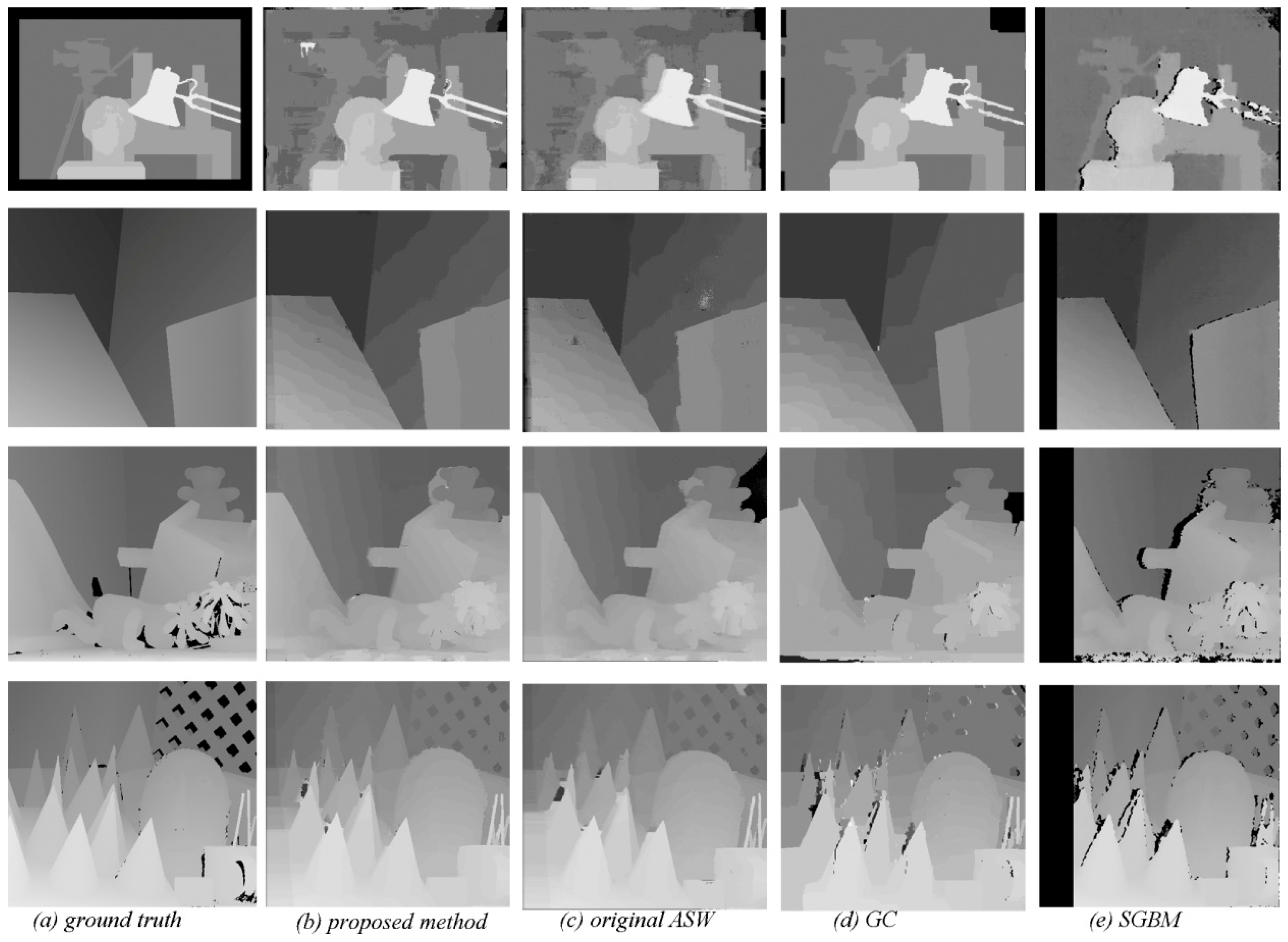
Figure 10.
Disparity images on real plant images: (a) real plant images; (b) disparity images generated by original ASW; (c) disparity images generated by the proposed method.
Figure 10.
Disparity images on real plant images: (a) real plant images; (b) disparity images generated by original ASW; (c) disparity images generated by the proposed method.

Figure 11.
Disparity maps and point clouds generated under four different baseline lengths: 45 mm, 65 mm, 85 mm, and 105 mm; the plant is placed about 1.0 meter away from the stereo system. (a) Disparity maps; (b) 3D point clouds viewed from the top of the plant; (c) ide-view point clouds, where each horizontal line stands for a depth layer; (d) the point clouds viewed from another viewpoint.

Figure 12.
Comparison of 3D point clouds of Epipremnum aureum obtained with and without disparity refinement: (a) the point cloud without disparity refinement; (b) the point cloud with disparity refinement.
Figure 12.
Comparison of 3D point clouds of Epipremnum aureum obtained with and without disparity refinement: (a) the point cloud without disparity refinement; (b) the point cloud with disparity refinement.

Figure 13.
The stereo-rectified left image and reconstructed 3D point cloud of the Epipremnum aureum sample plant. (a) The rectified left webcam image used for generating the 3D point cloud; (b,c) the reconstructed 3D point cloud of the Epipremnum aureum sample plant viewed from two different positions.

Figure 14.
The stereo-rectified left image and reconstructed 3D point cloud of the pepper sample plant. The left side (a) is the rectified left webcam image used for generating the 3D point cloud; (b) and (c) show the reconstructed 3D point cloud of the pepper sample plant viewed from two different positions.

Figure 15.
The stereo-rectified left image and reconstructed 3D point cloud of a Monstera deliciosa sample plant. The left side (a) is the rectified left webcam image used for generating the 3D point cloud; (b,c) show the reconstructed 3D point cloud of the Monstera deliciosa sample plant viewed from two different positions.

Figure 16.
The stereo-rectified left image and reconstructed 3D point cloud of greenhouse strawberry samples. The left side (a) is the rectified left webcam image used for generating the 3D point cloud; (b,c) show the reconstructed 3D point cloud of the strawberry sample plants viewed from two different positions.
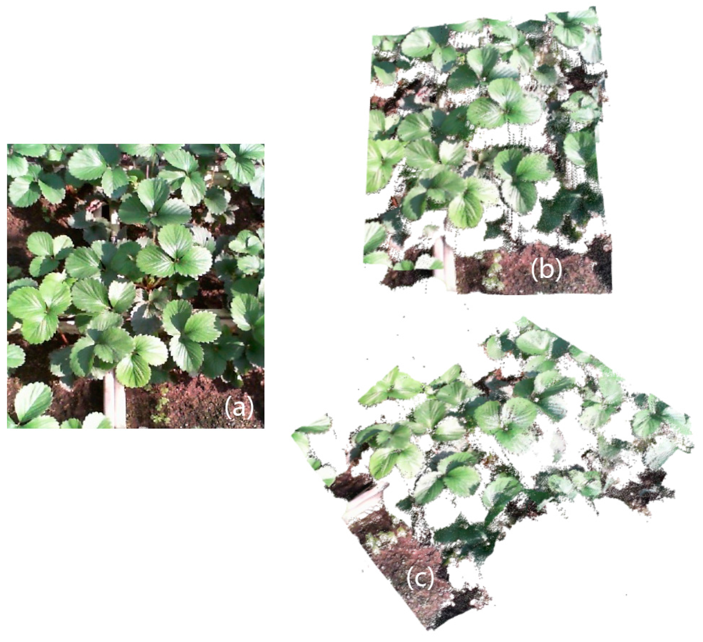
Figure 17.
The stereo-rectified left image and reconstructed 3D point cloud of greenhouse turnip samples. The left side (a) is the rectified left webcam image used for generating the 3D point cloud; (b,c) display the reconstructed 3D point cloud of the turnip sample plants viewed from two different positions.
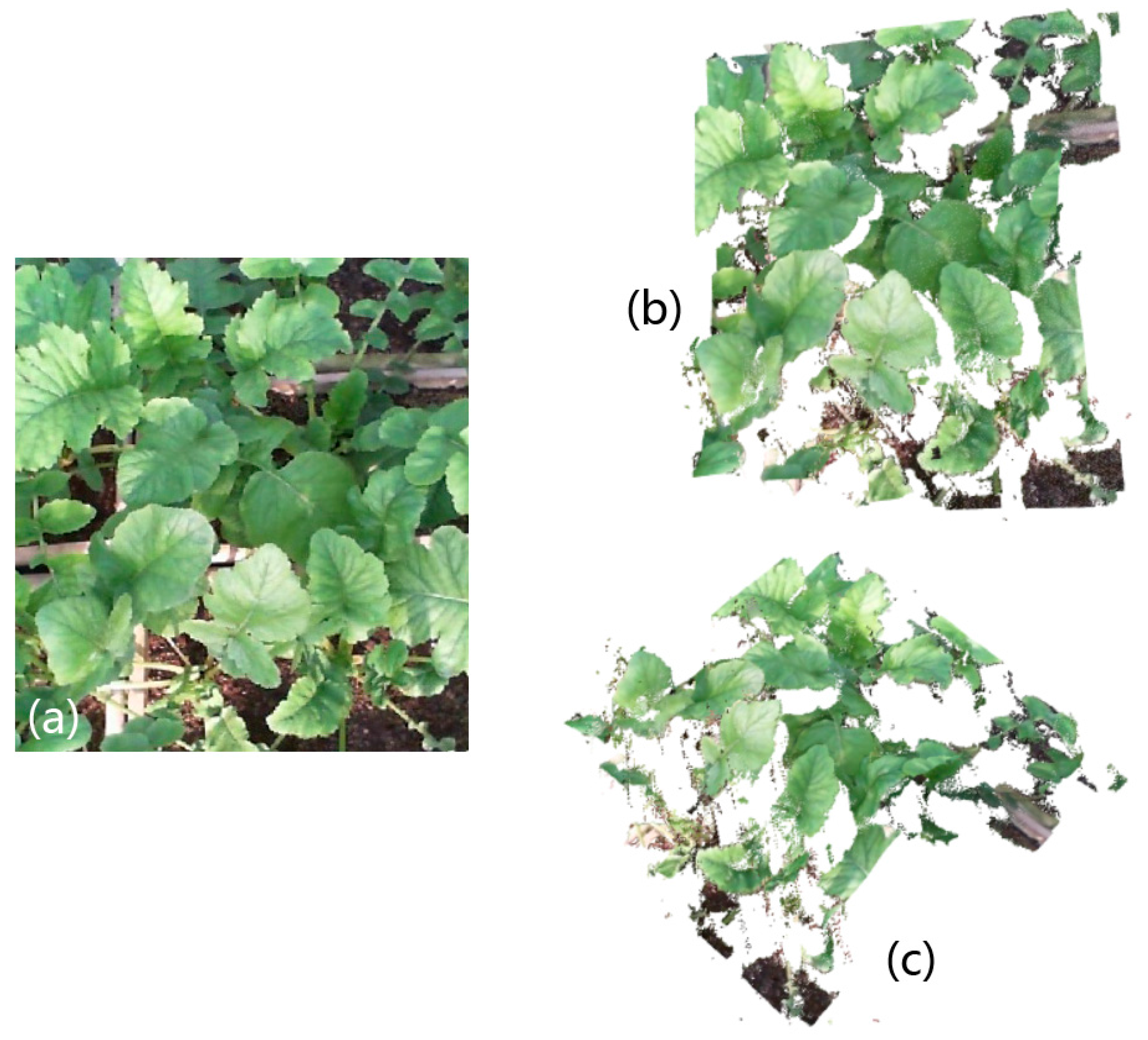
Figure 18.
A textured box was placed at different distances to the stereo platform for depth error measurements. The black number below each sub-image means the real distance from the box to the camera, and the red number below each box image means the measured depth error. The baseline of this test is fixed at 85 mm. It is noted that the absolute values of measured depth errors are also plotted as square data labels on the blue curve in Figure 19.

Figure 19.
Measured depth errors and the theoretical upper bounds in our stereo vision system. Each measured depth error is smaller than the corresponding upper bound value estimated by Equation (21).
Figure 19.
Measured depth errors and the theoretical upper bounds in our stereo vision system. Each measured depth error is smaller than the corresponding upper bound value estimated by Equation (21).

Figure 20.
Comparison of results in overcast and sunny weather for greenhouse strawberry plants: (a) the image captured when it is sunny; (b) the disparity image of (a) obtained via our ASW stereo matching algorithm with AD-Census cost measure; (c) the top view of the generated point cloud with disparity refinement on image (b); (d) the side view of the point cloud (c), from which we can observe the leaves distributed on different layers in height; (e) the image captured in overcast weather; (f) the disparity image of (e); (g) the top view of a generated point cloud with disparity refinement on image (f); (h) the side view of the point cloud (g), whose structure is almost the same as (d).
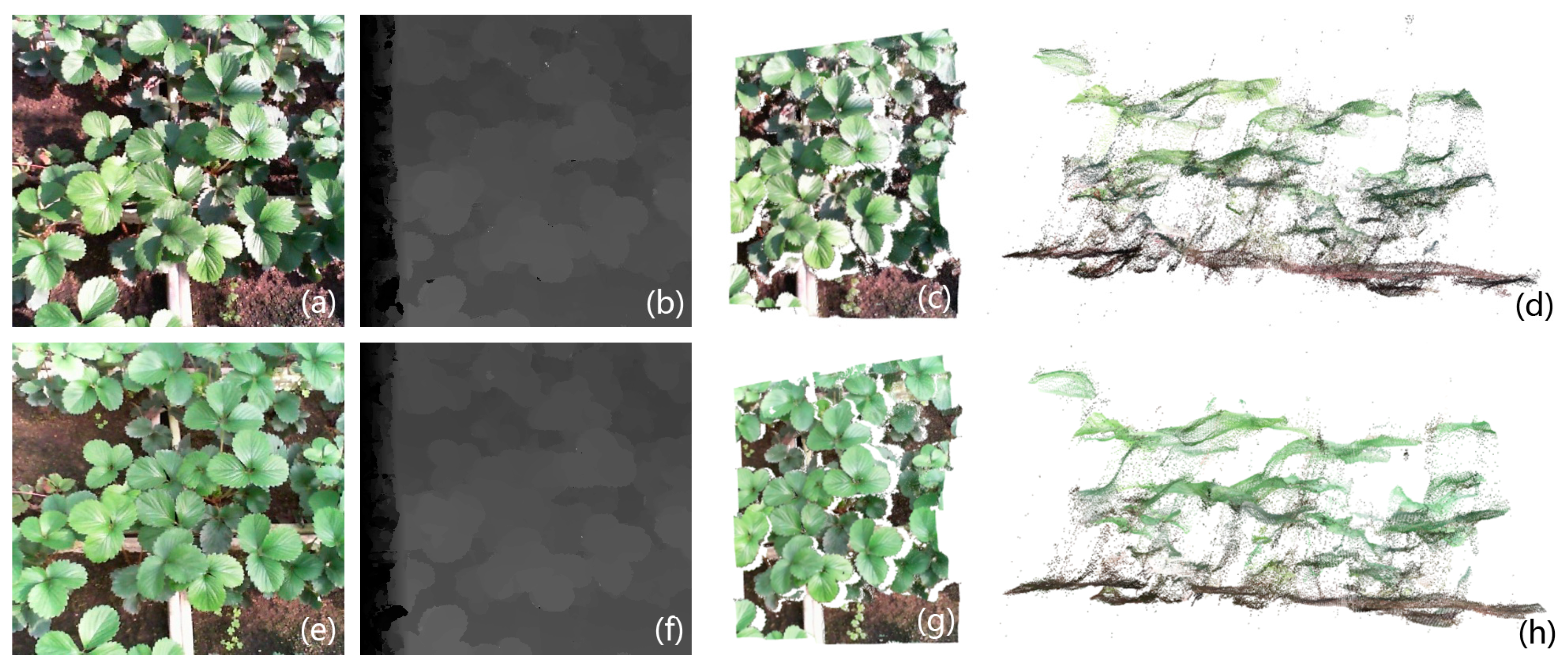
Figure 21.
Comparison of results in overcast and sunny weather for greenhouse turnip plants: (a) the image captured when it is overcast; (b) the disparity image of (a) obtained via our ASW stereo matching algorithm with AD-Census cost measure; (c) the top view of the generated point cloud with disparity refinement on image (b); (d) the side view of point cloud (c); (e) the image captured when sunny; (f) the disparity image of (e); (g)is the top view of the generated point cloud with disparity refinement on image (f); (h) the side view of the point cloud (g), with a structure almost the same as (d).
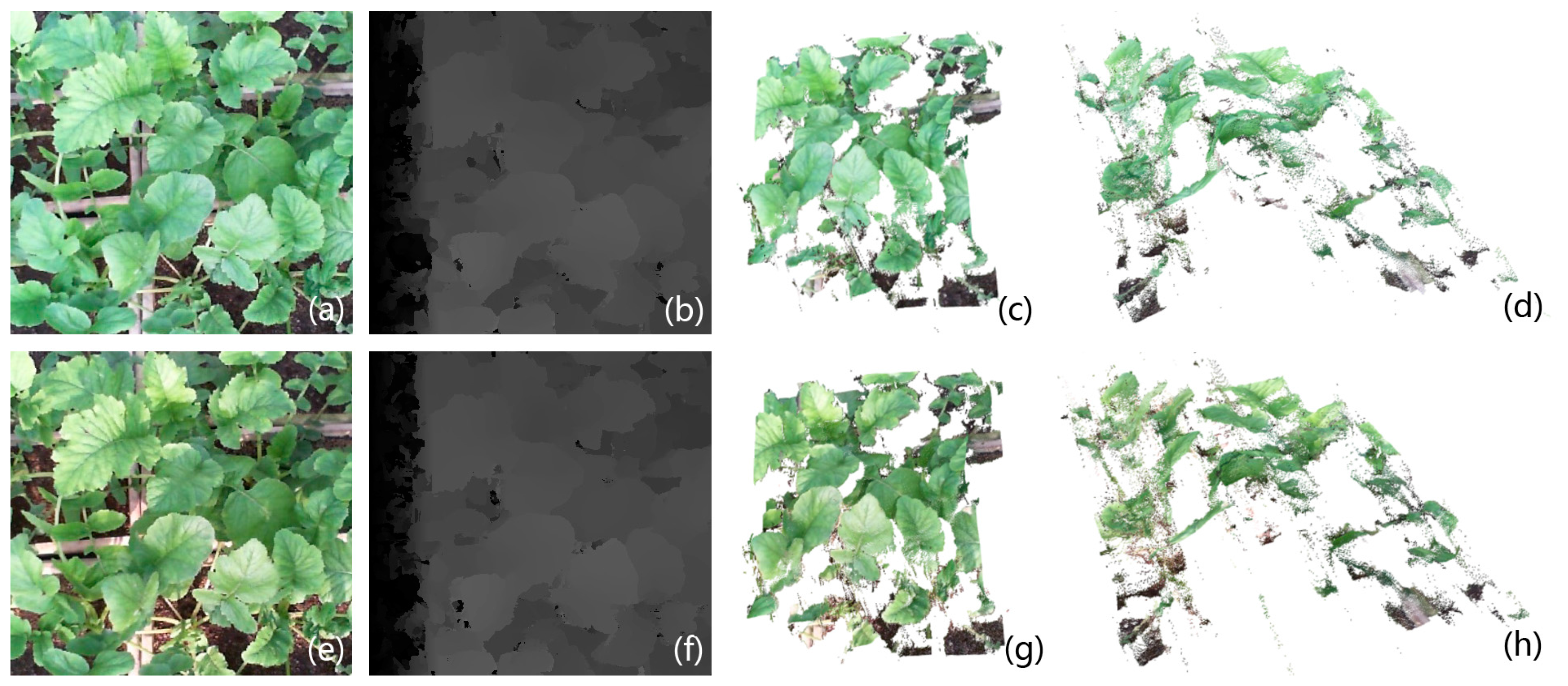
Figure 22.
Outdoor experiment on imaging a Monstera deliciosa sample plant: (a) image of the captured image pair, where the highlighted regions are labeled by red ellipses; (b) the disparity image of (a) obtained via our ASW stereo matching algorithm with the AD-Census cost measure. The disparity image exhibits invariance against highlight because there is no abrupt intensity change inside the highlight regions in (b). The two views of point cloud are shown in (c,d). The regions without highlight are mostly rugged, coinciding with the fact that highlight only comes from smooth and flat surfaces.

Figure 23.
Automatic leaf segmentation for the point cloud of the Epipremnum aureum sample plant. The point cloud contains the canopy structure only, and is obtained by using a green color filter on the original point cloud (Figure 13) generated by our method. (a,b) The side view and top view of the plant, respectively; (c,d) the segmentation results corresponding to (a,b), respectively. Different leaves are painted with different colors, and the points that are believed to belong to the same leaf are painted with the same color. The segmentation shows satisfactory performance, recognizing 35 of the 37 true leaves.

Table 1.
Comparison of the proposed method with the above approaches. Tsukuba, Venus, Teddy, and Cone are image pairs of the Middlebury datasets [48]. “n.o.”, “all”, and “dis” denote the mismatch rates for pixels in non-occluded regions, all pixels, and pixels near depth discontinuities, respectively. “Avg. Error” is the average error defined on Middlebury datasets. The best results are in bold face, and the proposed method achieves the best results at most times.
Tsukuba | Venus | Teddy | Cone | Avg. Error | |
|---|---|---|---|---|---|
| Unit: % | n.o. all dis | n.o. all dis | n.o. all dis | n.o. all dis | |
| Proposed | 2.45 3.53 6.58 | 0.38 1.09 4.39 | 6.97 10.7 18.9 | 2.91 11.6 8.75 | 6.63 |
| ASW [39] | 1.38 1.85 6.90 | 0.71 1.19 6.13 | 7.88 13.3 18.6 | 3.97 9.79 8.26 | 6.67 |
| GC [37] | 1.94 4.12 9.39 | 1.79 3.44 8.75 | 16.5 25.0 24.9 | 7.70 18.2 15.3 | 11.4 |
| SGBM [38] | 4.36 6.47 18.8 | 5.90 7.52 26.3 | 15.5 24.2 26.9 | 12.2 22.1 20.4 | 15.9 |
Table 2.
Implementation details about each step of the proposed 3D imaging method. The information listed here includes the software, equipment, URLs for tools, processing time, and data description.
Table 2.
Implementation details about each step of the proposed 3D imaging method. The information listed here includes the software, equipment, URLs for tools, processing time, and data description.
| Steps: | Image Acquisition | Calibration | Rectification | Stereo Matching | 3D Reconstruction and Display |
|---|---|---|---|---|---|
| Software/Equipment | VS2010+OPENCV2.4.9/The proposed platform | Matlab2014a/Laptop | VS2010+OPENCV2.4.9/Laptop | VS2010+OPENCV2.4.9/Laptop | VS2013+PCL1.7.2 (×86)/Laptop |
| URLs | Microsoft.com; Opencv.org | Vision.caltech.edu/bouguetj/calib_doc/ | Microsoft.com; Opencv.org | Microsoft.com; Opencv.org | Microsoft.com; Pointclouds.org |
| Time (minute) | Less than 3 | About 20 | Less than 1 | Less than 2 | Less than 1 |
| Data size | 40 + 2 images | 40 images | 2 images | 1 scene (point cloud) | 1 scene (point cloud) |
© 2017 by the authors. Licensee MDPI, Basel, Switzerland. This article is an open access article distributed under the terms and conditions of the Creative Commons Attribution (CC BY) license (http://creativecommons.org/licenses/by/4.0/).
Share and Cite
MDPI and ACS Style
Li, D.; Xu, L.; Tang, X.-s.; Sun, S.; Cai, X.; Zhang, P. 3D Imaging of Greenhouse Plants with an Inexpensive Binocular Stereo Vision System. Remote Sens. 2017, 9, 508. https://doi.org/10.3390/rs9050508
AMA Style
Li D, Xu L, Tang X-s, Sun S, Cai X, Zhang P. 3D Imaging of Greenhouse Plants with an Inexpensive Binocular Stereo Vision System. Remote Sensing. 2017; 9(5):508. https://doi.org/10.3390/rs9050508
Chicago/Turabian StyleLi, Dawei, Lihong Xu, Xue-song Tang, Shaoyuan Sun, Xin Cai, and Peng Zhang. 2017. "3D Imaging of Greenhouse Plants with an Inexpensive Binocular Stereo Vision System" Remote Sensing 9, no. 5: 508. https://doi.org/10.3390/rs9050508
Note that from the first issue of 2016, this journal uses article numbers instead of page numbers. See further details here.