Article

A Broad-Area Method for the Diurnal Characterisation of Upwelling Medium Wave Infrared Radiation

1
School of Science, RMIT University, Melbourne 3000, Australia
2
Bushfire and Natural Hazards Co-operative Research Centre, Melbourne 3000, Australia
3
Faculty for Geo-Information Science and Earth Observation (ITC), University of Twente, Enschede 7500AA, The Netherlands
*
Author to whom correspondence should be addressed.
Remote Sens. 2017, 9(2), 167; https://doi.org/10.3390/rs9020167
Submission received: 15 December 2016 / Revised: 9 February 2017 / Accepted: 13 February 2017 / Published: 17 February 2017

Abstract

:
Fire detection from satellite sensors relies on an accurate estimation of the unperturbed state of a target pixel, from which an anomaly can be isolated. Methods for estimating the radiation budget of a pixel without fire depend upon training data derived from the location’s recent history of brightness temperature variation over the diurnal cycle, which can be vulnerable to cloud contamination and the effects of weather. This study proposes a new method that utilises the common solar budget found at a given latitude in conjunction with an area’s local solar time to aggregate a broad-area training dataset, which can be used to model the expected diurnal temperature cycle of a location. This training data is then used in a temperature fitting process with the measured brightness temperatures in a pixel, and compared to pixel-derived training data and contextual methods of background temperature determination. Results of this study show similar accuracy between clear-sky medium wave infrared upwelling radiation and the diurnal temperature cycle estimation compared to previous methods, with demonstrable improvements in processing time and training data availability. This method can be used in conjunction with brightness temperature thresholds to provide a baseline for upwelling radiation, from which positive thermal anomalies such as fire can be isolated.

Graphical Abstract

1. Introduction

Active fire in the landscape is a major catalyst for environmental change, potentially resulting in large socio-economic impacts, including the high costs and risks associated with mitigation efforts and the disruptive evacuation of communities [1]. Fire authorities and land managers are constantly seeking new techniques for the early detection of fire to assist in the timely informing and evacuation of the public from at-risk areas, the planning and prioritisation of asset management strategies, and feasibility assessment of possible suppression efforts. This requirement for active fire detection in near real-time has seen the adoption of remote sensing from satellite sensors as an objective means to quantify and characterise the location, spread and intensity of fire events to support these important decisions [2]. The information derived from this imagery can also be used in conjunction with other data to provide models of an event, leading to more accurate understanding of the potential impacts of an event before they occur.
Remote sensing for fire detection and attribution has predominantly focused on imagery from low earth orbiting (LEO) sensors, which have significant advantages with regard to spatial resolution, and therefore to the minimum size of fire that can be detected. The trade-off with sensors of this type is that their orbital parameters preclude rapidly repeated observations of a single location, and without a significant investment in capital to provide for more missions, the ability to provide real-time observations of fire from these sensors will be hampered by extensive revisit times. The necessity for rapid fire detection sees the focus of fire detection shift to imagery obtained from geostationary sensors, which provide an increased revisit rate at the cost of a loss of fidelity in the spatial and radiometric realms [3]. Despite this, the launch of new sensors such as the Japanese Meteorological Agency’s Advanced Himawai Imager (AHI) and the NOAA’s Advanced Baseline Imager (ABI) provide an enhanced opportunity to examine fire ignitions and evolution due to improved spatial, radiometric and temporal resolutions compared to their geostationary predecessors.
One of the physical limitations of some techniques used for the remote sensing of fire is determination of the background temperature of a pixel. Having an accurate measure of this temperature is vital in order to be able to classify a target pixel as containing a fire in the first place, along with being able to accurately estimate the area of the pixel containing fire and the intensity or radiative output of the fire [2]. Background temperature tends to be a difficult value to determine accurately because of the obscuring effects of the fire’s output, which outweighs the background signal from a pixel in the medium wave infrared. Early efforts to correct for this behaviour used a bi-spectral approach [4], which used the response of thermal infrared bands in the same area to develop an estimate of fire characteristics. Thermal infrared bands also display sensitivity to fire outputs but to a much lesser extent and are generally used for false alarm detection, especially for marginal detections from the medium wave infrared caused by solar reflection [5]. The difference between signal response in these two bands is the basis for most current geostationary fire detection algorithms and similarly with the analysis of LEO sensor data [2]. Issues with these algorithms start when looking at fires of smaller extents. A study by Giglio and Kendall [6] highlighted issues with fire retrievals using the bi-spectral method, especially with regard to smaller fires and background temperature characterisation. The study found that misattribution of the background temperature by as little as 1 K for fires that covered a portion of a pixel ( p 0 . 0001 ) could produce errors in fire area attribution by a factor of 100 or more, with a less significant error in temperature retrieval of > ± 200 K. This is of major concern for the use of geostationary sensors for detection, as fires in their early stages make up far less a proportion of a pixel from a geostationary sensor than is the case with a LEO sensor.
The most common method of deriving background temperature for a fire pixel is through the use of brightness temperatures of pixels adjacent to the target pixel [2]. By identifying a number of pixels in the immediate area that are not affected by fire or other occlusion such as smoke and cloud, an estimate can be found by aggregation of the brightness temperature of these pixels. The assumption is made that the adjacent pixels used are of a similar nature in terms of reflectance and emissivity to the target pixel. This background characterisation is then used in comparison to the target pixel in order to identify whether the fire signal is different enough from the background to constitute a fire return. Problems occur with this method when the background temperature is misrepresented. In a study by Giglio and Schroeder [7] estimation of the background temperature from adjacent pixels in approximately 22% of cases produced a background temperature that was higher than the brightness temperature of the detected fire, based upon the surface variability of the area surrounding the detection. This study also analysed the general performance of the MODIS bi-spectral fire detection algorithm [8], and found that only 7% of the fire identified by the product could be accurately characterised for fire temperature and area. With the coarser spatial resolution of geostationary sensors, the authors noted that larger potential errors will affect the retrieval of fires in comparison to LEO sensors when using these methods.
A promising method for background temperature determination is through the use of time series data from geostationary sensors. This time series data can be utilised based upon the premise that upwelling radiation can be predicted based upon incident solar radiation, which varies chiefly by time of day, with some variation due to weather effects and occlusion. Modelling of this Diurnal Temperature Cycle (DTC) has been approached using many different techniques. Earlier work on the modelling of the DTC looked to provide a parameter-based description based upon fitting to discrete mathematical functions, such as the model proposed by Göttsche and Olesen [9]. This work applied the modelled DTC estimate directly to measured brightness temperatures using empirically derived parameters. This approach tended to be insensitive to functional variation due to synoptic effects, and performed inadequately during the period of rapid temperature change in the early morning. The work of van den Bergh and Frost [10] was the first to utilise a set of prior observations as training data for a signal fitting process, using the mean of previous observations as a state vector for a Kalman filter, which due to the sensitivity of a mean-based estimate to outlying observations, application was limited to cloud-free data only.
The influence of outliers on the training data used for signal fitting was addressed in part by the study of Roberts and Wooster [11], who looked at a selective process whereby previous days DTCs were included in the training data of a pixel based upon the amount of disturbance in the day’s observations, with a limit of six cloud or fire affected observations out of a 96 image DTC permitted. These limits eliminated much of the effects of outliers on the subsequent single value decomposition (SVD) used for the initial fitting of background temperature. Issues occurred in areas where there were insufficient anomaly-free days for a fitting to be performed, even with a sampling size of the previous thirty days, in which case DTCs were selected from a library of known anomaly-free DTCs from a similar area. The process was reliant on an accurate cloud mask to determine which days were anomaly-free, and the training data derivation was data intensive, with DTC vectors having to be extracted and calculated for each individual pixel prior to fitting using the SVD process. These issues lead to training data fragility, and introduced some of the issues that are common error sources in contextual algorithms for fire detection.
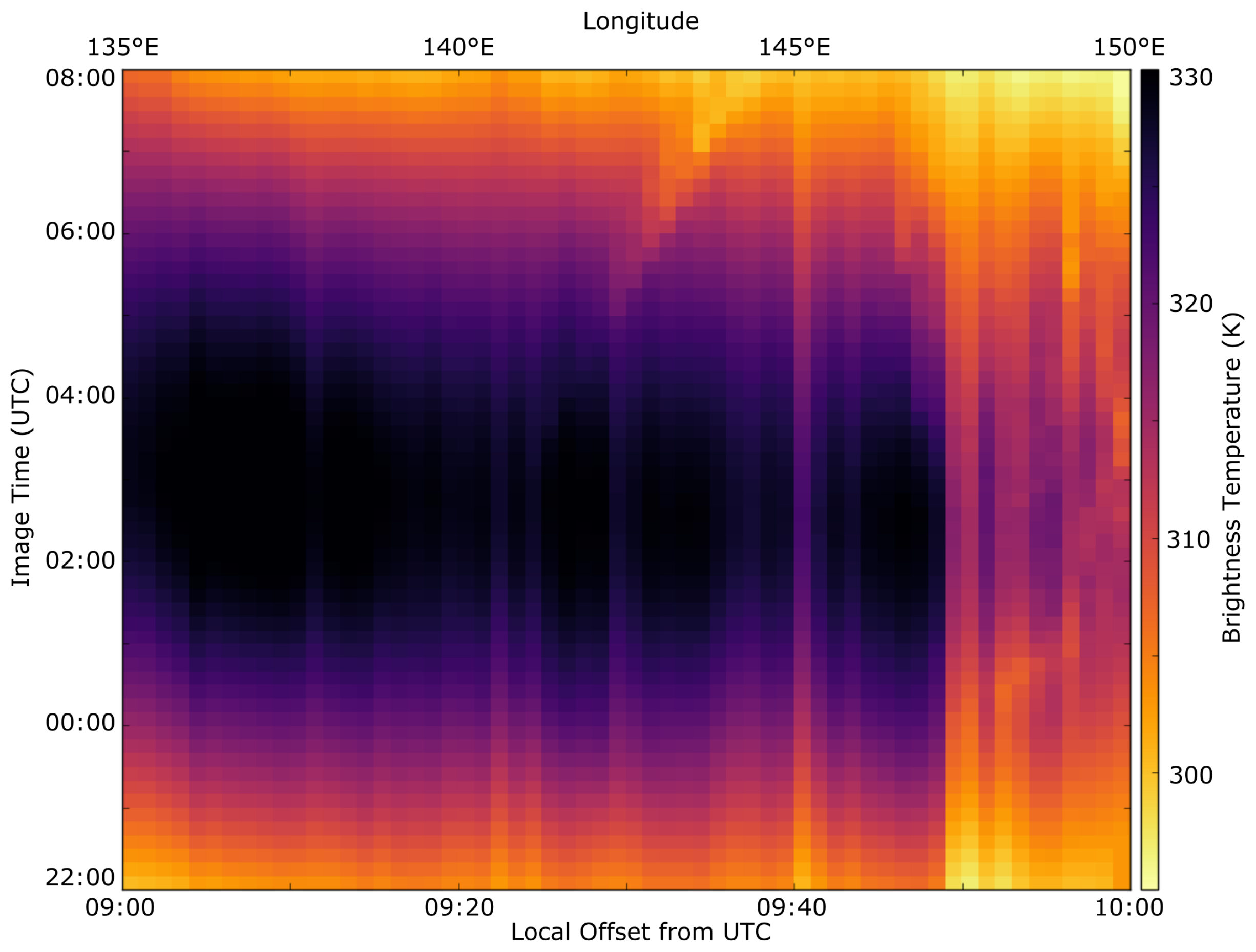
In order to address the issues caused by sampling training data from a pixel-based approach, this paper presents a new method for deriving training data based upon a broad-area method. This method exploits similarities in incident solar radiation found at similar latitudes to derive training data for a pixel. Geostationary sensor data is aggregated by latitude and an area’s local solar time, and formed into a time series based upon a sensor’s temporal resolution. This paper will compare the results obtained using this method to training data derived from individual pixels, such as in the study by Roberts and Wooster [11], and with contextual methods of background temperature determination, to compare the accuracy, efficiency and availability of each method.

2. Materials and Methods

2.1. Himawari AHI-8 Data

The Japanese Meteorological Agency (JMA) launched the Himawari-8 geostationary satellite in October 2014, which replaced the MTSAT-2 sensor as the main source of meteorological data for Australia. The sensor onboard the Himawari-8 satellite is the Advanced Himawari Imager (AHI), a sensor capable of measuring 16 bands of imagery, ranging from visible light through to thermal infrared. The radiometric resolution of the sensor is significantly improved compared to previous iterations of MT-SAT, with quantization of 11 bit in the visible and near infra-red and up to 14 bits for the MWIR Band 7, which is the band most heavily utilised for fire detection purposes. The sensor boasts a spatial resolution of 2 × 2 km at nadir for infra-red channels, with visible imagery available at resolutions as high as 0.5 × 0.5 km. Scanning of the full disk generally takes place every ten minutes, with the area of Japan and surroundings scanned every 150 seconds. The coverage area of images provided by the sensor ranges from western India to Hawaii longitudinally, encompassing much of China, Siberia, Japan, South East Asia, Indonesia and Australia. Characteristics of AHI and MTSAT-2 for fire detection can be found in Table 1.
The increase in image frequency from the AHI sensor in particular allows for greater utilisation of time series data for temperature estimation, with gaps in the data caused by station keeping, or sensor recording and processing issues having less of an effect on derived values. Improvements in radiometric resolution allow a greater range of measurements to be recorded, improving the fidelity of anomaly detection, and a greater saturation temperature allows for the characteristics of larger fires to be determined. Preliminary work with this sensor in the fire detection space [12,13] has demonstrated the ability to detect and track fires using multiple bands of imagery from this satellite sensor.
Inclusive of the housekeeping periods of the satellite, which occur twice daily, 142 full disk images are available from AHI per day. This study utilises image products published by the Australian Bureau of Meteorology (ABOM), derived from raw AHI images by the process outlined in [14] for Band 7 brightness temperature corrections from raw satellite imagery. The study also makes use of the clear sky probability product, adapted by ABOM from the CLAVR-x cloud mask algorithm outlined in Heidinger [15] with some minor alterations [16] for verification of cloudy periods in the temporal data stream. Cloud product data for AHI is generally available at ten minute intervals, which is similar to raw satellite images.

2.2. Training Data Derivation

Upwelling radiation in the medium wave infra-red consists of two main components: reflection of solar radiation from the earth’s surface, and emission of blackbody radiation from the surface due to temperature. The skin surface temperature of the earth is influenced by a number of factors. Rain reduces upwelling radiation by both lowering surface albedo, and reducing surface temperatures and consequently emission. Convective cooling and heating due to air masses can influence surface temperatures, and land cover composition can affect the magnitude of temperature change. However, the most notable influence is heating by solar radiation. For any area of land on a given day at a given latitude, the amount of incident solar radiation should be similar barring obscuration. This should lead to a similar relative diurnal response of upwelling radiation from the land surface at a given solar time t s . By breaking the land surface into 0.25°× 0.25° blocks, we can use the rotation of the earth to construct an amalgamated time series, with each block translating to a separate minute of local solar time.
Images from the sensor have an ocean mask and a rudimentary cloud mask (all pixels below 270 K discarded) applied, and the remaining pixels in each block are aggregated as a median brightness temperature. This swath of blocks from a latitude is assigned a time according to the UTC time of the image capture and the longitude of the block as a function of its offset from the Greenwich meridian:
t s = U T C i m a g e + l o n g i t u d e × 240 ( s e c s )
Each line of the original image also has a scan line time associated with it, which is the offset of the line capture relative to the nominal image time. This is important, especially when comparing areas of relative spatial proximity that may be scanned at different times in the image capture cycle. Blocks are assigned their own scan line time according to the median scan time of the captured pixels from the original image. Once this is added, each block’s apparent time is rounded to the nearest minute and training data processing can commence.
An example of the variability in training data can be found in Figure 1, which is a swath of land running half the width of the Australian continent at 26°S latitude. This swath demonstrates the diurnal variation of the daytime period of each block as the image time advances. The timing of the peak temperature of the day advances from right to left as the images progress, which should be the expected behaviour as the Earth rotates. Most noticeable in this figure is the differing magnitude of temperature changes in the most easterly three degrees of longitude. In this region the land cover changes from the sparsely vegetated desert found in central Australia to more vegetated cropping land interspersed with forest. This composition of land cover displays far less upwelling radiation during the middle of the day than much of the rest of the swath, necessitating the step of temperature standardisation for each block to account for this reduced range of radiation values.
Figure 2 shows the relationship of the swath to local solar time as time passes. Each of the grey lines on this graph represents median brightness temperatures relative to local solar time for each block. The coloured lines represent the temperature trajectories of a selection of blocks from the swath. In an ideal situation these lines would sit on top of one another, but variations in land cover and partial obscuration of blocks by cloud, especially on the most easterly vector depicted in green, have prevented it in this instance. Nonetheless, the daily maximums of the other trajectories occur almost at the same point, between 12:30 and 13:00 local time. One characteristic this diagram demonstrates is the overlapping redundant information available in the ten minute time series provided by the AHI sensor. Swaths of sufficient width produce large amounts of redundant measurements at each local solar time depending on the imaging frequency of the satellite sensor in question.
Both Figure 1 and Figure 2 demonstrate a basic issue with this block aggregation method, which is the variation of responses from the land surface in each block due to factors such as differences in surface emissivity and reflection, and the influence of cloud shadowing. In order to minimise the effects of this over the time series, each of the blocks is standardised (mean μ = 0, standard deviation σ = 1) over a 24-h period and these standardised values are used in the signal generation process. The data is then merged into one large time series and medians of the deviation from the daily mean of each block are taken at each minute. This information is then fed through a Butterworth low pass filter (fifth order, cutoff frequency three hours) to smooth some of the minute-to-minute variation and provide an ideal temperature curve for the day in question. The result of an example of this process is shown as the red line in Figure 3. This filtered data subsequently forms the Broad Area Training (BAT) data set for the fitting of a diurnal temperature curve to the target pixel.

2.3. Fitting to Pixel Brightness Temperatures

This study makes use of the robust matching algorithm described in Roberts and Wooster [11], which adapted the SVD method described by Black and Jepson [17] for its fitting method. In a similar fashion to the training data set, each pixel brightness temperature value in the 24-h period to be modelled is categorised by local solar time. These times are rounded to the nearest minute to more easily correspond with the training dataset. The time offset between the first brightness temperature measurement of the pixel and the training data is calculated, and the values are extracted from the training dataset corresponding to the image times of the pixel dataset. This leaves the training dataset consisting of a number of daily vectors that correspond directly to the times that brightness temperatures were measured for the pixel’s DTC.
A SVD decomposes the training data matrix A into a number of principal component vectors U which describe the training data as a series of orthogonal vectors, along with the diagonal matrix Σ which contains sorted decreasing eigenvalues for each component and the matrix V which contains coefficients for the reconstruction of the basis DTCs, as shown in Equation (2):
A = U Σ V T
Given the datasets involved with the brightness temperature fitting process used in this paper, a significant number of the component vectors in U contribute little to the DTC fitting process. An examination of the relationship between the maximum variance in the training data and the DTC is given by the eigenvalues σ i found in Σ. To minimise the effect of overfitting caused by these extra degrees of freedom in the component vectors, values of σ i are tallied until the examined eigenvectors account for at least 90% of the total variance of the SVD (per Rajaraman and Ullman [18]), with subsequent vectors discarded. This generally leads to a U matrix consisting of between two and seven vectors for fitting in this study.
For a vector of observations from a pixel e, an approximation of the DTC e * can be created from a reconstruction of the principal components:
e * = i = 1 K c i U i t
where K is the number of basis vectors used and c i is a series of scalar values derived by taking the inner product of the observations from the pixel and the principal components ( e T U ). c i essentially describes the contribution of each of the component vectors in U to the fitted estimate of the DTC e * .
At this point, the root mean square difference of the estimate of the DTC is compared to the raw temperature measurements. If there is a sufficient fit between the two at this point, the model answer is accepted without adjustment. If not, to minimise the effects of outliers on the robust determination of the DTC, a least squares minimisation of Equation (3) occurs, utilising a robust error norm which identifies outliers that contribute excessively to error:
σ ( x , s ) = x 2 s + x 2
x is the value of e - e * at time t, and s is a scale factor which can be reduced iteratively to improve the solution given by the error minimisation. Care should be taken when selecting suitable s values to ensure appropriate outlier elimination and that the model does not become unstable. This leads to the application of an outlier mask m, such that:
m t = 1 , | e t - e t * | σ / 3 0 , o t h e r w i s e
which leads to the minimisation of the error function E ( c ) as shown below:
E ( c ) = t = 1 N m t ρ ( ( e t - ( i = 1 K c i U i t ) ) , σ )
In a set of randomly selected DTCs, the number of anomalies produced by cloud far outweighs that of fire. In order to minimise the influence of sporadic clouds to the temperature fitting process and keep the modelled curve closer to higher temperatures that are more reflective of ground conditions, the weights of all negative residuals are halved during the least squares minimisation process.
This process refines the values of c i applied to the principal components U i in order to reconstruct an approximate value for e t . At this point, outliers from the ideal DTC can be identified and attributed according to their characteristics—whether they are positive or negative anomalies, and whether the change occurs suddenly or gradually over time.

2.4. Algorithm Evaluation

2.4.1. Method Accuracy

In order to test the accuracy of brightness temperature modelling using BAT data, a number of comparisons are made with currently used methods for deriving brightness temperature. Focus will be placed upon the method described by Roberts and Wooster [11], which gathers training data vectors from the pixel’s recent history, ranging up to thirty days prior to the time period being fitted. This method uses a rejection criteria based upon the number of pixel returns in a 24-h set affected by cloud, with rejection of a daily vector based upon more than 6.25% of pixel returns in the period being cloud-affected (six of the 96 images available). A pixel can be classed as able to be modelled using this training data if at least ten days out of the previous thirty are classified as successful and only successful vectors are utilised in the SVD fitting process. A similar process is used to apply this method to pixel history in this study, with a small alteration in the number of bad pixels causing a rejection. As the AHI sensor takes a maximum of 142 images in a 24 hr period, a rejection of a daily vector occurs when there are more than nine instances of clear sky probability equal to zero in the corresponding AHI cloud mask data.
For comparison, a temperature fitting has been applied to each sampled pixel utilising BAT data derived from the previous thirty days and the previous ten days prior to the fitting. These sampling points simulate the minimum and maximum amount of training data available to the pixel-based fitting approach. Comparison is also made to contextual based temperature derivation based upon a similar method used for the MODIS fire products [19], with an expanding kernel based upon 25% cloud and fire-free returns in the target vicinity, with a minimum of six successful returns. In the case of the MODIS products, the kernel is allowed to grow to 21 × 21 pixels in size before reaching a failed state. Due to the larger areas covered by AHI pixels, the divergence of land cover and geology over these distances could be extreme, so a limit of 5 × 5 pixels was proposed instead. For this evaluation, a set of 19,916 pixels were randomly selected over the Australian continent for the month of November 2015, with fitting of the raw brightness temperature performed using the four different methods noted above.

2.4.2. Method Efficiency

The nature of the BAT method lends itself to pre-processing—once a swath has processed from a particular image time, the data is utilised in any fitting process on any pixel in the swath for the encompassing period (either ten or thirty days in the case of this study). For each image, an ocean mask and basic cloud mask (such as described in Section 2.2) is applied before blocks are aggregated by median temperature. This data is stored in files for later access in the block-based fitting method.
For evaluation of the efficiency of both algorithms, the Python code for both methods was written to take advantage of an initial common data gathering process (location, start time, daily brightness temperature, available cloud). A random location and time in Australia during the month of November 2015 was selected, with the pixel-based training data calculated first. An extraction routine for training data was run once the suitability of an individual day of data was assessed. This routine would then check whether sufficient training periods for a pixel existed, and ran the fitting routine in the event of success. The time taken for both successful and unsuccessful routines using pixel-based training data was recorded.
Next, the BAT fitting was undertaken using thirty training days and ten training days, utilising the pre-processed block data, with the processing time for each recorded. Processing took place utilising code written for Python 2.7, using the Numpy (v1.12) mathematical processing module and the built-in multiprocessing module, along with the python-netCDF4 (v1.2.1) module for data reading and writing. The computer used for processing utilises an Intel(R) Core(TM) i7-5820K CPU, allowing 12 threads of processing to take place at once on the six available cores. Images and pre-processed training data were stored on and accessed from an external hard disk drive using USB-3 for data transfer.

2.4.3. Training Data Availability

In order to calculate the availability of pixel-based training data as per the [11] method, we used the AHI cloud mask data to evaluate cloud cover at the time of each image, with all values of clear sky probability greater than zero counting as clear sky. The data was aggregated for each pixel for a 24-h period corresponding with a UTC day, and pixels with greater than 132 cloud-free returns judged to be suitable for training purposes. Ten or more such successes within the thirty day period evaluated made the pixel suitable for pixel based training data collection. As the BAT datasets rely on redundant measurements from adjacent blocks on the swath—with a consequent reduction on reliance upon an individual block for training data—it was difficult to provide a direct comparison case back to the pixel-derived data for evaluating availability. Absences in measurements from a specific block lead to reductions in the accuracy of the training data model for the at-large swath, but complete loss of model performance only occurs where a significant length of an individual swath is completely obscured by cloud for an extended period, which is unlikely outside of situations where the swath is very narrow. For a comparison in this case, we used the availability of pixel training data on a per-pixel basis and the availability of BAT data on a per-block basis for the months of October and November 2015 for the Australian continent. The BAT availability figures in this case may be construed as a minimum, and effective training data availability is generally much higher.

3. Results

3.1. Algorithm Accuracy

For comparison purposes between the pixel-based and BAT methods, we processed solutions for a selection of 19,916 pixels with random locations on the Australian continent with fitting times during the month of November 2015. Of this larger selection, 5747 pixels (approximately 28.9%) had sufficient training data available for use of pixel-based fitting.
Table 2 shows the relative accuracy of each of the temperature fitting processes in comparison to the raw brightness temperatures recorded by the AHI sensor after measurements flagged as cloud are eliminated. In clear sky conditions (≤10 cloud instances) the pixel-based training method performed more accurately than the BAT method for either ten or thirty days of training data, with differences of 0.30 and 0.15 K respectively. This was expected, as the data derived from an individual pixel will perform far better with regard to localised effects on pixels such as land cover composition. As the number of cloud instances increased, the pixel-based training accuracy degraded, but the 30-day BAT method showed a steady relationship with the cloud free brightness temperatures up to 30 cloud affected returns, with a more gradual loss of accuracy on heavily cloud affected days. The 10-day BAT method showed a similar performance dynamic, with an approximate 20% loss in accuracy up to the point where accurate temperature determination became difficult (>50 clouds).
The context-based temperature derivation appears to perform especially well regardless of the number of outliers encountered in the temperature dataset. This is mainly due to the spatial autocorrelation of cloud and weather effects, which see contextual based temperatures closely track anomalous temperature as measured in each pixel, rather than tracking the base model of upwelling radiation without anomaly. Comparison is also inhibited by the instance of a contextual temperature not being available, which is more likely at times where anomalies would be detected.
Figure 4 demonstrates some examples of the fitting process over a few of the random pixels selected. Figure 4a shows the typical performance of each temperature estimation technique on a clear sky day, with the fitted curves from the BAT showing greatest variance from the raw temperatures during the night-time period and at the peak of the day. The pixel based training data is better able to handle tracking of brightness temperature during the daytime, but also shows some variance during the night to a lesser extent. Figure 4b shows an example of a day with between 20 and 30 cloud instances. This figure shows the fitting curves from both of the BAT datasets effectively ignoring the cloud induced anomalies in the early evening (0900 UTC) and during the peak of the following day (0200 UTC). This is in contrast to the pixel-based trained fitting, which follows the anomalies in the early evening more closely and underestimates the rising temperatures in the morning period (2000–0000 UTC). This figure also demonstrates the spatial autocorrelation issue with the contextually derived background temperatures. The contextual fitting follows the cloud affected temperatures in the afternoon and early evening period, ignoring the significance of the temperature peaks during this period which are more indicative of the true background temperature.
Figure 4c shows an example with around 95 instances of non-clear sky conditions. This example shows some of the fragility inherent in all of these methods when a significant portion of the DTC is cloud obscured. Due to the standardisation process that all pixels undertake before fitting of the training data is undertaken, the large temperature drops caused by the evening clouds (0700–1100) skew the normalisation by lowering the mean and increasing the standard deviation. This issue sees both the pixel-based fitting and the BAT fittings underestimate the background temperature throughout the course of the day, with the largest variations in the peak of the day and towards the end of the fitting in the early morning. This also demonstrates one of the limitations with using a model with greater degrees of freedom. Extra degrees of freedom are necessary in the case of sudden drops in the background temperature caused by weather effects, but on days where brightness temperatures do not follow the indicative shape of the DTC, the SVD fitting process tends to produce curves that wander about with little relation to the true background temperature.

3.2. Algorithm Efficiency

Table 3 shows the average time taken to perform the computations by each of the temperature fitting methods from a processed pool of 19,916 target pixels. The time taken to provide a temperature fitting based on BAT data for a thirty day period is approximately one-tenth of the time taken to derive a similar fitting from the pixel data. Part of the increase in speed comes from pre-processing of the pixel training data, which takes approximately 15 minutes per day of images. The difference between the pixel-based and block-based methods coincide at around 170 pixels evaluated, with the block-based method performing significantly faster beyond this. The pre-processed blocks can also be used in calculations for training data in adjacent time periods ±10 or 30 days from the start time of the original assessment, speeding up subsequent processing further. The largest improvement in time of processing between the two methods is with regard to acquiring data about the state of cloud in the training data period, where evaluating the suitability of 24-h periods using the cloud mask data makes up over 75% of the time taken to process a solution using this method.
The time taken to calculate a fitting from the 10-day BAT data is even shorter, taking around 40% as long as the thirty day BAT method. A significant improvement in processing time can be achieved for a small decrease in accuracy compared to the fitting provided by the 30-day BAT data. This is of importance in situations where processing time may be more critical than accuracy.

3.3. Training Data Availability

Training data blocks were derived for the entirety of the Australian continent for the months of October and November 2015, from 4379 and 4245 AHI Band 7 images respectively. Block method training data was deemed available when at least one pixel brightness temperature in a 0.25° block was observed above 270 K. Using the BAT method training data availability for the continent averaged 96.9% of all images for October and 95.4% of all images for November. This compared to the pixel-based method, which yielded 70.2% of data in October and 67.8% of data in November. Given the assumption that a minimum of ten days of training data is sufficient to derive a DTC, 91.4% of blocks demonstrate a sufficient number of clear days to derive training data in October, and 81.8% in November. In comparison the pixel based training method supplies sufficient days of training data to a pixel in 43.8% of cases in October and 37% of cases in November. From an availability standpoint, the block based method of training data derivation is a marked improvement over pixel-based methods, and a significant amount of redundant data on each line of blocks extends this availability further.
Figure 5 shows the spatial distribution of training data availability over the study area for October and November. The figure demonstrates the overall increase in training data availability when using the BAT method. Areas of limited availability demonstrated similarity in spatial distribution between the two methods, with south eastern Australia and Tasmania in particular suffering from a lack (indeed in some areas a total absence) of pixel-based training data for the evaluation period. In comparison, the majority of blocks retained availability for the required time during the period, with some deterioration in coastal areas. The BAT method demonstrates a significant improvement in temperature fitting ability, especially in the highly populated coastal areas in the south and east of Australia.

4. Discussion

The advantages of using the BAT method for deriving training data for temperature fitting include robustness against localised cloud, especially in areas with persistent standing cloud such as coasts and mountainous areas; the ability to minimise the number of training days required for deriving a brightness temperature fitting due to the increased availability of training data; and a reduction in the storage of data and processing time of training data for temperature fitting. Whilst in this study the training data is used to feed an SVD fitting of the DTC, the data could easily be applied to other fitting techniques, such as a random forest classifier or as a state vector for Kalman filtering. The nature of the fitting process removes the need for tracking locations that have standing hotspots, as the fitting process is completely context independent, and eliminates errors that may be caused by large variations in response to solar radiation and emission between adjacent pixels. As the broad area method relies on as few as one cloud-free pixel per block from which to derive a median temperature, the method is far more robust in response to occlusion than the pixel-based method. When banks of cloud associated with large weather systems are present, a single block may be totally covered by cloud in one or several images. However, the redundancy associated with evaluation on a continental scale means that this lack of data has a minimal effect on the training data for the same time period.
The quality of the training data used in the process relies on a couple of factors. For example, the width of the longitudinal swath at any given latitude is affected by the amount of ground available to sample that swath. In Australia, latitudes between 25°S–30°S have the full width of the continent to sample temperatures from, with anywhere up to 160 blocks of data per image. This provides a large amount of redundancy in the training data, reducing the affect of outliers in the training set. In contrast, a smaller swath width results in fewer blocks to formulate the training data, with a greater risk of anomalous returns affecting the resultant fitting processes. A smaller swath width also increases the influence of edge cases such as coastlines, which tend to moderate land surface temperature variance if they are not handled by an adequate ocean mask. A buffer of two pixels (between 3 and 6 km) was used to eliminate these edge cases for ocean boundaries, but water bodies such as lakes and reservoirs may also contribute to erroneous training data if the number of blocks used for training data is low. Discontinuous and inadequate areas to derive training data from may prove a challenge, and evaluating the performance of the BAT method in a region like Indonesia where cloud cover is high and land areas are discontinuous would properly test the limits of the method.
Deriving training data using the BAT method is not without its issues. The method involves the use of a median value for the entirety of a 0.25°× 0.25° block without taking into account factors such as land cover, land use type, slope and aspect, and surface emissivity, all variables that can vary significantly between pixels in a block. The application of the training data back to the pixel brightness temperature using the SVD process also omits consideration of differing albedo between adjacent pixels in a block. These issues may both be resolved by using a weight from each pixel at different times of the day to take into account the differing emissivity and reflection and how they affect the DTC of each location. The training dataset also has a minimum cutoff temperature of 270 K to minimise the influence of cloud affecting the training data in lieu of an operational cloud mask which may produce large areas of missing data in places where surface temperature and reflection components sit under this value for long periods of time. If a method such as this is used to track surface upwelling radiation in areas that have sustained brightness temperatures below 270 K, a cloud mask could be substituted in this case to eliminate major outlying temperatures instead. The effect of snow on brightness temperature tracking using this method has not been explored, mainly due to the study site and time of year chosen.
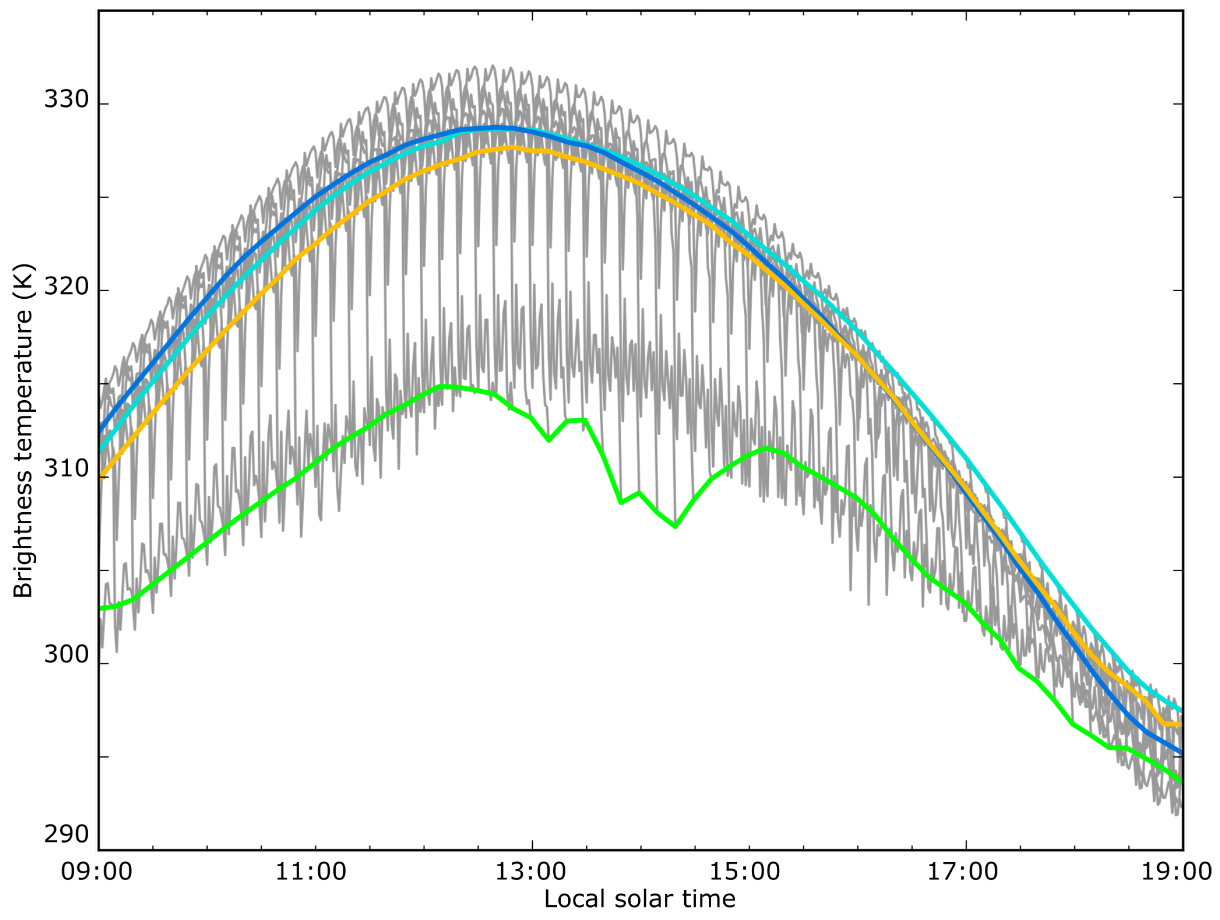
Considering the evaluation of the various methods for accuracy of fitting, the block-based training data based upon thirty previous days performed reasonably well for fitting accuracy in comparison to the pixel-based training data for all anomaly classifications, and the results derived from the 10-day block training data were of similar accuracy. If a threshold for suitability of fitting is placed on the results, such as would be for a fire detection model, the 30-day block-based method is far more robust with respect to anomalies and would continue tracking the expected upwelling radiation with up to one quarter of the time series obscured. A full sensitivity analysis using in-situ upwelling radiation data along with a verified cloud mask would be of value to confirm the shape of the diurnal model in order to provide an independent confirmation of the method’s accuracy. Of note here is the apparently extremely good performance of the contextual method for providing background temperature, which is an unfortunate side effect of methods for evaluating the accuracy of the model fitting process. The high spatial autocorrelation demonstrated by upwelling radiation results in a contextual based temperature tracking extremely closely to the raw temperature measurements regardless of whether the surrounds themselves are affected by anomalies such as cloud, smoke or fire.
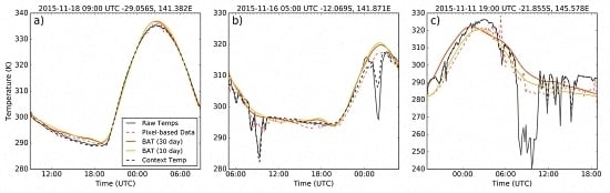
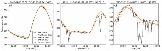
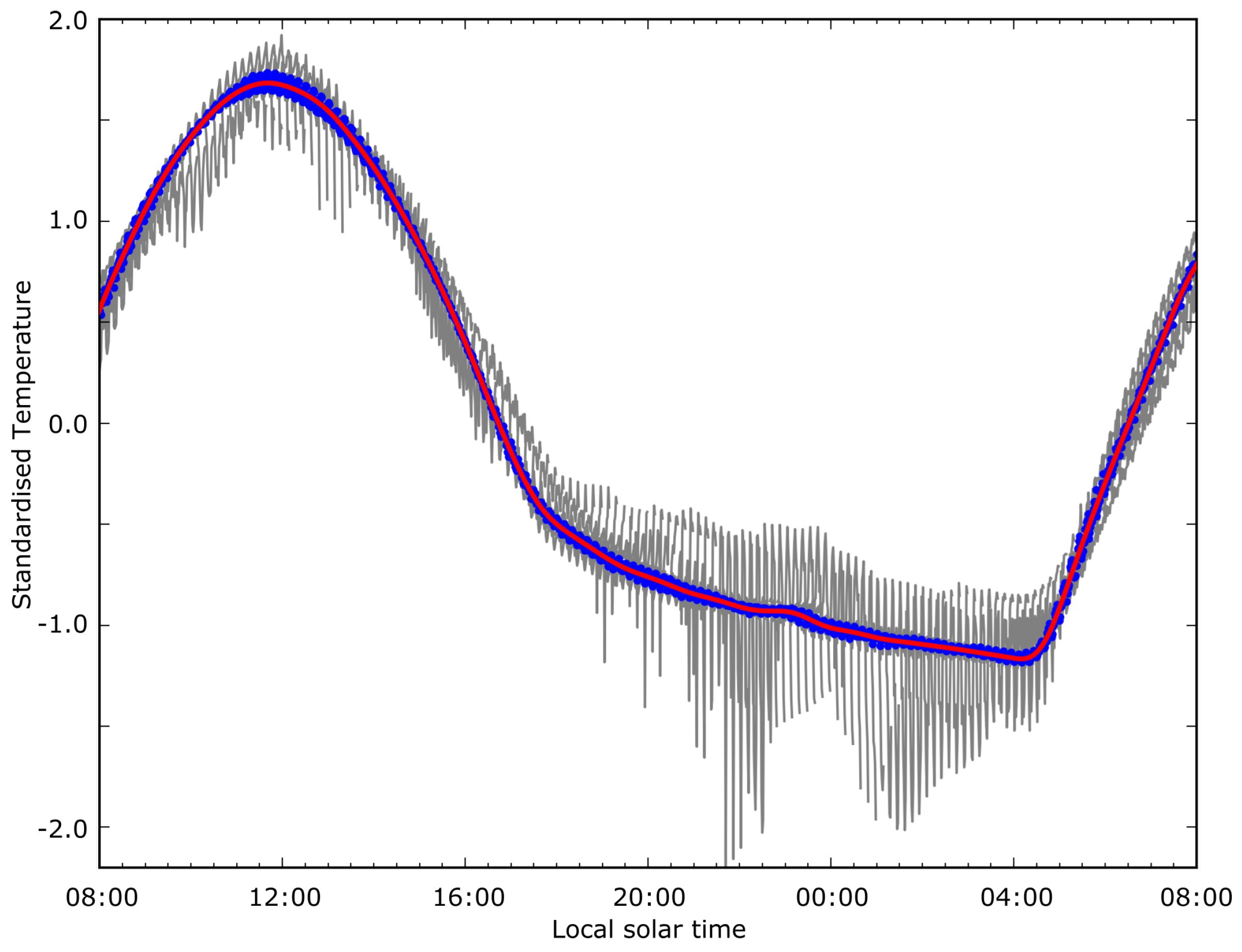
Whilst the accuracy of the fitting method used in this study for days of limited thermal anomalies is quite good, the accuracy of fitting provided by the SVD process breaks down once a large number of anomalies are encountered in the fitted data. This behaviour, which manifests in the type of “wandering” curves displayed in Figure 4c, is caused in part by the standardisation process applied to pixel brightness temperatures, where significant numbers of cloud incidences, especially from thick cold clouds, can act to drop the mean and increase the standard deviation of temperatures across the fitted period. This affects the initial estimation given from the SVD process to the point where the outlier elimination process disregards correct temperature measurements by mistake. One of the limitations of using the SVD fitting method is that outlying measurements in the raw brightness temperatures cannot be easily eliminated from the function evaluation. Whilst applying a more rigorous cloud mask or deriving a standard model for brightness temperatures at a given location and date could be ways of eliminating this mainly low temperature biasing; investigation of other methods for applying the training data for temperature fitting should be a priority.
Overall, the BAT method described in this paper performed adequately from an accuracy standpoint, but the real benefits of the method lie in the improvements in processing time and availability. The BAT method processed an individual fitting at about ten times the speed of the pixel-based training data method, mostly due to the lack of need for cloud mask evaluation of the training data vectors prior to fitting. This issue with the pixel-based training method could be alleviated somewhat by smaller file sizes, as the major issue with processing of the pixel training seems to be the bulkiness of cloud data produced for this sensor (typical file sizes for the AHI cloud product are approximately 90–100 MB). Given the ten day BAT method performed similarly to the pixel-based training method for temperature accuracy, using this data set instead of the thirty day block training set could be justified in situations where processing time of large image sets is of greater importance than extreme accuracy, especially when used for initial anomaly detection purposes.
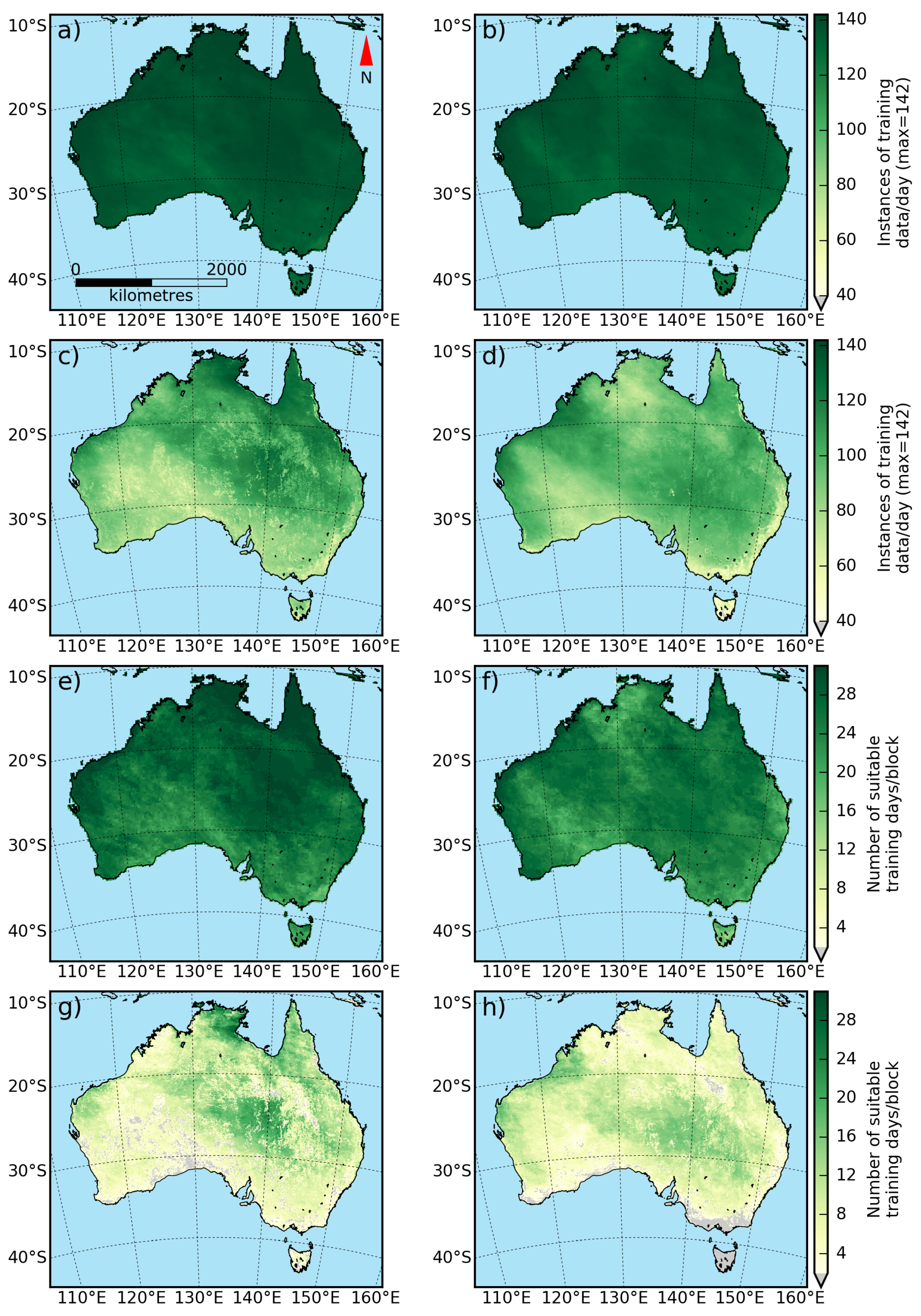
From a fitting availability standpoint, the BAT method significantly increases the distribution of areas that are able to have a temperature fitting applied to them. In comparison to pixel-based methods, the increase of fitting availability is especially marked in areas such as the east and south east coasts and the island of Tasmania. These areas are heavily populated in comparison to much of the Australian continent, and are at significant risk from rapidly changing events, such as fire and flood. The extended utility and application of the BAT method will be of great interest to land management authorities in these areas.
The BAT method formulated in this paper is designed specifically for the process of providing data to inform fitting processes for positive thermal anomaly detection, such as for fire detection. An enhanced understanding of background temperature behaviour in the MWIR space could lead to improvements in the determination of fire detection thresholds, potentially leading to delineation of fire thresholds using time of day, latitude and solar aspect, along with a greater understanding of how the mix of solar reflection and thermal emission in a pixel contributes to the minimum detectable characteristics of a fire from a particular sensor. Applications of this technique could also look to provide ongoing monitoring of fires using metrics such as area, temperature and fire radiative power utilising the improved estimation of this background temperature.
In addition to improvements in the fire detection space, this method could have applications in a number of other fields that require change detection over a short period of time. Likely applications could see aggregation of data based upon land cover classification along with local solar time and latitude to provide a baseline for mapping soil dryness changes, or for tracking the spread and severity of phenomena such as flooding and volcanic activity from geostationary imagery.

5. Conclusions

This study demonstrates the formulation of a broad-area training data derivation method for temperature fitting, for estimation of the background temperature of a pixel measured by a geostationary sensor whilst obscured by cloud, smoke or fire. In comparison to pixel-based methods of deriving training data for temperature fitting, the BAT improves fitting resilience during periods of light to medium obscuration, with fitting errors reduced by more than 50% on days with between 31 and 70 obscured instances using thirty days of training data. The BAT method also demonstrates significant improvement in processing times compared to pixel-based training methods, especially when dealing with a large number of fittings over similar timeframes. The use of the BAT method also increases the availability of training data for fitting purposes, with fitting availability increasing to between 80% and 90% for the time period covered by this study, compared to approximately 40% availability from pixel-based methods. This improved availability of training data will assist in tasks related to the accurate understanding of background upwelling radiation, such as in fire detection and monitoring.

Acknowledgments

The support of the Commonwealth of Australia through the Bushfire and Natural Hazards Cooperative Research Centre is acknowledged. The authors would also like to acknowledge the support of the Australian Bureau of Meteorology, Geoscience Australia, and the Japanese Meteorological Agency for use of AHI imagery associated with this research, along with the Australian National Computational Infrastructure for their support with data access and services.

Author Contributions

B.H., L.W., K.R. and S.J. conceived and designed the experiments; B.H. and L.W. performed the experiments; B.H. and L.W. analyzed the data & B.H., K.R and S.J. wrote the paper.

Conflicts of Interest

The authors declare no conflict of interest. The founding sponsors had no role in the design of the study; in the collection, analyses, or interpretation of data; in the writing of the manuscript, and in the decision to publish the results.

Abbreviations

The following abbreviations are used in this manuscript:
AHI
Advanced Himawai Imager
NOAA
National Oceanic and Atmospheric Administration
ABOM
Australian Bureau of Meteorology
ABI
Advanced Baseline Imager
DTC
Diurnal temperature cycle
SVD
Single value decomposition
LEO
low earth orbit
LST
land surface temperature
CSP
clear sky probability
BAT
broad area training

References

  1. Bowman, D.M.J.S.; Balch, J.K.; Artaxo, P.; Bond, W.J.; Carlson, J.M.; Cochrane, M.A.; D’Antonio, C.M.; Defries, R.S.; Doyle, J.C.; Harrison, S.P.; et al. Fire in the Earth system. Science 2009, 324, 481–484. [Google Scholar] [CrossRef] [PubMed]
  2. Roy, D.P.; Boschetti, L.; Smith, A.M. Satellite remote sensing of fires. In Fire Phenomena and the Earth System: An Interdisciplinary Guide to Fire Science; John Wiley & Sons: Chichester, UK, 2013; pp. 77–93. [Google Scholar]
  3. Calle, A.; Casanova, J.L. Forest fires and remote sensing. In Integration of Information for Environmental Security; Coskun, H.G., Cigizoglu, H.K., Maktav, M.D., Eds.; Springer Netherlands: Dordrecht, The Netherlands, 2008; pp. 247–290. [Google Scholar]
  4. Dozier, J. A method for satellite identification of surface temperature fields of subpixel resolution. Remote Sens. Environ. 1981, 11, 221–229. [Google Scholar] [CrossRef]
  5. He, L.; Li, Z. Enhancement of a fire detection algorithm by eliminating solar reflection in the mid-IR band: application to AVHRR data. Int. J. Remote Sens. 2012, 33, 7047–7059. [Google Scholar] [CrossRef]
  6. Giglio, L.; Kendall, J.D. Application of the Dozier retrieval to wildfire characterization a sensitivity analysis. Remote Sens. Environ. 2001, 77, 34–49. [Google Scholar] [CrossRef]
  7. Giglio, L.; Schroeder, W. A global feasibility assessment of the bi-spectral fire temperature and area retrieval using MODIS data. Remote Sens. Environ. 2014, 152, 166–173. [Google Scholar] [CrossRef]
  8. Giglio, L.; Descloitres, J.; Justice, C.O.; Kaufman, Y.J. An enhanced contextual fire detection algorithm for MODIS. Remote Sens. Environ. 2003, 87, 273–282. [Google Scholar] [CrossRef]
  9. Göttsche, F.M.; Olesen, F.S. Modelling of diurnal cycles of brightness temperature extracted from METEOSAT data. Remote Sens. Environ. 2001, 76, 337–348. [Google Scholar] [CrossRef]
  10. Van den Bergh, F.; Frost, P.E. A multi temporal approach to fire detection using MSG data. In Proceedings of the Third International Workshop on the Analysis of Multi-Temporal Remote Sensing Images 2005, Biloxi, MS, USA, 16–18 May 2005; pp. 156–160.
  11. Roberts, G.; Wooster, M.J. Development of a multi-temporal Kalman filter approach to geostationary active fire detection & fire radiative power (FRP) estimation. Remote Sens. Environ. 2014, 152, 392–412. [Google Scholar]
  12. Hally, B.; Wallace, L.; Reinke, K.; Jones, S. Assessment of the utility of the advanced Himawari imager to detect active fire over Australia. ISPRS Int. Arch. Photogramm. Remote Sens. Spat. Inf. Sci. 2016, XLI-B8, 65–71. [Google Scholar] [CrossRef]
  13. Wickramasinghe, C.; Jones, S.; Reinke, K.; Wallace, L. Development of a multi-spatial resolution approach to the surveillance of active fire lines using Himawari-8. Remote Sens. 2016, 8, 932. [Google Scholar] [CrossRef]
  14. Japan Meteorological Agency. Himawari Standard Data User’s Guide; Technical Report; Japan Meteorological Agency: Tokyo, Japan, 2015. [Google Scholar]
  15. Heidinger, A.K. CLAVR-X Cloud Mask Algorithm Theoretical Basis Document (ATBD); Technical Report; NOAA/NESDIS: Madison, WI, USA, 2004. [Google Scholar]
  16. Majewski, L.; ABOM, Melbourne, Vic, Australia. Personal communication. 2016.
  17. Black, M.; Jepson, A. Eigentracking: Robust matching and tracking of articulated objects using a view-based representation. Int. J. Comput. Vis. 1998, 26, 63–84. [Google Scholar] [CrossRef]
  18. Rajaraman, A.; Ullman, J.D. Mining of Massive Datasets, 2nd ed.; Cambridge University Press: Cambridge, UK, 2011; p. 327. [Google Scholar]
  19. Justice, C.O.; Giglio, L.; Korontzi, S.; Owens, J.; Morisette, J.T.; Roy, D.P.; Descloitres, J.; Alleaume, S.; Petitcolin, F.; Kaufman, Y.J. The MODIS fire products. Remote Sens. Environ. 2002, 83, 244–262. [Google Scholar] [CrossRef]
Figure 1. Time series diagram for a swath of latitude 25.75°S–26°S from 135°E–150°E longitude on 2015 day 319 (15 November 2015). Each square represents the median temperature of the 0.25° block at the image time on the y-axis. These blocks represent one minute of training data that can be fed into the brightness temperature aggregation process.
Remotesensing 09 00167 g001
Figure 2. Figure 1 visualised relative to local solar time. Each of the swaths of block values extracted from each image are shown as a grey line. The four coloured lines depict the trajectory of individual block temperatures at 135°E, 140°E, 145°E and 150°E as the day passes.
Remotesensing 09 00167 g002
Figure 3. An example of the training data fitting process on a swath for a 24-h period. Grey lines represent the raw median values for each swath from the time of each image, the blue data points are representative of the median brightness temperature of the training data at each local solar time, and the red trend line represents the filtered medians of the training data. (Due to the nature of the filtering process, the lack of data at each end of the data results in anomalous fitting and as such the swath sampling has been extended one hour either side of the 24-h period to minimise these errors.)
Remotesensing 09 00167 g003
Figure 4. Examples of model fitting using the four training data derivations. (a) shows a typical day with less than ten cloud instances, (b) shows a day with between 20–30 instances of cloud, and (c) is typical of a day with more than 70 identified cloud periods.
Remotesensing 09 00167 g004
Figure 5. Availability of training data from the block and pixel based methods. (a,b) show the mean instances of training data available using the BAT method for October and November respectively; (c,d) show the training data available using the pixel method for the same months. (e,f) demonstrate the number of 24-h periods that could be utilised as training data for each block in October and November, and (g,h) show this same criteria using the pixel based method.
Remotesensing 09 00167 g005
Table 1. Comparison of MTSAT-2 and AHI-8 sensors for fire detection using a MWIR ( 4   μ m) channel.
SensorMTSAT-2AHI-8
Temporal Resolution30 min10 min
Spatial Resolution (nadir)4 × 4 km2 × 2 km
Medium wave infra-red channel saturation temperature330 K400 K
Quantisation (MWIR)10 bit14 bit
Noise equivalent delta temperature ( N E Δ T )0.09 @ 300 K≤0.16 @ 300 K
Table 2. Comparison of fitting techniques to brightness temperatures recorded by the AHI sensor using root mean square error after eliminating incidences of Clear Sky Probability (CSP) of less than one from the evaluation.
Fitting TechniqueRMS Error (K)
Incidences of CSP < 1≤10 11 30 31 50 51 70 >70
Pixel-based training0.781.012.283.2510.40
BAT (30 days)0.940.941.111.484.19
BAT (10 days)1.151.211.402.106.31
Contextual temperature0.330.420.410.400.42
Number of samples9037417688512345
Table 3. Comparison of time taken to provide a temperature fitting using the pixel-based training technique and the BAT fitting process.
Fitting Technique Time Taken (secs)
BATPre-processing15 mins/day
BAT (30 days)18.4
BAT (10 days)7.3
Pixel-basedSampling cloud statistics141.8
Training & fitting35.5
Total time177.2

