Performance of Smoothing Methods for Reconstructing NDVI Time-Series and Estimating Vegetation Phenology from MODIS Data


1
Department of Physical Geography and Ecosystem Science, Lund University, Sölvegatan 12, SE-223 62 Lund, Sweden
2
Department of Materials Science and Applied Mathematics, Malmö University, SE-205 06 Malmö, Sweden
*
Author to whom correspondence should be addressed.
Remote Sens. 2017, 9(12), 1271; https://doi.org/10.3390/rs9121271
Submission received: 8 September 2017
/
Revised: 1 December 2017
/
Accepted: 4 December 2017
/
Published: 7 December 2017
(This article belongs to the Special Issue Land Surface Phenology )
Abstract
:Many time-series smoothing methods can be used for reducing noise and extracting plant phenological parameters from remotely-sensed data, but there is still no conclusive evidence in favor of one method over others. Here we use moderate-resolution imaging spectroradiometer (MODIS) derived normalized difference vegetation index (NDVI) to investigate five smoothing methods: Savitzky-Golay fitting (SG), locally weighted regression scatterplot smoothing (LO), spline smoothing (SP), asymmetric Gaussian function fitting (AG), and double logistic function fitting (DL). We use ground tower measured NDVI (10 sites) and gross primary productivity (GPP, 4 sites) to evaluate the smoothed satellite-derived NDVI time-series, and elevation data to evaluate phenology parameters derived from smoothed NDVI. The results indicate that all smoothing methods can reduce noise and improve signal quality, but that no single method always performs better than others. Overall, the local filtering methods (SG and LO) can generate very accurate results if smoothing parameters are optimally calibrated. If local calibration cannot be performed, cross validation is a way to automatically determine the smoothing parameter. However, this method may in some cases generate poor fits, and when calibration is not possible the function fitting methods (AG and DL) provide the most robust description of the seasonal dynamics.
1. Introduction
Accurate time-series of vegetation indices from satellite remote sensing are vital for long term vegetation monitoring, especially for studies of vegetation phenology [1] and carbon balance [2,3]. However, the signals received by the satellite sensors are affected by noise due to geometric misregistration, anisotropic reflectance effects, electronic errors, artifacts due to data resampling, atmosphere, and clouds [4]. In order to reconstruct the vegetation seasonal growth course from noisy satellite signals a multitude of time-series processing methods have been used. Some early methods are e.g., the best index slope extraction [5], the repeated moving-window median filter [6,7,8], harmonic functions [9] and median filters [10]. More recently and widely used methods are e.g., Savitzky-Golay filtering [11], least-squares fits to asymmetric Gaussian functions [12] and double logistic functions [13,14,15,16], and variations of spline smoothing [17,18] including the Whittaker smoother [19], and wavelet transforms [20,21,22]. The processing methods can be divided into two broad categories: (1) methods that enable precise capturing of short-term variations during the growing season, generally by employing different types of statistical filters [5,6,10]; and (2), methods that fit mathematical functions (sinusoidal, logistic, Gaussian etc. [12,13,14,15,16,20,21,22]) to part of a season, the full season, or even a sequence of seasons. We can in a loose sense label these as “local” and “global”, respectively, denoting their flexibility to match to details in the time-series or to generalize across the full growing season. Spline methods [17,18,19] have the ability to take on both local and global character depending on a smoothing parameter.
Due to the difficulty of existing physiological process-based phenology models, e.g., various budburst models using chilling or forcing temperature requirements, in accurately simulating phenology from climate data [23], time-series of smoothed vegetation indices measured by satellite are an important data resource for estimating phenology [24,25]. Many studies have employed remote sensing time-series to extract and monitor the timing of plant phenological events [13,15,26,27,28,29]. Since these studies have used different smoothing methods to estimate phenology, it is hard to draw any firm conclusions about which methods are the most suitable. White, et al. [30] compared 10 different phenology retrieval methods applied to an Advanced Very High Resolution Radiometer (AVHRR) NDVI dataset in North America and concluded that although smoothing methods applied to satellite NDVI could generally capture vegetation phenology, no method was universally better than the others. Atkinson, et al. [31] and Chen, et al. [32] concluded that the performance of smoothing methods in estimating vegetation phenology varies spatially and temporally, and that, because of bias and random errors due to cloud influence, no single method exhibited a consistently superior performance. Cong, et al. [33] argued that the reason for not finding a single best method could be different definitions of phenology parameters. Kandasamy and Fernandes [34] highlighted that the performance of different smoothing methods depends on both land surface condition and the clear sky identification approach adopted.
Many studies have investigated the performance of smoothing methods in reconstructing consecutive time-series of vegetation indices, leaf area index and fractional absorbed photosynthetically active radiation (fAPAR) [31,35,36,37,38,39]. Besides vegetation growth time-series from satellite remote sensing, ground-based optical measurements, e.g., Phenocam [40] and multispectral sensors [41,42], have been successfully applied in vegetation phenology studies for different biomes [29] and for linking to satellite remote sensing measurements [43,44]. Also scene-based methods, including geostatistical methods, have been used to investigate the effects of time-series smoothing [19]. However, despite the multitude of studies there is a lack of agreement regarding the choice of time-series smoothing methods.
To investigate the usefulness of time-series smoothing methods it is appropriate to test the ability of the methods to reconstruct the seasonal variation of the temporal signal. This can best be done by directly relating it to ground measurements. Today, growing networks of ground measured reflectance measurements exist, suitable for process studies and validation of remotely sensed vegetation index data [45,46].
Furthermore, some indirect data may provide useful time-series records for establishing the ability of different time-series methods to portray the vegetation dynamics. One of these is gross primary productivity (GPP) estimated from carbon flux measurements. This is based on the assumption that GPP is related to the satellite derived NDVI. The relationship between NDVI and fAPAR has been investigated by Asrar, et al. [47] and Sellers, et al. [48], and it has been used as major input in models to estimate GPP [2,3,49]. This relationship implies that GPP is a useful reference for evaluating the abilities of different methods for smoothing satellite NDVI.
Also spatial data may be useful for investigating the different methods. It is well known that topography influences vegetation phenology due to adiabatic temperature difference with height. At high elevation of temperate and boreal regions, slow thermal accumulation leads to delayed canopy development [50,51] and generally shorter growing seasons than those at low elevation. Based on this concept, a number of studies have used elevation gradients to spatially investigate phenology from satellite data e.g., [15,52,53].
Given the difficulty in drawing firm conclusions about different smoothing methods from previous studies, this study aims to address the following questions: (1) is it possible to define one smoothing method that is always best suited, irrespective of situation; (2) if not, what capability do the different methods have for smoothing data in different situations. To achieve this aim, we evaluate the performance of smoothing algorithms for representing seasonal vegetation growth with 8-day MODIS NDVI data by employing a variety of reference data sets. We systematically analyze five different smoothing methods: Savitzky-Golay filtering (SG), locally weighted regression scatterplot smoothing (LO), spline smoothing (SP), least-squares fitting to asymmetric Gaussian functions (AG), and least-squares fitting to double logistic functions (DL), against three different reference data sets: ground measured NDVI from ten locations, ground measured GPP from four sites, and elevation data from an uphill area with a vegetation gradient. Altogether these analyses will support our aim and allow better understanding of how to choose suitable time-series smoothing methods for remote sensing phenology studies.
2. Materials and Methods
2.1. MODIS NDVI Data and Ground Reference Data
The MODIS/Terra MOD09Q1 land surface reflectance dataset of 8-day interval and 250 m spatial resolution [54] was used as an example in this study. We used the binary MODIS quality flags to set weights for each observation. NDVI time-series from 2000 to 2014 were calculated using near-infrared (NIR) and red reflectance from MOD09Q1 for the 10 field sites and the test area with elevation reference data. For each field site, the reflectance data of single pixels were used rather than the mean value of several neighboring pixels, so that the performance of smoothing methods on single pixel time-series data could be fully evaluated.
For ground reference, NDVI data from sensors mounted on masts at 10 sites (Figure S1 in Supplementary Material), located in Scandinavia, Greenland and Africa, were used [42,55]. These sites cover different environments: arctic, sub-arctic, deciduous forest, evergreen forest, grassland, savanna, and clear-cut forest (Table 1) and the sites were established in homogeneous areas in terms of vegetation coverage and topography. The sensor pairs were calibrated following Jin and Eklundh [56]. Ground-based NDVI was computed from daily noontime reflectance in red and NIR bands, and it agreed very well with MODIS data during the growing season [42]. For further information about the field measurements, see Eklundh, et al. [42]. To agree with the time step of MOD09Q1 NDVI, daily NDVI were converted to 8-day NDVI values by median filtering. Due to the high latitude of sites 1–7, snow cover in winter disturbed both spectral NDVI sensors on the ground and MODIS. For this reason, we only compared them during the non-winter period: April–October at the Hyytiälä and Norunda sites and June–September at the Abisko and Zackenberg sites [57,58,59,60].
We used flux-tower measured GPP from sites Fäjemyr, Zackenberg, Hyytiälä and Norunda Forest (Table 1) to evaluate the performance of the time-series smoothing methods for estimating vegetation temporal dynamics from the satellite images. Weekly (8-day) GPP data for these sites were acquired from Fluxnet (http://www.eosdis.ornl.gov/FLUXNET).
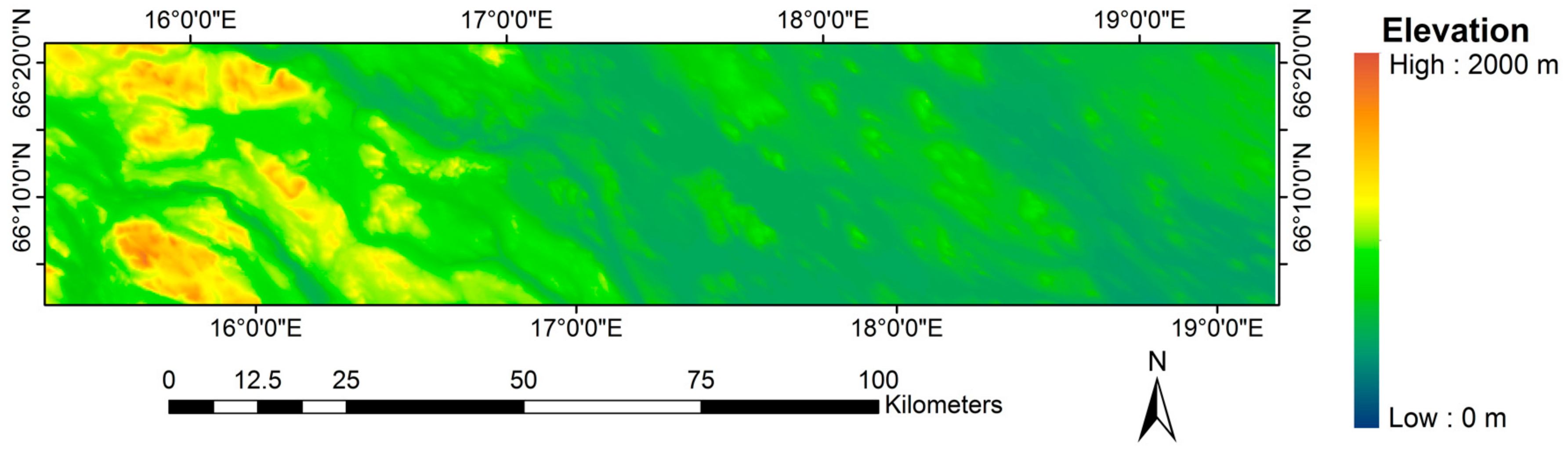
Besides using ground reference data from point locations, we used spatial data from the Ammar region, located in Västerbotten, Sweden, and having a significant elevation gradient (approximately 1980 m). Elevation data (50 m spatial resolution) were obtained from the Swedish mapping, cadastral and land registration authority, Lantmäteriet (Figure 1). It was resampled to 250 m and matched to MOD09Q1 pixels. The reason for selecting the Ammar region is that the Ammar region represents a gradient of changing elevation from low to high, and vegetation varying from dense to sparse with elevation. In addition, the region has stable land cover (mainly forest and natural vegetation classes) with few logging activities or pest disturbances reported during the studied period.
2.2. Time-Series Smoothing Methods
Since it is beyond our capacity to investigate all possible time-series smoothing methods we have selected some common methods from the two broad categories of local vs global methods. From the local category we have chosen adaptive Savitzky-Golay filtering (SG) [11,61] and adaptive LOESS filtering (LO) [62], and from the global category we have chosen least-squares fits to asymmetric Gaussian functions (AG) [12] and double logistic functions (DL) [13,14]. In addition, we test spline smoothing (SP) [63,64] that has capacity to act both as a local and a global smoother.
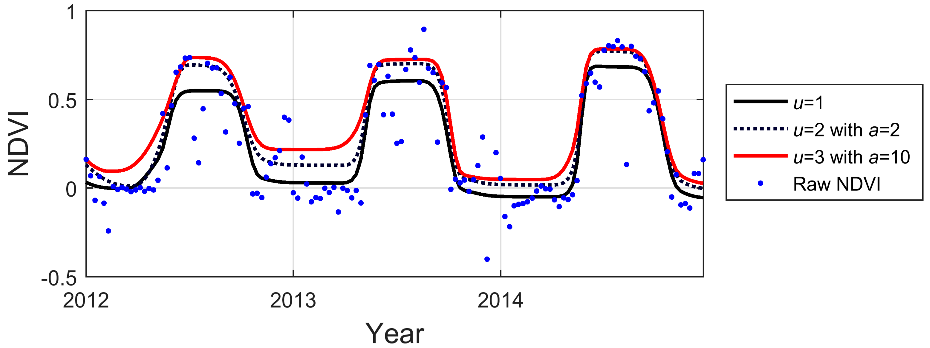
SG, AG and DL are available in the current TIMESAT version 3.3 [16,65]. LO and SP were integrated into a development version of TIMESAT for this study. The adaption to the upper envelope of the original NDVI time-series was applied to all smoothing methods for reducing negative bias of satellite NDVI due to clouds or poor atmospheric conditions [11,16]. Upper-envelope adaptation makes the smoothed function approach the upper NDVI envelope by iteratively generating new curves with data weights that have lower values for the data points below the previous smoothed curve [11,12]. This upper-envelope adaptation is in TIMESAT determined by two parameters: the number of iterations for which weights are being modified, and the adaptation strength , which fine-tunes the strength of the upper-envelope weighting in each iteration (Figure 2).
2.2.1. Polynomial Local Filtering (SG and LO)
The principles of SG and LO are similar in that both methods replace each data value by a combination of adjacent values in a window using a least-squares second-order polynomial fit (Figure 3 and Figure 4). The size of the filtering window determines the degree of smoothing. If rapid variations are encountered in the window, both methods are in TIMESAT modified to automatically decrease the window size. This enables quite sudden variations in the NDVI trajectory to be modelled. In this study, the definition of the filtering window size r in both smoothing methods is the same as in TIMESAT, i.e., , where is the number of time steps from right/left to the middle point m.
The difference between SG and LO is in the weights of each data point in the filtering window. In SG, all points of the fitting window have weight 1.0, whereas in LO weight of point decreases outwards from the middle point m of the filtering window
If the same window size is applied to both methods, the different weighting systems cause LO to have lower total data weight than SG. In other words, LO has to have a larger window size than SG to result in the same data smoothing effect as SG. A benefit of LO is that it prevents some of the sharp peaks often encountered in SG filtering.
In this study, we tested varying in SG from 2 to 7, and equivalently varying in LO from 4 to 12 (Table 2).
2.2.2. Spline Smoothing (SP)
We adapted the Fortran code by Woltring [64] to achieve spline smoothing based on the description in Craven and Wahba [63]. The Whittaker smoother [66,67] can be considered as a special case of spline smoother [68]. Spline smoothing is employed to find a spline function that minimizes the value of a criterion function for a selected smoothing parameter ,
where is a regularly spaced time grid and the corresponding NDVI values. Each point in the time-series is associated with a weight . is a vector containing an adaptive stiffness weight for each . The smoothing parameter controls the shape of the spline, varying from an exactly interpolating spline () to a straight line () (Figure 5).
Instead of manually selecting suitable , an alternative automatic approach is to use generalized Cross-Validation (CV), which was described by Craven and Wahba [63] and implemented in the Fortran code based on the improvement by Woltring [64]. In this study, we tested SP with CV (SPCV) and without CV, respectively. We also implemented CV in our code for the SG and LO methods to automatically choose the parameter and to be able to compare the effect of CV on these methods with the effect on SP. The range of in SP was limited to produce local fits, which means that we forced the performance of SP to be fairly close to SG or LO. In this case was set to the range 0.1–10 with exponential intervals, i.e., 0.1, 0.25, 0.63, 1.58, 3.98 and 10 (Table 2).
Differently from the upper-envelope iterations in the other smoothing methods, the upper-envelope iterations in SP and SPCV also updates each based on the formula:
where is the amplitude of all , and is the amplitude of in the window from to , in which was set to 5, i.e., a quarter of one year’s data; is the stiffness adaptation strength, which is in the range from 0 to close to 1, where 0 will give no local adaptation and close to 1 will give very high local adaptation. The adaptation factor was integrated into SP to locally adjust the curve shape. In the original code spline stiffness is governed by . A large value of gives a stiff spline, and a low value of gives a spline that is flexible. However, a large value of may result in low absolute values of the derivative in the spring and the autumn, resulting in poor fits during these seasons. The idea with the adaptive method is to give each point a stiffness by multiplying the global stiffness parameter with an adaptation factor . The adaptation factor should be such that it is close to 1 for points in the summer/winter and smaller, i.e., 0.1, at points in the spring/autumn, where the season changes rapidly (Figure 6), see also Lamm [69]. In this study, was tested at values 0.1, 0.3, 0.5, 0.7 and 0.9 (Table 2). While iterating to adapt to the upper-envelope in SPCV, the values calculated from the first iteration were locked and applied in the remaining iterations.
2.2.3. Least-Squares Fits to Model Functions (AG and DL)
2.3. Performance Assessment of the Time-Series Smoothing Methods
2.3.1. Ground Measured NDVI Time-Series vs. Smoothed Satellite NDVI
The root mean squared error (RMSE) between smoothed satellite NDVI time-series and ground-based NDVI time-series was used to evaluate the accuracy of each smoothing method. In most cases, the method generating the minimum RMSE can be considered the most accurate, and it thereby indicates the optimal capability of the method. However, for unknown areas where ground reference data are lacking, which is commonly the case in operational remote sensing applications, the optimal parameter settings for each method is unknown. Therefore, we also computed the median RMSE and the range of RMSE from all possible settings for a single method. Together, the minimum, median and range provide a general description of the performance of each method. The minimum indicates the best performance of each method given that calibration data are available. When no calibration data are available, the median and range are better indicators, providing information on the average performance and the associate range of each method. A large range indicates a flexible method, meaning that both low and high accuracy could be attained.
2.3.2. Ground Measured GPP Time-Series vs. Smoothed Satellite NDVI Time-Series
We employed Spearman’s rank correlation coefficient () to measure the synchronized variation (not necessarily linear) between ground measured GPP and smoothed NDVI time-series. When GPP and NDVI are unsynchronized, the Spearman correlation is 0, and when they co-vary monotonically it is ±1.0. We used non-winter period GPP data for comparison only during the vegetative season.
2.3.3. Elevation vs. Phenology Parameters from Satellite NDVI Data
Besides evaluating the performance of the smoothing methods for reconstructing time-series, we evaluated their abilities for extracting phenological metrics across a spatial gradient. The assumption of the experiment was that in this area the variation of vegetation phenology, such as start of the season (SOS), end of the season (EOS), length of the season (LOS) and small seasonal integral (SI) along the gradient, are generally related to average air temperature [23,51], and that this is partly controlled by the local elevation. Other factors, such as solar radiation, hydrology, soil type, etc., also affect the relationship [23], but we assume that for comparing the different smoothing methods the influence of these is negligible. We extracted SOS, EOS, LOS and SI by TIMESAT based on smoothed MODIS NDVI time-series. To avoid inter-annual variations we averaged the phenology variables over the 10 years between 2001 and 2010, which reduces influences of trends and extreme events, and emphasizes phenological variation along the elevation gradient. To avoid effects of non-linearity we used Spearman’s rank correlation coefficient for detecting the relationships. For extracting phenological metrics from time-series, suitable thresholds to define start and end of season are required. Since NDVI has a strong response to snow [70] and MOD09Q1 does not have snow flags, using high amplitude thresholds is necessary to avoid capturing snow dynamics rather than dynamics of vegetation. Therefore, the thresholds for start and end of season were set to a high value of 72% of the amplitude, which was based on Fennoscandian studies by [71,72]. For the same reason we did not use derivatives for determining SOS and EOS, which would have been strongly influenced by snow seasonality during early and late parts of the seasons.
3. Results
3.1. Ground Measured NDVI Time-Series vs. Smoothed Satellite NDVI Time-Series
RMSE values for the 987 runs with different settings for the smoothing of MODIS NDVI are displayed as averages (Table 3) and as boxplots for each of the sites and methods (Figure S2). Overall, for the ten test sites, average RMSE of the raw MODIS NDVI and ground-measured NDVI was 0.14 (Table 3). After applying smoothing, RMSE was on average reduced to 0.08, and the range of RMSE was 0.06. Most sites (89% of the 987 simulations) showed reduced RMSE compared to raw data, except at Sudan Barah. At the sites with high NDVI values and long growing season, such as Abisko Delta, Abisko Stordalen, Fäjemyr, Hyytiäla and Norunda forest, the reductions in RMSE were larger than at the other sites that have lower NDVI or shorter growing seasons. The difference can be partly attributed to cloud effects. Clouds contribute to the majority of noise in the satellite received vegetation signal during the growing season. Hence, sites with high NDVI values are more strongly affected by cloud contamination than sites with low NDVI. In addition, the dry Sudanian sites have short growing season, and there is generally lower cloud contamination than in the humid areas. As a result, smoothing methods have a weaker effect on the RMSE than at the humid sites with high NDVI values and long growing seasons.
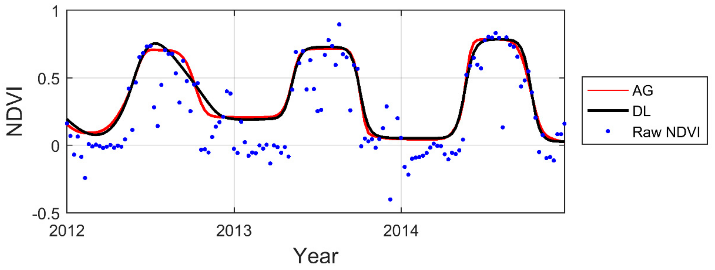
When studying each smoothing method, we found that the minimum and median RMSEs of all methods differed relatively little, but that overall LO generated slightly lower RMSE than the other four methods (Table 3). Although window size q in SG/LO and smoothing parameter p in SP have different definitions, these methods produced similar smoothed time series (Figure S2). DL generated the smallest RMSE range of 0.035. The function fitting methods AG and DL also generated very similar results to one another. SP was closer to the local filtering methods. Cross validation (SGCV, LOCV and SPCV) generated RMSE values lower than median RMSE in most cases (87%), which means that CV is in many cases able to assist in selecting satisfying settings for a single pixel. In four out of the 30 cases, CV resulted in very poor results. When comparing the methods across the ten test sites, SG and LO produced the eight lowest RMSE values out of the ten test sites, except at the Hyytiälä site and the Demokeya site where AG and SP produced the lowest RMSE respectively. The lowest median RMSEs varied between methods at the different sites, without any clear pattern. The smallest RMSE ranges were produced by the function-fitting methods (AG and DL) for nine sites. At one site, Sudan Barah, which had the lowest NDVI and the shortest growing season of all, this was not true. This may be due to the large NDVI uncertainties from measurement when NDVI is small [56]. The time-series patterns generated from each method are shown in Figure S3. SG, LO, SP were able to describe the variation of NDVI during the growing seasons (e.g., year 2011 in Figure 8). However, AG and DL were more robust in reconstructing the general seasonal patterns when MODIS NDVI was noisy (e.g., year 2010 in Figure 8). For details of time-series patterns generated from each method for all 10 sites, see Figure S3.
In conclusion, this experiment showed that applying smoothing methods to MODIS NDVI reduced differences with ground-measured NDVI. The local filtering methods (SG and LO) had better performance in representing ground NDVI from MODIS NDVI with optimized setting parameters, but the function fitting methods (AG and DL) were more robust in the sense that they generated less varying results depending on how the settings were chosen. CV for automatically choosing smoothing parameters generated better-than-average fits for the majority of SG, LO and SP runs, however it failed in a few cases.
3.2. Ground Measured GPP Time-Series vs. Smoothed Satellite NDVI Time-Series
At the four flux measurement sites, of non-smoothed 8-day MODIS NDVI and GPP was 0.338 on average (Table 4). After applying smoothing, on average increased up to 0.513, and the range between the best and the worst case was 0.228 (Table 4). In 98% of the runs, the tested methods successfully increased values at the four test sites (Table S3). The method that produced the highest maximum values varied between the sites.
When comparing the smoothing methods, we note that the highest maximum and median ρ were generated by AG of 0.673 and 0.555, respectively (average for four sites). However, they varied among sites (Table S3). CV automatically selected fairly suitable smoothing parameter for SP but sometimes failed for SG and LO. In contrast to the previous experiment, the local filtering methods did not generate the highest ρ even with the optimized settings. The smallest range of ρ was generated by DL, which was similar to the first experiment.
In conclusion, this experiment showed that applying smoothing methods to MODIS NDVI improved covariation with ground-measured GPP. No single method always generated the best results in representing NDVI time-series highly correlated with GPP time-series, but AG and DL were more robust in the sense of being less influenced by individual settings.
3.3. Elevation vs. Phenology Parameters from Satellite NDVI Data
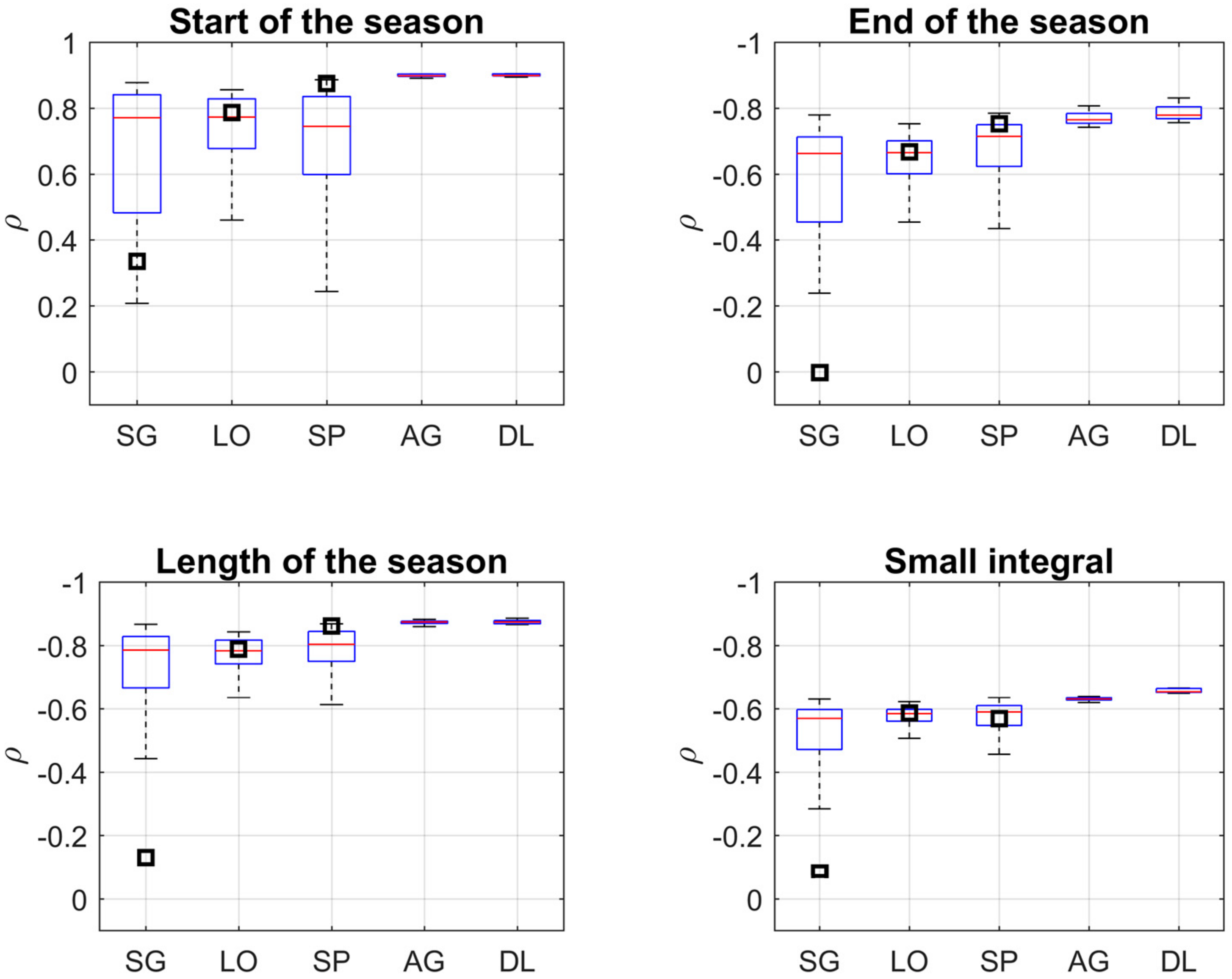
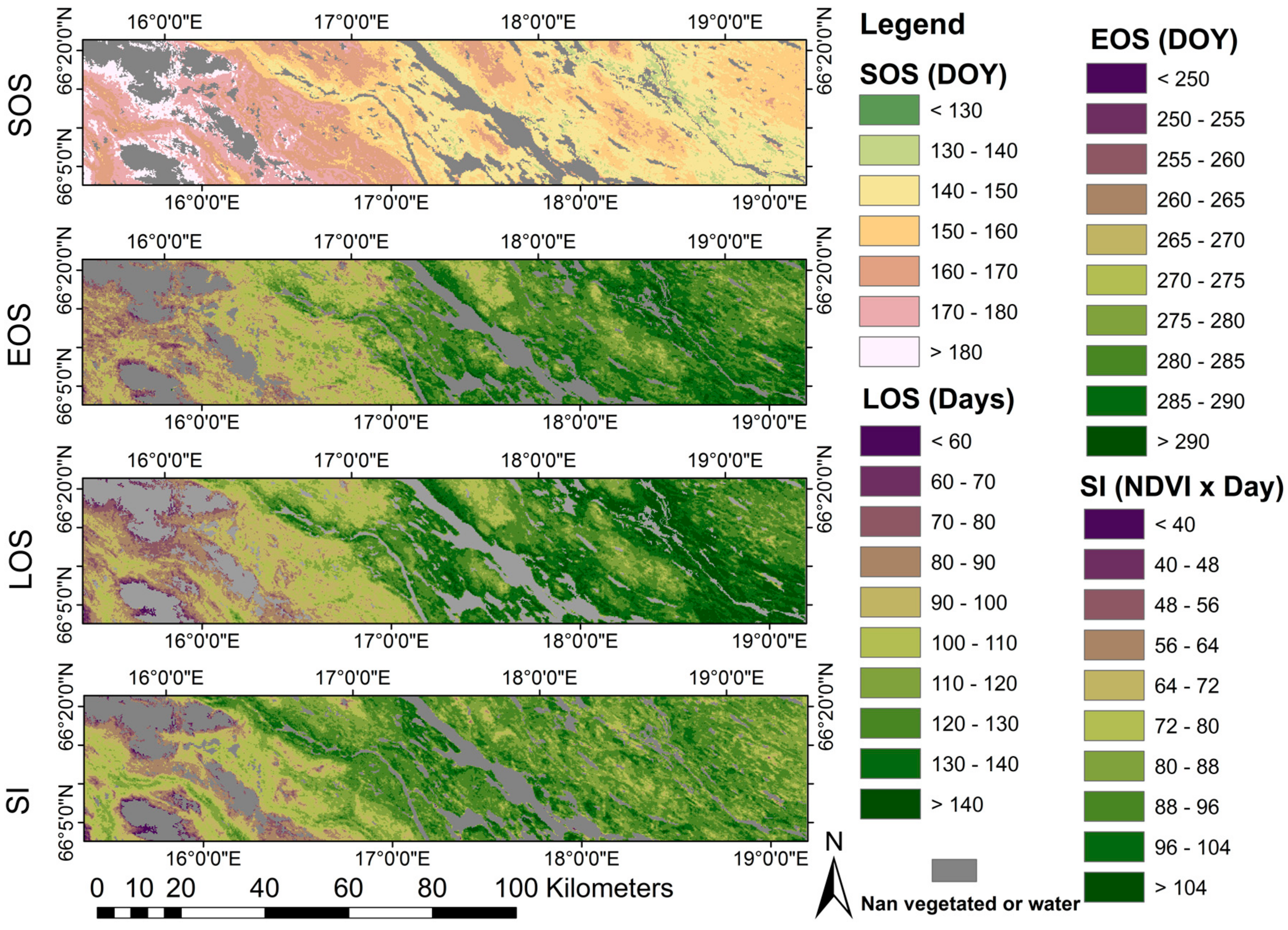
The correspondences between elevation and phenological parameters are shown in Figure 9 and Table 5. Positive ρ values for SOS means that SOS occurs later with increasing elevation, whereas negative ρ values for EOS, LOS and SI means that EOS occurs earlier, LOS is shorter, and SI is smaller with increasing elevation. DL produced the highest absolute maximum and median ρ values (Table 5 and Table S4). The smallest ranges of ρ were generated with AG and DL. The ranges of ρ produced by AG and DL were much smaller than those produced by SG, LO and SP. CV was able to generate similar or higher absolute ρ for LO and SP in most cases, and for SP results from CV were very good. However, for SG it generated much lower absolute ρ. Phenological maps generated with optimized DL settings (Figure 10) show coherent spatial patterns and correspondence with elevation in Figure 2. In general, the experiment showed that the function fitting methods, especially DL, performed better than the other methods for extracting generalized vegetation phenology.
4. Discussion
In this study, we demonstrated the degree to which five smoothing methods (SG, LO, SP, AG and DL) improved MODIS NDVI time-series data for representing ground-measured NDVI, ground measured GPP, and for extracting phenological parameters correlated with topographical elevation. To cover a range of possible settings chosen by users we employed a total of 987 different settings for the five smoothing methods in each experiment. The three independent experiments together provide insights in the choice of methods across different sites.
4.1. Which Smoothing Method is the Most Accurate
The local filtering methods SG and LO have very similar definitions, although LO has a more advanced weighting system than SG. Despite this, the results from LO were not clearly better than those from SG. The explanation may be that LO assigns very high weight to the middle data point in the smoothing window and gives low weights to the other points. This leads to a more pronounced ‘local’ characteristic for LO, which may be negative in the presence of strong noise. On the other hand, this ‘local’ characteristic may be an advantage for detecting detailed changes during a growing season. In many cases the local methods were superior for reconstructing ground NDVI. However, the differences in RMSE were small and may be due to random chance.
Spline smoothing has the advantage of having only one parameter, p, to change the degree of smoothness of a curve. However, the performance of SP was not better than the other methods in any of the three experiments. This could partly be explained by a limited number of tested p values. p can be set to any positive natural number, but in this paper p was only tested for six selected values, which means that the full capability of SP was not utilized. SPCV generated more robust results than SP, but it had poorer performance in generating results in optimized parameters. When applying SPCV to images it optimizes p for every pixel. However, it can be questioned whether is it reasonable to allow different degrees of smoothing for different pixels, irrespective of their class membership. The third experiment showed that SPCV performed better than SG, LO and SP but worse than AG and DL.
Contrary to the other methods, AG and DL smooth data in a static window (half/full seasons), which is the reason for their robustness. In addition, AG and DL tend to eliminate noise at peaks and valleys in a time-series. Although this elimination limits the ability of AG and DL in detecting detailed variations during periods near the season peak, it helps to automatically and robustly extract temporal phenology variables, e.g., SOS, EOS, and LOS (third experiment). The results of our tests point to the superiority of these function fitting methods for extracting phenological parameters over large areas where calibration of the smoothing parameters is not possible.
4.2. How to Choose Smoothing Methods
Since there is no single method that is always optimal, selecting a suitable smoothing method depends on the data quality, signal dynamics, and the intended level of generalization of the smoothing. We found that in general, the function fitting methods are robust for extracting phenological parameters or reconstructing strongly generalized seasonal curves. Function fitting methods are also the prior choice for smoothing data with very low quality (e.g., frequent noise and gaps). However, these methods have a limitation when it comes to capturing curve details and risk of underfitting, thereby compelling us to sometimes use local filtering methods. If the purpose is to analyze intra-seasonal variations (e.g., in disturbance analyses), local filtering methods are recommended, because they are able to capture seasonal details. Also, if there are multiple peaks during the season (e.g., due to multiple harvesting in agricultural lands), local filtering methods may be more useful because their smoothing process is freer. Function fitting methods may work also with multiple cropping but a difficulty is to provide initial positions and shapes for the functions of all seasons.
4.3. How to Choose Smoothing Parameters
The efficiency of each smoothing method depended on the choice of parameters. For example, applying upper-envelope iterations generally improved the results. This emphasizes the need to further compensate time-series of MODIS 8-day composite NDVI data for remaining negative bias due to cloud and aerosols in the atmosphere. At the sites Barah and Demokeya, where upper-envelope iterations did not improve results, vegetation density was very low, which means that the data were probably more affected by soil background characteristics, which would lead to decreased noise bias. When comparing against GPP, upper-envelope iterations also generally improved results, except when using DL and SPCV at the Norunda forest site. In the third experiment, upper-envelope iteration of SPCV, AG and DL did not improve ρ in correlating end of season timing and elevation, which could help explain why upper-envelope iterations also did not improve DL and SPCV fits at the Norunda forest site.
The smoothing parameters, q in SG and LO, and p in SP, were much more influential than the envelope parameters u and a in the first experiment. As a consequence, more attention needs to be paid to adjusting q and p. In addition, the ability to vary the smoothing parameters q and p means that SG, LO, and SP have larger flexibility than AG, and DL, but this flexibility means that the methods are less robust to user selection of parameter values. A higher flexibility means that a method is more capable of matching satellite data with ground reference data, but accurate matching also requires ground observations for calibration. In most situations, this calibration is impossible due to a lack of ground observations, and, as seen from the large ranges observed in the second and third experiments, a robust method with fewer parameters may be preferred.
Automatically selecting smoothing parameters by CV can be useful for SG, LO and SP if no ground reference data are available for calibration, as demonstrated by the above-average results achieved with this technique. However, applying CV can sometimes lead to very poor results, as seen in a few cases (e.g., Abisko and Hyytiälä in Figure S2). CV may also result in different parameter settings being used for different pixels of the same land cover class, and it can be discussed if this is reasonable. It can also be noted that CV had different effects on SP as compared to SG and LO. In SP, the smoothing parameter is continuous, whereas it is discrete in SG and LO. The discrete parameters in SG and LO may lead to unsatisfactory results if the data quality is poor and the smoothing parameter significantly influences the fitting, which could be the reason that CV is less reliable for SG and LO than for SP.
Although most smoothing methods improved the ability of the satellite time-series to represent the ground reference data, it was not possible to find a single parameter setting that was always able to generate suitable results for all environments, which supports the finding by Hird and McDermid [35] and Atkinson, et al. [31].
4.4. Limitations of this Study and Future Possible Directions
Besides NDVI, there are many optional indexes used to describe vegetation time-series dynamic such as the Enhanced Vegetation Index [73] and the plant phenology index [60]. Different indexes could present different time-series patterns for the same pixel, which could lead to different conclusions for different smoothing methods. Moreover, the difference between data from different satellite sensors, such as MODIS and NDVI3g, could also lead to different estimates of phenological parameters [74]. In addition, although the tested sites represent several different biomes, it cannot be ruled out that other vegetation types with different seasonal profiles might yield differences in relationships with ground reference data. Furthermore, although the sites used in the first and second experiments were generally spatially homogeneous, uncertainties in footprint matching may have affected the relationships. In the last experiment, it is recognized that several factors other than elevation affect the general phenology in the area. It is unknown if and to what degree these different factors affect differences in performance between the different smoothing methods. The results of this study are valid for the tested data and sites, and relationships may change with other data or under different conditions. However, the consistency of the results indicates a general validity of the conclusions also outside the tested domain.
5. Conclusions
In this paper, we utilized three ground reference data sets for evaluating the performance of five smoothing methods in processing MODIS NDVI time-series. We conclude that the smoothing methods reduced the error between MODIS NDVI and ground-measured NDVI in 89% of the simulations, and that they improved the covariation between MODIS NDVI and ground-measured GPP in 98% of the simulations. It is possible to achieve very good similarity with ground NDVI data with the local filtering methods (Savitzky-Golay and LOESS smoothing) when parameters are finely tuned. However, on average the differences between the methods were small and it is not possible to conclusively recommend a single method in favor of the others. Spline smoothing did not generate better results than any of the other methods, but using cross validation generally improved the spline fits and gave fairly good results. Cross validation was also useful for selecting parameters for Savitzky-Golay and LOESS smoothing; however, in some cases the method failed. The function fitting methods (double logistic and asymmetric Gaussian functions) showed the best performance for estimating average phenology across a topographic gradient. The function fitting methods were also found to generally reduce the risk of achieving very poor results (shown by the smaller range of output results), thus they are safer than the other methods to use when it is not possible to carry out any calibration against ground measurements.
Supplementary Materials
The following material is available online at www.mdpi.com/2072-4292/9/12/1271/s1, Figure S1: Geographic distributions of ground-based spectral observation sites and Ammar region, Figure S2: Boxplots of RMSEs between ground-based measured NDVI and smoothed satellite NDVI, Figure S3: Plots of smoothed curves of each method at all testing sites based on the settings that provide the minimum RMSE values, Table S1: Additional information of ground-based spectral observation sites and flux tower sites, Table S2: The minimum, median and range of RMSE between smoothed MODIS NDVI from all settings of each smoothing algorithm and ground measured NDVI from all spectral sensor tower sites, Table S3: Maximum, median and range of ρ between smoothed MODIS NDVI from all settings of each smoothing algorithm and ground measured GPP, Figure S4: Boxplots of Spearman’s rank correlation coefficient of tower GPP and smoothed MODIS NDVI for each method, showing the distribution with different settings at test sites, Table S4: The maximum, median and range of ρ between elevations and land surface phenology parameters extracted by each smoothing algorithm of all settings on MODIS NDVI.
Acknowledgments
The research was funded by a grant from the Swedish National Space Board to Lars Eklundh and Per Jönsson, Dnr. 119/13. We acknowledge access to flux data from ICOS Abisko station, Hyytiälä station, Norunda station Sweden, ICOS Finland, and Fluxnet. We thank Dr. Jonas Ardö for providing spectral data for the Sudan sites. The MOD09Q1 data product was retrieved from the online Data Pool, courtesy of the NASA EOSDIS Land Processes Distributed Active Archive Center (LP DAAC), USGS/Earth Resources Observation and Science (EROS) Center, Sioux Falls, South Dakota, https://lpdaac.usgs.gov/data_access/data_pool.
Author Contributions
Z.C., P.J. and L.E. conceived and designed the experiments; Z.C., H.J. and L.E. performed the experiments; Z.C. and L.E. analyzed the data; P.J. and L.E. contributed analysis tools and field equipment; Z.C. and H.J. wrote the manuscript draft with further contributions by L.E. and P.J.
Conflicts of Interest
The authors declare no conflict of interest. The founding sponsors had no role in the design of the study; in the collection, analyses, or interpretation of data; in the writing of the manuscript, and in the decision to publish the results.
References
- Schwartz, M.D. Phenology: An Integrative Environmental Science; Springer: Dordrecht, The Netherlands, 2003; Volume 346. [Google Scholar]
- Prince, S. A model of regional primary production for use with coarse resolution satellite data. Int. J. Remote Sens. 1991, 12, 1313–1330. [Google Scholar] [CrossRef]
- Running, S.W.; Nemani, R.R.; Heinsch, F.A.; Zhao, M.; Reeves, M.; Hashimoto, H. A continuous satellite-derived measure of global terrestrial primary production. Bioscience 2004, 54, 547–560. [Google Scholar] [CrossRef]
- Goward, S.N.; Markham, B.; Dye, D.G.; Dulaney, W.; Yang, J. Normalized difference vegetation index measurements from the advanced very high resolution radiometer. Remote Sens. Environ. 1991, 35, 257–277. [Google Scholar] [CrossRef]
- Viovy, N.; Arino, O.; Belward, A. The Best Index Slope Extraction (BISE): A method for reducing noise in NDVI time-series. Int. J. Remote Sens. 1992, 13, 1585–1590. [Google Scholar] [CrossRef]
- van Dijk, A.; Callis, S.L.; Sakamoto, C.M.; Decker, W.L. Smoothing vegetation index profiles: An alternative method for reducing radiometric disturbance in NOAA/AVHRR data. Photogramm. Eng. Remote Sens. 1987, 53, 1059–1067. [Google Scholar]
- Menenti, M.; Azzali, S.; Verhoef, W.; van Swol, R. Mapping agroecological zones and time lag in vegetation growth by means of Fourier analysis of time series of NDVI images. Adv. Space Res. 1993, 13, 233–237. [Google Scholar] [CrossRef]
- Olsson, L.; Eklundh, L. Fourier series for analysis of temporal sequences of satellite sensor imagery. Int. J. Remote Sens. 1994, 15, 3735–3741. [Google Scholar] [CrossRef]
- Zhu, Z.; Woodcock, C.E.; Olofsson, P. Continuous monitoring of forest disturbance using all available Landsat imagery. Remote Sens. Environ. 2012, 122, 75–91. [Google Scholar] [CrossRef]
- Reed, B.C.; Brown, J.F.; VanderZee, D.; Loveland, T.R.; Merchant, J.W.; Ohlen, D.O. Measuring phenological variability from satellite imagery. J. Veg. Sci. 1994, 5, 703–714. [Google Scholar] [CrossRef]
- Chen, J.; Jönsson, P.; Tamura, M.; Gu, Z.; Matsushita, B.; Eklundh, L. A simple method for reconstructing a high-quality NDVI time-series data set based on the Savitzky–Golay filter. Remote Sens. Environ. 2004, 91, 332–344. [Google Scholar] [CrossRef]
- Jönsson, P.; Eklundh, L. Seasonality extraction by function fitting to time-series of satellite sensor data. IEEE Trans. Geosci. Remote Sens. 2002, 40, 1824–1832. [Google Scholar] [CrossRef]
- Zhang, X.; Friedl, M.A.; Schaaf, C.B.; Strahler, A.H.; Hodges, J.C.; Gao, F.; Reed, B.C.; Huete, A. Monitoring vegetation phenology using MODIS. Remote Sens. Environ. 2003, 84, 471–475. [Google Scholar] [CrossRef]
- Beck, P.S.; Atzberger, C.; Høgda, K.A.; Johansen, B.; Skidmore, A.K. Improved monitoring of vegetation dynamics at very high latitudes: A new method using MODIS NDVI. Remote Sens. Environ. 2006, 100, 321–334. [Google Scholar] [CrossRef]
- Fisher, J.; Mustard, J.; Vadeboncoeur, M. Green leaf phenology at Landsat resolution: Scaling from the field to the satellite. Remote Sens. Environ. 2006, 100, 265–279. [Google Scholar] [CrossRef]
- Jönsson, P.; Eklundh, L. TIMESAT—A program for analyzing time-series of satellite sensor data. Comput. Geosci. 2004, 30, 833–845. [Google Scholar] [CrossRef]
- Hermance, J.F.; Jacob, R.W.; Bradley, B.A.; Mustard, J.F. Extracting phenological signals from multiyear AVHRR NDVI time series: Framework for applying high-order annual splines with roughness damping. IEEE Trans. Geosci. Remote Sens. 2007, 45, 3264–3276. [Google Scholar] [CrossRef]
- Bradley, B.A.; Jacob, R.W.; Hermance, J.F.; Mustard, J.F. A curve fitting procedure to derive inter-annual phenologies from time series of noisy satellite NDVI data. Remote Sens. Environ. 2007, 106, 137–145. [Google Scholar] [CrossRef]
- Atzberger, C.; Eilers, P.H.C. Evaluating the effectiveness of smoothing algorithms in the absence of ground reference measurements. Int. J. Remote Sens. 2011, 32, 3689–3709. [Google Scholar] [CrossRef]
- Sakamoto, T.; Yokozawa, M.; Toritani, H.; Shibayama, M.; Ishitsuka, N.; Ohno, H. A crop phenology detection method using time-series MODIS data. Remote Sens. Environ. 2005, 96, 366–374. [Google Scholar] [CrossRef]
- Lu, X.; Liu, R.; Liu, J.; Liang, S. Removal of noise by wavelet method to generate high quality temporal data of terrestrial MODIS products. Photogramm. Eng. Remote Sens. 2007, 73, 1129–1139. [Google Scholar] [CrossRef]
- Campos, A.N.; di Bella, C.M. Multi-temporal analysis of remotely sensed information using wavelets. J. Geogr. Inf. Syst. 2012, 4, 383–391. [Google Scholar]
- Olsson, C.; Bolmgren, K.; Lindström, J.; Jönsson, A.M. Performance of tree phenology models along a bioclimatic gradient in Sweden. Ecol. Model. 2013, 266, 103–117. [Google Scholar] [CrossRef]
- Richardson, A.D.; Anderson, R.S.; Arain, M.A.; Barr, A.G.; Bohrer, G.; Chen, G.; Chen, J.M.; Ciais, P.; Davis, K.J.; Desai, A.R.; et al. Terrestrial biosphere models need better representation of vegetation phenology: Results from the North American Carbon Program Site Synthesis. Glob. Chang. Biol. 2012, 18, 566–584. [Google Scholar] [CrossRef] [Green Version]
- Olsson, C.; Jönsson, A.M. Process-based models not always better than empirical models for simulating budburst of Norway spruce and birch in Europe. Glob. Chang. Biol. 2014, 20, 3492–3507. [Google Scholar] [CrossRef] [PubMed]
- Schwartz, M.D.; Reed, B.C.; White, M.A. Assessing satellite-derived start-of-season measures in the conterminous USA. Int. J. Climatol. 2002, 22, 1793–1805. [Google Scholar] [CrossRef]
- Soudani, K.; le Maire, G.; Dufrêne, E.; François, C.; Delpierre, N.; Ulrich, E.; Cecchini, S. Evaluation of the onset of green-up in temperate deciduous broadleaf forests derived from Moderate Resolution Imaging Spectroradiometer (MODIS) data. Remote Sens. Environ. 2008, 112, 2643–2655. [Google Scholar] [CrossRef]
- Zhang, X.; Friedl, M.A.; Schaaf, C.B. Global vegetation phenology from Moderate Resolution Imaging Spectroradiometer (MODIS): Evaluation of global patterns and comparison with in situ measurements. J. Geophys. Res. Biogeosci. 2006, 111. [Google Scholar] [CrossRef]
- Soudani, K.; Hmimina, G.; Delpierre, N.; Pontailler, J.-Y.; Aubinet, M.; Bonal, D.; Caquet, B.; de Grandcourt, A.; Burban, B.; Flechard, C. Ground-based Network of NDVI measurements for tracking temporal dynamics of canopy structure and vegetation phenology in different biomes. Remote Sens. Environ. 2012, 123, 234–245. [Google Scholar] [CrossRef]
- White, M.A.; Beurs, D.; Kirsten, M.; Didan, K.; Inouye, D.W.; Richardson, A.D.; Jensen, O.P.; O'Keefe, J.; Zhang, G.; Nemani, R.R. Intercomparison, interpretation, and assessment of spring phenology in North America estimated from remote sensing for 1982–2006. Glob. Chang. Biol. 2009, 15, 2335–2359. [Google Scholar] [CrossRef]
- Atkinson, P.M.; Jeganathan, C.; Dash, J.; Atzberger, C. Inter-comparison of four models for smoothing satellite sensor time-series data to estimate vegetation phenology. Remote Sens. Environ. 2012, 123, 400–417. [Google Scholar] [CrossRef]
- Chen, W.; Foy, N.; Olthof, I.; Latifovic, R.; Zhang, Y.; Li, J.; Fraser, R.; Chen, Z.; McLennan, D.; Poitevin, J.; et al. Evaluating and reducing errors in seasonal profiles of AVHRR vegetation indices over a Canadian northern national park using a cloudiness index. Int. J. Remote Sens. 2013, 34, 4320–4343. [Google Scholar] [CrossRef]
- Cong, N.; Wang, T.; Nan, H.; Ma, Y.; Wang, X.; Myneni, R.B.; Piao, S. Changes in satellite-derived spring vegetation green-up date and its linkage to climate in China from 1982 to 2010: A multimethod analysis. Glob. Chang. Biol. 2013, 19, 881–891. [Google Scholar] [CrossRef] [PubMed]
- Kandasamy, S.; Fernandes, R. An approach for evaluating the impact of gaps and measurement errors on satellite land surface phenology algorithms: Application to 20year NOAA AVHRR data over Canada. Remote Sens. Environ. 2015, 164, 114–129. [Google Scholar] [CrossRef]
- Hird, J.N.; McDermid, G.J. Noise reduction of NDVI time series: An empirical comparison of selected techniques. Remote Sens. Environ. 2009, 113, 248–258. [Google Scholar] [CrossRef]
- Julien, Y.; Sobrino, J.A. Comparison of cloud-reconstruction methods for time series of composite NDVI data. Remote Sens. Environ. 2010, 114, 618–625. [Google Scholar] [CrossRef]
- Kandasamy, S.; Baret, F.; Verger, A.; Neveux, P.; Weiss, M. A comparison of methods for smoothing and gap filling time series of remote sensing observations – application to MODIS LAI products. Biogeosciences 2013, 10, 4055–4071. [Google Scholar] [CrossRef]
- Moreno, Á.; García-Haro, F.; Martínez, B.; Gilabert, M. Noise reduction and gap filling of fAPAR time Series using an adapted local regression filter. Remote Sens. 2014, 6, 8238–8260. [Google Scholar] [CrossRef]
- Geng, L.; Ma, M.; Wang, X.; Yu, W.; Jia, S.; Wang, H. Comparison of eight techniques for reconstructing multi-satellite sensor time-series NDVI data sets in the Heihe river basin, China. Remote Sens. 2014, 6, 2024–2049. [Google Scholar] [CrossRef]
- Richardson, A.D.; Jenkins, J.P.; Braswell, B.H.; Hollinger, D.Y.; Ollinger, S.V.; Smith, M.L. Use of digital webcam images to track spring green-up in a deciduous broadleaf forest. Oecologia 2007, 152, 323–334. [Google Scholar] [CrossRef] [PubMed]
- Balzarolo, M.; Anderson, K.; Nichol, C.; Rossini, M.; Vescovo, L.; Arriga, N.; Wohlfahrt, G.; Calvet, J.-C.; Carrara, A.; Cerasoli, S.; et al. Ground-Based Optical Measurements at European Flux Sites: A Review of Methods, Instruments and Current Controversies. Sensors 2011, 11, 7954–7981. [Google Scholar] [CrossRef] [PubMed] [Green Version]
- Eklundh, L.; Jin, H.; Schubert, P.; Guzinski, R.; Heliasz, M. An optical sensor network for vegetation phenology monitoring and satellite data calibration. Sensors 2011, 11, 7678–7709. [Google Scholar] [CrossRef] [PubMed]
- Hufkens, K.; Friedl, M.; Sonnentag, O.; Braswell, B.H.; Milliman, T.; Richardson, A.D. Linking near-surface and satellite remote sensing measurements of deciduous broadleaf forest phenology. Remote Sens. Environ. 2012, 117, 307–321. [Google Scholar] [CrossRef]
- Hmimina, G.; Dufrêne, E.; Pontailler, J.Y.; Delpierre, N.; Aubinet, M.; Caquet, B.; de Grandcourt, A.; Burban, B.; Flechard, C.; Granier, A.; et al. Evaluation of the potential of MODIS satellite data to predict vegetation phenology in different biomes: An investigation using ground-based NDVI measurements. Remote Sens. Environ. 2013, 132, 145–158. [Google Scholar] [CrossRef]
- Gamon, J.A.; Rahman, A.; Dungan, J.; Schildhauer, M.; Huemmrich, K. Spectral Network (SpecNet)—What is it and why do we need it? Remote Sens. Environ. 2006, 103, 227–235. [Google Scholar] [CrossRef]
- Porcar-Castell, A.; Arthur, A.M.; Rossini, M.; Eklundh, L.; Pacheco-Labrador, J.; Anderson, K.; Balzarolo, M.; Martín, M.; Jin, H.; Tomelleri, E.; et al. EUROSPEC: At the interface between remote-sensing and ecosystem CO2 flux measurements in Europe. Biogeosciences 2015, 12, 6103–6124. [Google Scholar] [CrossRef]
- Asrar, G.; Fuchs, M.; Kanemasu, E.; Hatfield, J. Estimating absorbed photosynthetic radiation and leaf area index from spectral reflectance in wheat. Agron. J. 1984, 76, 300–306. [Google Scholar] [CrossRef]
- Sellers, P.J.; Berry, J.A.; Collatz, G.J.; Field, C.B.; Hall, F.G. Canopy reflectance, photosynthesis, and transpiration. III. A reanalysis using improved leaf models and a new canopy integration scheme. Remote Sens. Environ. 1992, 42, 187–216. [Google Scholar] [CrossRef]
- Myneni, R.; Williams, D. On the relationship between FAPAR and NDVI. Remote Sens. Environ. 1994, 49, 200–211. [Google Scholar] [CrossRef]
- Jin, H.; Jönsson, A.M.; Bolmgren, K.; Langvall, O.; Eklundh, L. Disentangling remotely-sensed plant phenology and snow seasonality at northern Europe using MODIS and the plant phenology index. Remote Sens. Environ. 2017, 198, 203–212. [Google Scholar] [CrossRef]
- Singh, R.K.; Svystun, T.; AlDahmash, B.; Jönsson, A.M.; Bhalerao, R.P. Photoperiod-and temperature-mediated control of phenology in trees–A molecular perspective. New Phytol. 2017, 213, 511–524. [Google Scholar] [CrossRef] [PubMed]
- Pellikka, P. Application of vertical skyward wide-angle photography and airborne video data for phenological studies of beech forests in the German Alps. Int. J. Remote Sens. 2001, 22, 2675–2700. [Google Scholar] [CrossRef]
- Klisch, A.; Atzberger, C. Evaluating Phenological Metrics derived from the MODIS Time Series over the European Continent Ableitung und Evaluierung phänologischer Kenngrößen aus MODIS-Zeitreihen für den Europäischen Kontinent. Photogramm. Fernerkund. Geoinf. 2014, 2014, 409–421. [Google Scholar] [CrossRef]
- Vermote, E. MYD09Q1 MODIS/Aqua Surface Reflectance 8-Day L3 Global 250 m SIN Grid V006; NASA EOSDIS Land Processes DAAC: Sioux Falls, SD, USA, 2015; Available online: https://doi.org/10.5067/modis/myd09q1.006 (accessed on 5 December 2017).
- Tagesson, T.; Mastepanov, M.; Tamstorf, M.P.; Eklundh, L.; Schubert, P.; Ekberg, A.; Sigsgaard, C.; Christensen, T.R.; Ström, L. High-resolution satellite data reveal an increase in peak growing season gross primary production in a high-Arctic wet tundra ecosystem 1992–2008. Int. J. Appl. Earth Obs. Geoinf. 2012, 18, 407–416. [Google Scholar] [CrossRef]
- Jin, H.; Eklundh, L. In situ calibration of light sensors for long-term monitoring of vegetation. IEEE Trans. Geosci. Remote Sens. 2015, 53, 3405–3416. [Google Scholar] [CrossRef]
- Suni, T.; Rinne, J.; Reissell, A.; Altimir, N.; Keronen, P.; Rannik, U.; Maso, M.; Kulmala, M.; Vesala, T. Long-term measurements of surface fluxes above a Scots pine forest in Hyytiala, southern Finland, 1996–2001. Boreal Environ. Res. 2003, 8, 287–302. [Google Scholar]
- Kohler, J.; Brandt, O.; Johansson, M.; Callaghan, T. A long-term Arctic snow depth record from Abisko, northern Sweden, 1913–2004. Polar Res. 2006, 25, 91–113. [Google Scholar] [CrossRef]
- Hinkler, J.; Hansen, B.U.; Tamstorf, M.P.; Sigsgaard, C.; Petersen, D. Snow and Snow-Cover in Central Northeast Greenland. Adv. Ecol. Res. 2008, 40, 175–195. [Google Scholar]
- Jin, H.; Eklundh, L. A physically based vegetation index for improved monitoring of plant phenology. Remote Sens. Environ. 2014, 152, 512–525. [Google Scholar] [CrossRef]
- Savitzky, A.; Golay, M.J. Smoothing and differentiation of data by simplified least squares procedures. Anal. Chem. 1964, 36, 1627–1639. [Google Scholar] [CrossRef]
- Cleveland, W.S.; Devlin, S.J. Locally weighted regression: An approach to regression analysis by local fitting. J. Am. Stat. Assoc. 1988, 83, 596. [Google Scholar] [CrossRef]
- Craven, P.; Wahba, G. Smoothing noisy data with spline functions. Numer. Math. 1979, 31, 377–403. [Google Scholar] [CrossRef]
- Woltring, H.J. A Fortran package for generalized, cross-validatory spline smoothing and differentiation. Adv. Eng. Softw. 1978 1986, 8, 104–113. [Google Scholar] [CrossRef]
- Eklundh, L.; Jönsson, P. Timesat 3.3 with Seasonal Trend Decomposition and Parallel Processing—Software Manual; Lund University: Lund, Sweden, 2017; p. 88. [Google Scholar]
- Eilers, P.H. A perfect smoother. Anal. Chem. 2003, 75, 3631–3636. [Google Scholar] [CrossRef] [PubMed]
- Whittaker, E.T. On a new method of graduation. Proc. Edinb. Math. Soc. 1923, 41, 63–75. [Google Scholar]
- Paul, H.C.E.; Marx, B.D. Flexible smoothing with B-splines and penalties. Stat. Sci. 1996, 11, 89–102. [Google Scholar]
- Lamm, P.K. Variable-smoothing regularization methods for inverse problems. In Theory and Practice of Control and Systems; Perdon, A.C.a.A.M., Ed.; World Scientific: Singapore, 1999. [Google Scholar]
- Jönsson, A.M.; Eklundh, L.; Hellström, M.; Bärring, L.; Jönsson, P. Annual changes in MODIS vegetation indices of Swedish coniferous forests in relation to snow dynamics and tree phenology. Remote Sens. Environ. 2010, 114, 2719–2730. [Google Scholar] [CrossRef]
- Høgda, K.; Tømmervik, H.; Karlsen, S. Trends in the Start of the Growing Season in Fennoscandia 1982–2011. Remote Sens. 2013, 5, 4304–4318. [Google Scholar] [CrossRef]
- Karlsen, S.R.; Høgda, K.A.; Wielgolaski, F.E.; Tolvanen, A.; Tømmervik, H.; Poikolainen, J.; Kubin, E. Growing-season trends in Fennoscandia 1982–2006, determined from satellite and phenology data. Clim. Res. 2009, 39, 275–286. [Google Scholar] [CrossRef]
- Huete, A.; Liu, H.; Batchily, K.; van Leeuwen, W. A comparison of vegetation indices over a global set of TM images for EOS-MODIS. Remote Sens. Environ. 1997, 59, 440–451. [Google Scholar] [CrossRef]
- Atzberger, C.; Klisch, A.; Mattiuzzi, M.; Vuolo, F. Phenological metrics derived over the European Continent from NDVI3g data and MODIS time series. Remote Sens. 2013, 6, 257–284. [Google Scholar] [CrossRef]
Figure 1.
Elevation of the Ammar region. (Source: National Land Survey of Sweden, Dnr: I2014/00579).
Figure 1.
Elevation of the Ammar region. (Source: National Land Survey of Sweden, Dnr: I2014/00579).

Figure 2.
Examples of the effects of modifying parameters for upper-envelope adaptation in TIMESAT using double logistic (DL) fits to data. : the number of iterations, and : is the adaptation strength.
Figure 2.
Examples of the effects of modifying parameters for upper-envelope adaptation in TIMESAT using double logistic (DL) fits to data. : the number of iterations, and : is the adaptation strength.

Figure 3.
Examples of Savitzky-Golay (SG) smoothing with different window sizes, .
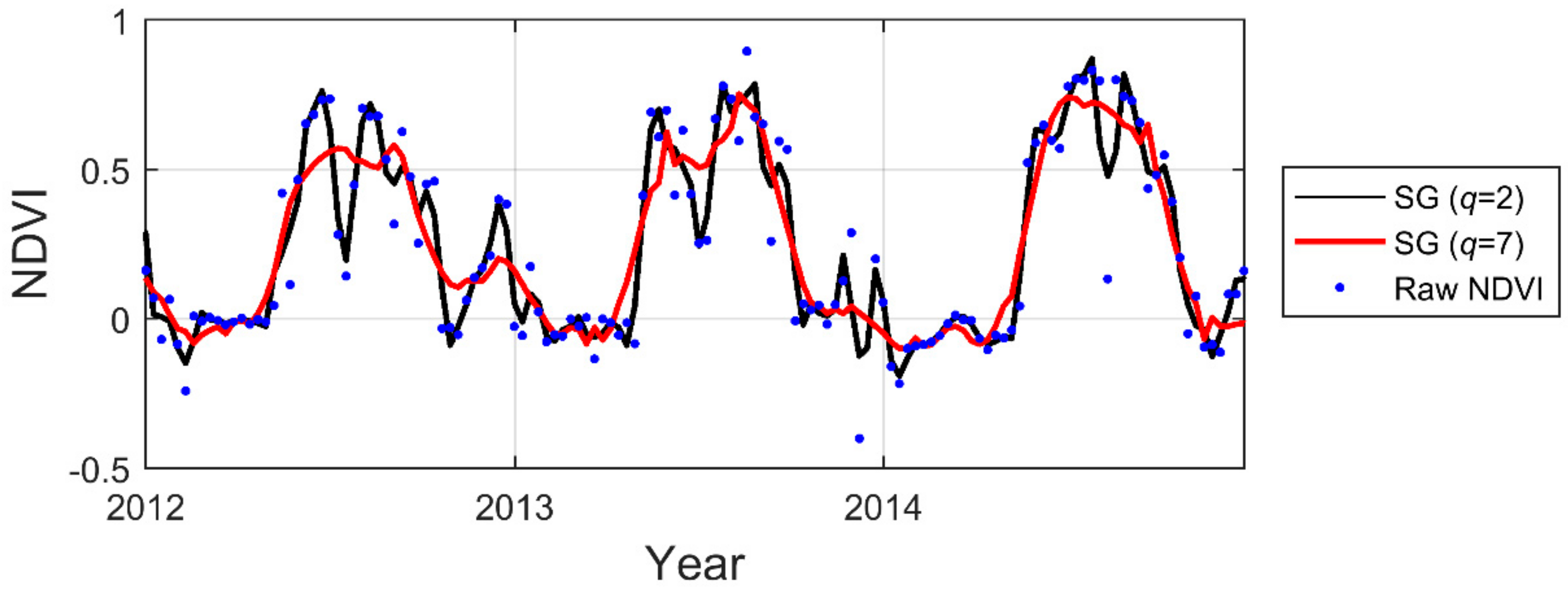
Figure 4.
Examples of LOESS (LO) smoothing with different window sizes, .
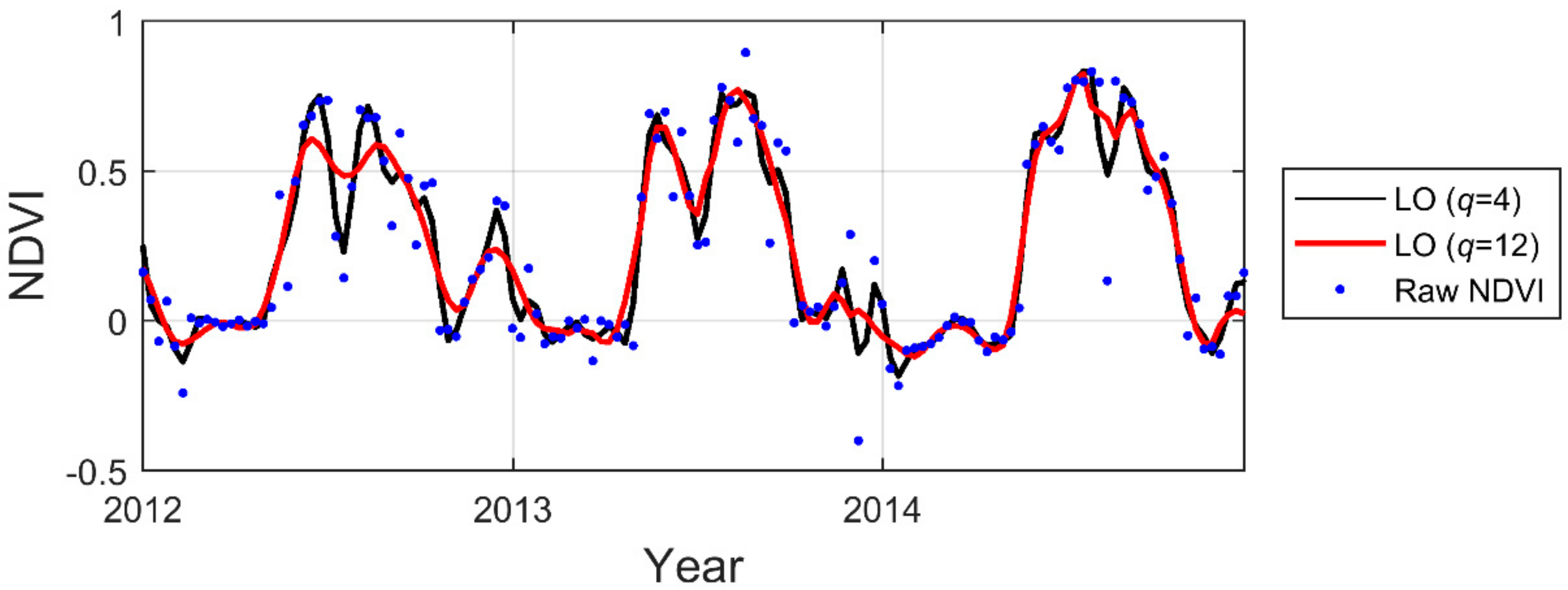
Figure 5.
Examples of spline function smoothers (SP) with different smoothing parameters (p) and cross validation (SPCV).
Figure 5.
Examples of spline function smoothers (SP) with different smoothing parameters (p) and cross validation (SPCV).

Figure 6.
Examples of spline functions with cross validation (SPCV) and different stiffness strength .
Figure 6.
Examples of spline functions with cross validation (SPCV) and different stiffness strength .
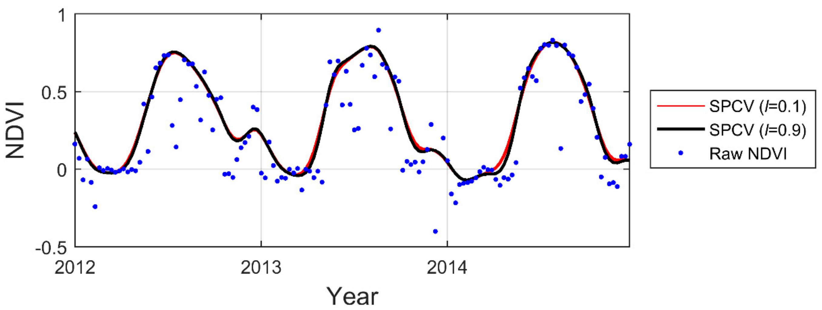
Figure 7.
Examples of least-squares fits to asymmetric Gaussian (AG) and DL model functions.

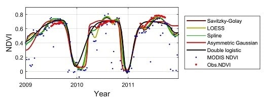
Figure 8.
Smoothed time-series of each method at all test sites based on the settings that provide the minimum RMSE values at Fäjemyr site.
Figure 8.
Smoothed time-series of each method at all test sites based on the settings that provide the minimum RMSE values at Fäjemyr site.
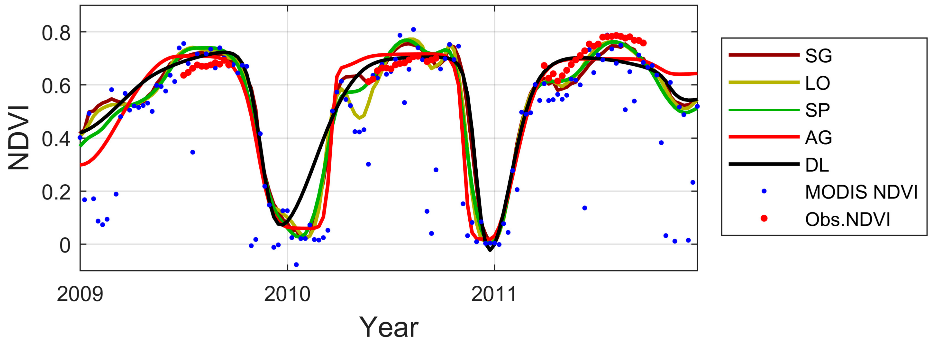
Figure 9.
Boxplot of the Spearman’s rank correlation coefficient between elevation in the Ammar region and ten years’ average vegetation phenology parameters, estimated from smoothed MODIS NDVI time-series by each method with different settings for the period 2001–2010. The black squares in SG, LO and SP are generated from auto-selecting parameters by CV. Note: inverted y-scale on EOS, LOS and SI: lowest negative ρ at the top of the graphs, and the outliers are not shown.

Figure 10.
Maps of start of the season (SOS), end of the season (EOS), length of the season (LOS) and small seasonal integral (SI) for the Ammar region, generated using the optimized settings of DL.
Figure 10.
Maps of start of the season (SOS), end of the season (EOS), length of the season (LOS) and small seasonal integral (SI) for the Ammar region, generated using the optimized settings of DL.


Table 1.
Ground-based spectral observation sites and flux tower sites (more information available in Table S1).
Table 1.
Ground-based spectral observation sites and flux tower sites (more information available in Table S1).
| Site | Latitude | Longitude | Elevation a.s.l. (m) | Spectral Sensor Footprint Area (m2) | Biome | Year of Spectral (CO2 Flux) Data |
|---|---|---|---|---|---|---|
| Abisko Delta | 68.36 | 18.80 | 340 | 2000 | Deciduous forest | 2009–2011 |
| Abisko Stordalen | 68.36 | 19.05 | 360 | 2000 | Sub-arctic mire | 2009–2011 |
| Fäjemyr * | 56.27 | 13.55 | 140 | 3000 | Permanent wetlands | 2009–2011 (2005–2009) |
| Zackenberg * | 74.48 | −20.56 | 1300 | 10,000 | Arctic mire | 2008–2010 (2008–2009) |
| Hyytiälä * | 61.85 | 24.29 | 170 | 7000 | Coniferous forest | 2009–2012 (2005–2012) |
| Norunda Clear-cut | 60.09 | 17.47 | 70 | 300 | Coniferous forest (Clear-cut in 2009) | 2011–2014 |
| Norunda Forest * | 60.09 | 17.48 | 70 | 1500 | Coniferous forest | 2010–2012 (2005–2007) |
| Sudan Barah | 13.82 | 30.36 | 500 | 10,000 | Grassland | 2008–2010 |
| Sudan Dilling | 11.86 | 29.72 | 720 | 10,000 | Grassland | 2008–2009 |
| Sudan Demokeya | 13.27 | 30.49 | 530 | 10,000 | Cropland | 2008–2009 |
* Ground-based spectral observation sites with flux measurements.
Table 2.
Number of parameters of each smoothing method. Altogether, 987 simulations were made for each test site.
Table 2.
Number of parameters of each smoothing method. Altogether, 987 simulations were made for each test site.
| Smoothing Method | Upper-Envelope Iterations () | Upper-Envelope Strength () | Smoothing Parameter (/) | Stiffness Strength () | Total Number of Settings |
|---|---|---|---|---|---|
| SG | 1–3 | 1–10 | 2–7 | - | 126 |
| LO | 1–3 | 1–10 | 4–12 | - | 189 |
| SP | 1–3 | 1–10 | (−1)–1 | 0.1–0.9 | 630 |
| DL | 1–3 | 1–10 | - | - | 21 |
| AG | 1–3 | 1–10 | - | - | 21 |
Note: : number of iterations of upper-envelope, : adaption strength of upper-envelope iterations (only valid for ), : half window size, : smoothing parameter, : adaption strength of spline stiffness.
Table 3.
The ten sites’ average of minimum, median and range of root mean squared error (RMSE) between smoothed moderate-resolution imaging spectroradiometer (MODIS) derived normalized difference vegetation index (NDVI) from all settings of each smoothing algorithm and ground measured NDVI.
Table 3.
The ten sites’ average of minimum, median and range of root mean squared error (RMSE) between smoothed moderate-resolution imaging spectroradiometer (MODIS) derived normalized difference vegetation index (NDVI) from all settings of each smoothing algorithm and ground measured NDVI.
| Statistic | SG | LO | SP | AG | DL | Average |
|---|---|---|---|---|---|---|
| Minimum | 0.063 | 0.062 | 0.064 | 0.066 | 0.069 | 0.065 |
| Median | 0.076 | 0.075 | 0.085 | 0.076 | 0.077 | 0.078 |
| CV | 0.077 | 0.077 | 0.076 | - | - | - |
| Range | 0.069 | 0.068 | 0.071 | 0.038 | 0.035 | 0.056 |
Note: the RMSE between raw MODIS NDVI and ground measured NDVI is 0.142.
Table 4.
The four sites’ average maximum, median and range of between smoothed MODIS NDVI from all settings of each smoothing algorithm and ground measured GPP.
Table 4.
The four sites’ average maximum, median and range of between smoothed MODIS NDVI from all settings of each smoothing algorithm and ground measured GPP.
| Statistic | SG | LO | SP | AG | DL | Average |
|---|---|---|---|---|---|---|
| Maximum | 0.635 | 0.635 | 0.658 | 0.673 | 0.603 | 0.641 |
| Median | 0.488 | 0.498 | 0.505 | 0.555 | 0.503 | 0.510 |
| CV | 0.453 | 0.528 | 0.534 | - | - | - |
| Range | 0.313 | 0.245 | 0.243 | 0.215 | 0.165 | 0.236 |
Note: the between raw MODIS NDVI and ground measured NDVI is 0.338.
Table 5.
The median of ρ between elevation and vegetation phenology parameters extracted by each smoothing algorithm and all settings. Numbers in parenthesis are generated from auto-selecting parameters by CV.
Table 5.
The median of ρ between elevation and vegetation phenology parameters extracted by each smoothing algorithm and all settings. Numbers in parenthesis are generated from auto-selecting parameters by CV.
| Phenology Parameter | SG | LO | SP | AG | DL |
|---|---|---|---|---|---|
| SOS | 0.682 (0.335) | 0.715 (0.786) | 0.693 (0.875) | 0.887 | 0.891 |
| EOS | −0.585 (0.002) | −0.637 (−0.667) | −0.668 (−0.753) | −0.767 | −0.785 |
| LOS | −0.732 (−0.130) | −0.765 (−0.788) | −0.776 (−0.861) | −0.873 | −0.874 |
| SI | −0.518 (−0.082) | −0.566 (−0.587) | −0.558 (−0.569) | −0.630 | −0.655 |
© 2017 by the authors. Licensee MDPI, Basel, Switzerland. This article is an open access article distributed under the terms and conditions of the Creative Commons Attribution (CC BY) license (http://creativecommons.org/licenses/by/4.0/).
Share and Cite
MDPI and ACS Style
Cai, Z.; Jönsson, P.; Jin, H.; Eklundh, L. Performance of Smoothing Methods for Reconstructing NDVI Time-Series and Estimating Vegetation Phenology from MODIS Data. Remote Sens. 2017, 9, 1271. https://doi.org/10.3390/rs9121271
AMA Style
Cai Z, Jönsson P, Jin H, Eklundh L. Performance of Smoothing Methods for Reconstructing NDVI Time-Series and Estimating Vegetation Phenology from MODIS Data. Remote Sensing. 2017; 9(12):1271. https://doi.org/10.3390/rs9121271
Chicago/Turabian StyleCai, Zhanzhang, Per Jönsson, Hongxiao Jin, and Lars Eklundh. 2017. "Performance of Smoothing Methods for Reconstructing NDVI Time-Series and Estimating Vegetation Phenology from MODIS Data" Remote Sensing 9, no. 12: 1271. https://doi.org/10.3390/rs9121271
Note that from the first issue of 2016, this journal uses article numbers instead of page numbers. See further details here.