Monitoring Annual Urban Changes in a Rapidly Growing Portion of Northwest Arkansas with a 20-Year Landsat Record

Abstract

Northwest Arkansas has undergone a significant urban transformation in the past several decades and is considered to be one of the fastest growing regions in the United States. The urban area expansion and the associated demographic increases bring unprecedented pressure to the environment and natural resources. To better understand the consequences of urbanization, accurate and long-term depiction on urban dynamics is critical. Although urban mapping activities using remote sensing have been widely conducted, long-term urban growth mapping at an annual pace is rare and the low accuracy of change detection remains a challenge. In this study, a time series Landsat stack covering the period from 1995 to 2015 was employed to detect the urban dynamics in Northwest Arkansas via a two-stage classification approach. A set of spectral indices that have been proven to be useful in urban area extraction together with the original Landsat spectral bands were used in the maximum likelihood classifier and random forest classifier to distinguish urban from non-urban pixels for each year. A temporal trajectory polishing method, involving temporal filtering and heuristic reasoning, was then applied to the sequence of classified urban maps for further improvement. Based on a set of validation samples selected for five distinct years, the average overall accuracy of the final polished maps was 91%, which improved the preliminary classifications by over 10%. Moreover, results from this study also indicated that the temporal trajectory polishing method was most effective with initial low accuracy classifications. The resulting urban dynamic map is expected to provide unprecedented details about the area, spatial configuration, and growing trends of urban land-cover in Northwest Arkansas.

1. Introduction

More than half of the world’s population currently resides in urban areas, and the coming decades are predicted to bring further profound changes to the size and spatial distribution of the global population [1]. From their earliest beginnings, city landscapes have left an indelible mark on the Earth [2]. Even though they are considered the engines of economic development and social transformations, rapid urbanization is creating tremendous stresses on the environment, natural resources, and public health not only within the city boundaries, but also in areas extending well beyond them [3,4,5]. Urban growth is a major indicator of environmental quality and ecosystem health [6], by driving long-lasting wildlife habitat degradation [7], altering genetic diversity [8], influencing changes in biogeochemistry [9], exacerbating urban heat island effects [10], stressing the disease burden [4], increasing air pollution, and also increasing greenhouse gas emissions [11].

As the size and number of cities continues to grow, their impacts on the coupled natural and human systems will become even more apparent [12]. The rate and trends of these changes in the urbanized areas and their consequences warrant careful consideration and planning by managers and policy makers to promote informed decisions that balance the positive economic effects of urban expansion with their degrading effects. Thus, accurate, consistent, and timely data on trends in urban growth are needed for assessing current and future needs. Unfortunately, for large parts of the world, this type of information is unavailable. Although traditional field-based approaches can provide detailed and spatially disaggregated information on urban change, they are not labor and cost effective, and thus have limited spatial coverage and temporal frequency [13]. Remote sensing provides us with an opportunity to systematically track the magnitude and trends of urbanization. Several land-use/land-cover (LULC) datasets that contain urban layers have been developed using remote sensing, such as the 500-m Moderate Resolution Imaging Spectroradiometer global urban extent map [14], 30-m National Land Cover Database Percent Developed Imperviousness [15], and the 30-m Finer Resolution Observation and Monitoring-Global Land Cover [16]. However, large complex national databases are most accurate when used to support regional and national analysis rather than local applications [17]. In addition, most products lack sufficient temporal resolution and are not useful in characterizing the urban spatial dynamics over a long-term period.

Traditional techniques designed for multi-temporal change analysis can be broadly categorized into temporal trajectory analyses and post-classification comparisons. Temporal trajectory analysis involves the detection of landscape or ecological processes from the time series curves that are constructed from spectral values or vegetation indices of high-temporal-frequency satellite data [18,19,20]. This method is especially useful in discriminating slow-evolving changes from abrupt events. However, the change detection results are sensitive to site-specific control parameters that are used to fine tune the trajectory, and thus require additional calibration efforts. Moreover, updating maps when new images are available requires the reanalysis of the whole temporal trajectory, which is not only computationally intensive, but may alter the original results because the trajectory trend will be changed with the inclusion of new values in the time series. Post-classification comparison is another multi-temporal change detection technique, which classifies the images at each date independently to retrieve the land-cover change information. It is easy to implement and flexible in updating, but the change detection accuracy is highly dependent on the classification performance at each date [21]. Thus, errors arise from single-date image classification due to clouds, speckle noise in images, and classification uncertainties that can get accumulated and become more critical as longer time series of images are involved. In this study, a recently developed change detection method [22] that integrates the robust change detection strength of the temporal trajectory approach and the flexible advantage of post-classification comparison was applied to characterize urban growth from multi-temporal Landsat images in Northwest Arkansas (NWA) for the past two decades.

NWA is diverse in landscape types and is the fastest growing metropolitan area in Arkansas [22], which makes it a perfect choice for engineering and implementing this new methodology to detect urban growth. A previous study using this methodology was applied to urban areas in Beijing. The results from that study demonstrated the reliability and usefulness in modeling and monitoring the effects of urban planning [23]. However, because of the different cultural and settlement patterns along with the variations in the urban morphology between Beijing and NWA, the applicability of this approach in a U.S. metropolitan statistical area remains uncertain. Urban landscapes in Beijing are characterized by highly concentrated hard surfaces, and most built-up patches are separated from green spaces, which make it possible to identify them as pure urban or non-urban pixels on a 30 m resolution image. In contrast, cities in NWA often have buildings interspersed with open green areas. As a result, their composite spectral responses can introduce many uncertainties as well as add confusion in long-term change detection. Thus, the objectives of this study were to:

• Test our algorithm in a highly heterogeneous urban landscape to map the urban extent on a yearly basis;
• Quantify the patterns and trends of urban growth in NWA based on the generated urban extent maps.

2. Materials and Methods

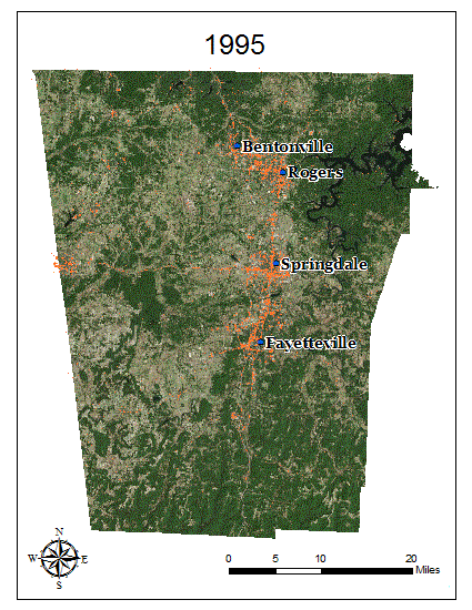
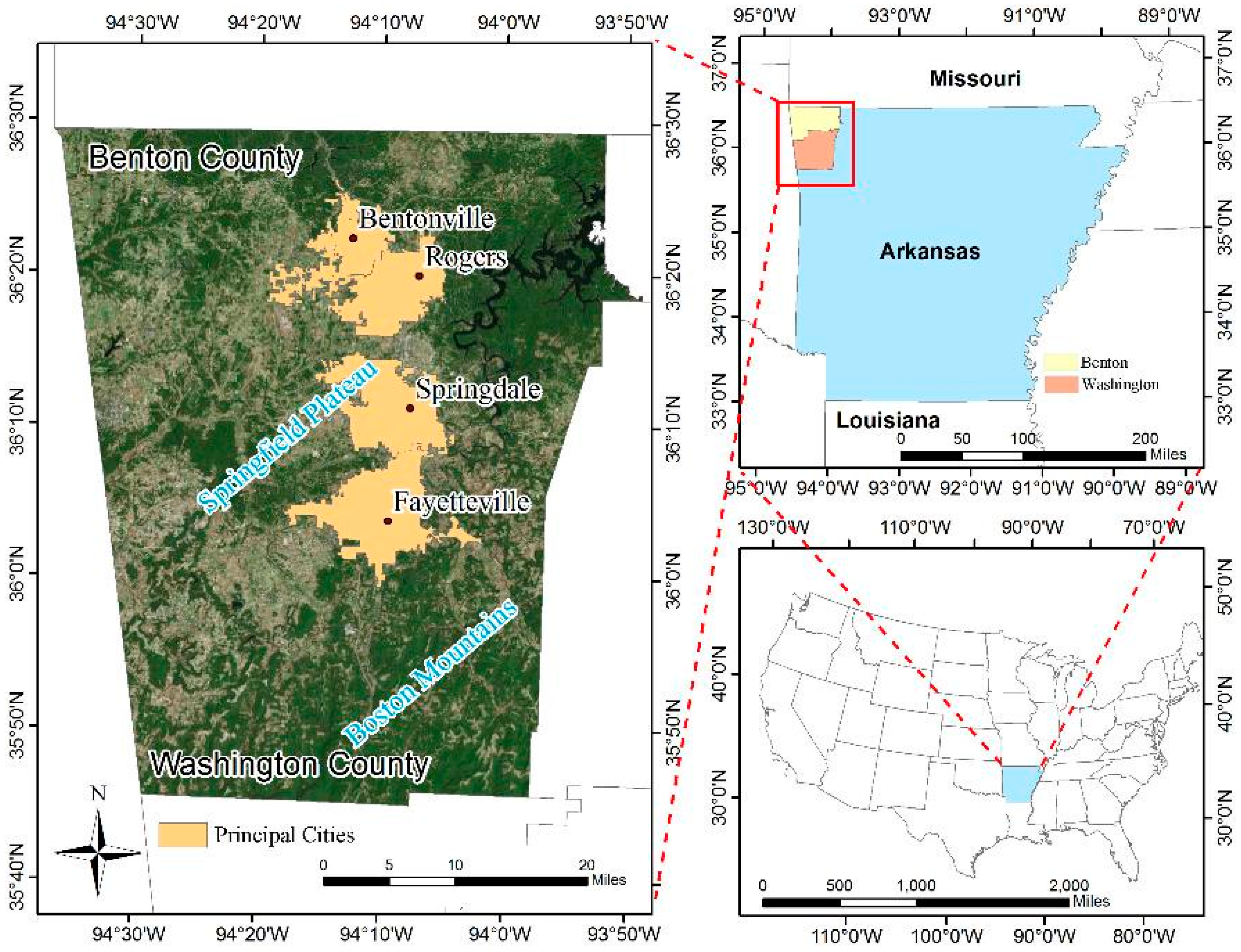
2.1. Study Area

Northwest Arkansas (NWA) is one of the most dynamic metropolitan statistical areas (MSA) in the U.S. [24]. While NWA is comprised of four counties (Benton, Carroll, Madison, and Washington), this study focuses on the two most heavily populated counties of NWA (Benton and Washington). Within these two counties are four of the state’s fastest growing cities, specifically Bentonville, Rogers, Springdale, and Fayetteville oriented in a north to south linear direction (Figure 1). These cities are bounded by the rugged Boston Mountains to the east and south while the gently rolling Springfield Plateau characterizes the western portion of both counties.

Since the mid-1990s, considerable urban expansion within NWA has been driven primarily by the influences of Wal-Mart Stores, Inc. (the world’s largest retailer), Tyson Foods (the nation’s largest processor of chicken, beef, and pork products), J.B. Hunt Transport Services, Inc. (one of the nation’s largest freight shipping companies), and over 1300 suppliers and vendors drawn to the region by these large businesses, NWA’s economic climate, and its geographical location [25]. These three companies alone boasted an estimated net sales of over 500 billion dollars in 2014 [26,27,28]. In addition to these three economic drivers, the University of Arkansas, located in Fayetteville, has contributed to the continual urban expansion within NWA through regular increases in student enrollment rates and is considered to be the seventh fastest growing public university in the nation [29]. During the period between 1980 and 2015, the total population in the state of Arkansas increased by 30%, doubling the population in Washington County and tripling the population in Benton County (Figure S1).

2.2. Image Acquisition and Preprocessing

Changes in land-cover were examined using Landsat data records from 1995 to 2015 (

Table 1. Landsat acquisition date and sensor type.

	Year	Date	Sensor	Cloud Cover
1	1995	23 August	L5-TM	0.00%
2	1996	2 March	L5-TM	0.00%
3	1997	28 August	L5-TM	0.00%
4	1998	24 March	L5-TM	0.00%
5	1999	18 August	L5-TM	0.00%
6	2000	4 August	L5-TM	0.00%
7	2001	22 July	L5-TM	0.00%
8	2002	11 September	L5-TM	0.00%
9	2003	16 October	L5-TM	0.00%
10	2004	2 October	L5-TM	0.00%
11	2005	19 September	L5-TM	0.00%
12	2006	5 August	L5-TM	0.00%
13	2007	20 May	L5-TM	0.00%
14	2008	27 September	L5-TM	0.00%
15	2009	7 April	L5-TM	0.00%
16	2010	31 July	L5-TM	0.00%
17	2011	3 August	L5-TM	0.00%
18	2013	9 September	L8-OLI	0.03%
19	2014	20 March	L8-OLI	0.05%
20	2015	14 August	L8-OLI	0.25%

). NWA lies entirely within Landsat path 26 row 35. Images were primarily collected for leaf-on season conditions, from mid-March through mid-October, to ensure the strongest spectral contrast between urban areas and green vegetation. Some images were chosen outside of the ideal time of year due to excessive cloud cover. For each year, one cloud-free or mildly contaminated image was selected to build the time series. In this study, both Landsat Top of Atmosphere products and Landsat Surface Reflectance Climate Date Records were acquired from the U.S. Geological Survey (except the year 2012). All images had been processed to L1T level (i.e., passed the corrections of topography and radiation). For the atmospheric correction with the Surface Reflectance datasets, Landsat 4–5 TM and Landsat 7 ETM+ were processed uniformly with the Landsat Ecosystem Disturbance Adaptive Processing System [30] and Landsat 8 Operational Land Imager (OLI) were processed with the Fast Line-of-Sight Atmospheric Analysis of Spectral Hypercubes algorithm [31]. Landsat 5 Thematic Mapper (TM) imagery was used for the years 1995 to 2011 and Landsat 8 OLI imagery was used for years 2013 to 2015. The year 2012 was omitted from the study due to the Landsat 7 Scan Line Corrector failure in 2003, the decommission of Landsat 5 due to multiple mechanical failures in 2012, and the unavailable data of Landsat 8 due to its 2013 launch date.

The time series of Landsat Surface Reflectance image collection was used to calculate spectral indices that have been proven to be useful in improving the classification performance, including: Normalized Difference Vegetation Index (NDVI) to help distinguish between vegetation and non-vegetation [32], Normalized Difference Built-up Index (NDBI) to better visualize built up impervious surfaces usually associated with urban areas [33], Built-up Index (BUI) [33], and Principal Component Analysis (PCA). The first three principal components from PCA were used. In addition, Landsat Top of Atmosphere reflectance images were used to calculate the Tasseled Cap Transformation for Landsat TM [34] and Landsat 8 OLS [35]. The brightness, greenness, and wetness from Tasseled Cap Transformation were included. The nine new transformations, in conjunction with the original six bands, were compiled together and used in the classifications

NDVI = (ρNIR − ρRed)/ρNIR + ρRed)

(1)

NDBI = (ρSWIR − ρNIR)/(ρSWIR + ρNIR)

(2)

BUI = NDVI − NDBI

(3)

where ρRed, ρNIR, and ρSWIR are the surface reflectance values of the red band (600–690 mm), near-infrared band (760–900 mm), and shortwave-infrared band (1550–1750 mm), respectively.

2.3. Classification System and Classification Sample Selection

Five land-cover types encompassing the majority of the NWA landscape were considered in the classification and are as follows:

• High-intensity urban: a highly developed area where impervious surfaces account for 80% to 100% of the total cover, mostly containing commercial and industrial property that appears to have a higher reflectance value than the low-intensity urban [36,37];
• Low-intensity urban: a less developed area where impervious surfaces account for 50% to 80% of the total cover, mostly containing residential areas such as neighborhoods, apartments, and roadways [36,37]. Dirt and gravel roads were not included in either of the urban classes due to their spectral signatures being similar to bare soils, harvested croplands, and water coastlines. To minimize confusion, only paved roads were included in the classification scheme;
• Agriculture/Pasture/Bare Lands: open areas of crops planted by farmers, grass, or other short vegetative growth in fields and bare patches of lands that lack intense vegetation. In NWA, due to Tyson Foods Inc., there are many pasture lands that are dedicated to the cultivation and harvest of poultry and beef. Agriculture in NWA is not as common as it is in the rest of Arkansas, but is present in the region. Bare lands are areas that have not been used for agriculture or pasture for animals, and are usually land stocks for urban expansion;
• Forest: an area that is dominated mostly by dense tree cover. NWA contains a number of national forests and parks, including the Ozark National Forest. These forested areas are, for the most part, very homogeneous in nature, containing about 80% to 100% tree cover with very little gaps. These gaps would be classified into the Agriculture/Pasture/Bare lands classification;
• Water: includes lakes, ponds, rivers, streams, and creeks that are visually identifiable on the Landsat imagery.

Training samples were collected through visual interpretation of the 15-band stacked Landsat imagery. The locations of those training samples were consistent throughout the study time period and their labels were interpreted for each year. Very high resolution Google Earth imagery, Bing Maps, and the 1-m resolution U.S. Department of Agriculture National Agriculture Imagery Program (NAIP) [38] were used to verify homogeneity in training sample locations. It should be noted that a critical prerequisite for good classification performance is that the training samples be representative in that they cover the whole spectral range of the land-cover types. To achieve this goal, the following criteria were used:

• More than 30 samples required for each class, which is the standard number of minimum samples necessary for accurate classification based on the sample size formula as recommended by [39].
• Samples needed to be greater than four pixels in size.
• Samples needed to be homogeneous in nature.

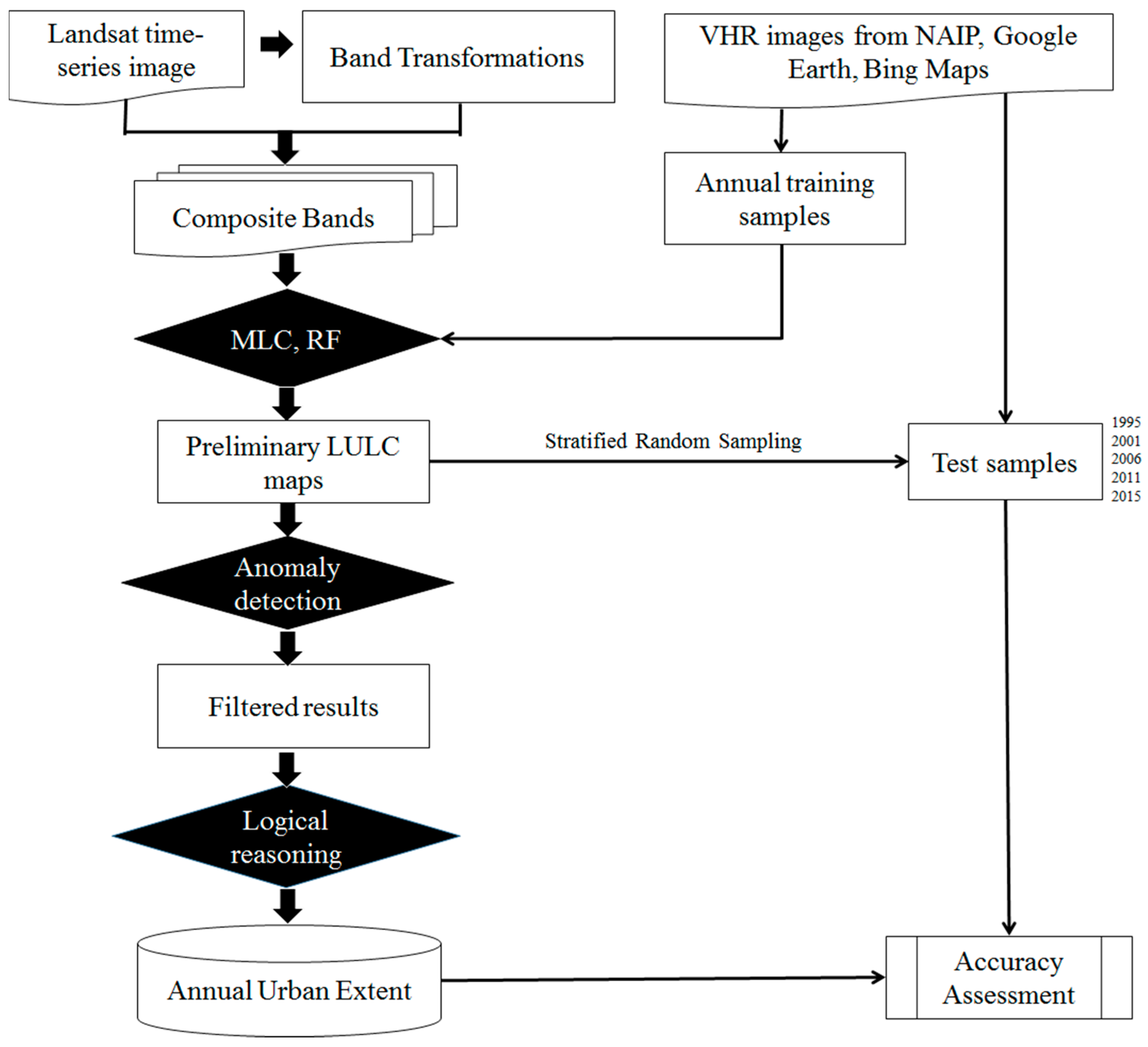
2.4. Classification Framework

The biggest obstacle with post-classification change detection techniques are the propagated errors that arise from independent single-date classifications. For better change detection results, refinements are needed to stabilize year-to-year variation in classification labels not associated with actual land-cover changes. This issue was addressed via the Temporal Trajectory Polishing method, which involves two steps: anomaly detection and label adjustment in the trajectories of classified LULC change followed by logic reasoning ([23]; Figure 2).

2.4.1. Preliminary Classification

For each year, preliminary classifications were first performed with the Maximum Likelihood Classifier (MLC) and Random Forest classifier (RF) using the combined six raw spectral bands and nine spectral indices. The MLC is a parametric method widely used as a reference for its computational simplicity and robustness. All classes were assigned to have the equal prior probability and no pixel would be rejected for class assignment. The RF classifier is a machine-learning algorithm that combines the results of many (thousands) decision trees [40], and is often praised for its overall performance, as well as robustness to noise [41]. For the RF parameter setting, 500 classification trees were chosen and the number of prediction variables set to the square root of the number of input features. The land-cover files were then regrouped from the original five classes into binary maps containing only urban (High and Low Intensity) and non-urban (Water, Forest, Agriculture/Pasture/Bare Lands) types.

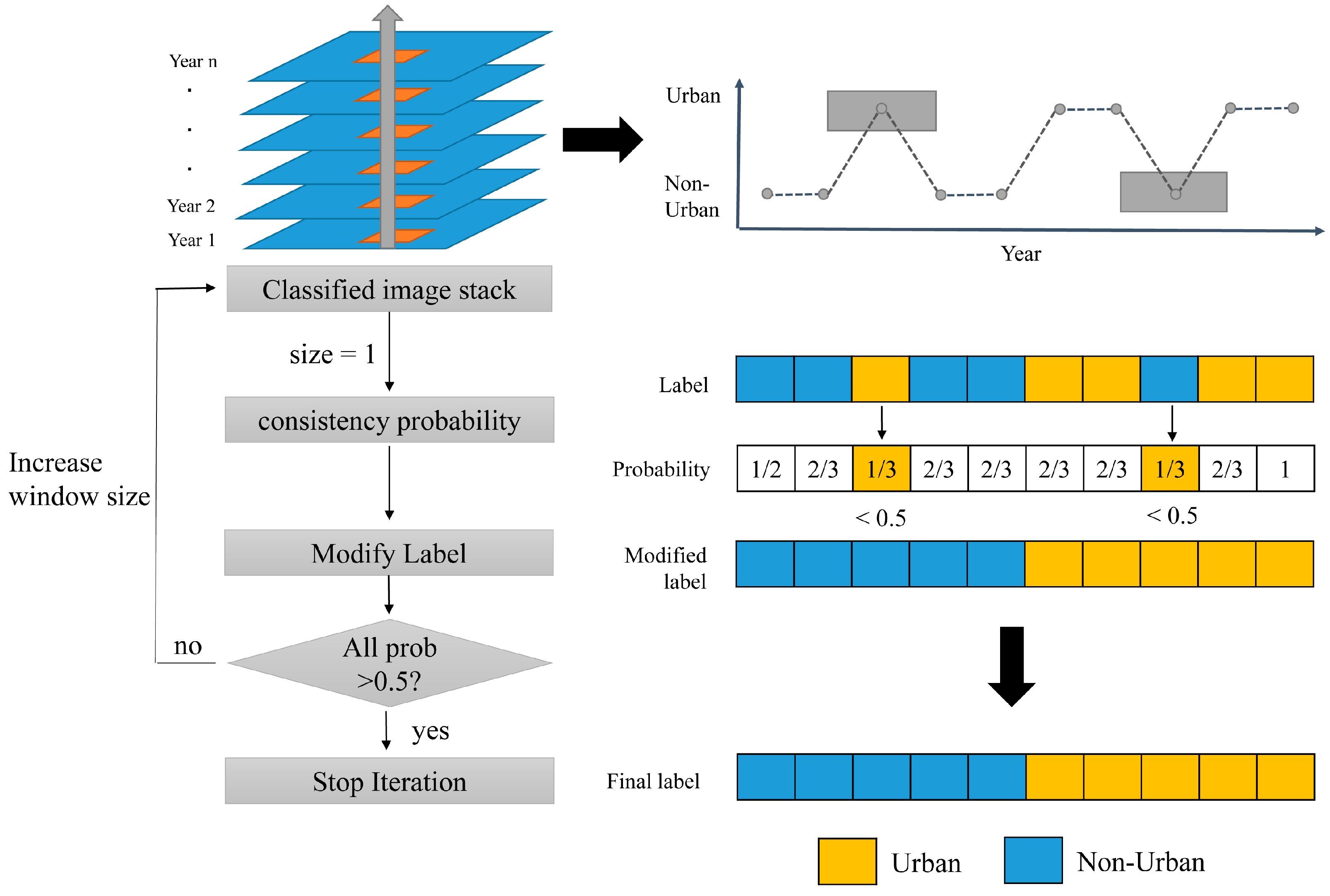
2.4.2. Anomaly Detection and Temporal Filtering

Based on the preliminary binarized urban map, the land-use trajectory was extracted at the pixel level. Land use trajectory is the temporal sequence of LULC classes that are described through classified images assembled in a time-series [42]. Under most circumstances, the transition from non-urban to urban is irreversible. However, due to the various factors affecting the image acquisition, data preprocessing, and classification, errors are unavoidable and can result in a noisy time series trajectory. For example, if a pixel is found labeled as urban in one year, but the adjacent previous and following years are both classified as non-urban, it is likely that this pixel is misclassified for that urban labeled year. Generally speaking, the frequency of land-cover changes should not be high and the anomaly in the time series trajectories can be an indicator of potential misclassification.

To detect and remove the anomaly in the LULC trajectories, an iterative temporal filtering method was used. Specifically, a temporal consistency probability (𝑃_𝑖) was calculated for each year in the trajectory:

$$P_i=\frac{{{\displaystyle \sum }}_{i-T_w}^{i+T_w}con\left(L_j=L_i\right)}{1+2\times T_W}$$

(4)

where Li is the class label of the target year, and Tw is the time window size that starts from 1. Con is a conditional expression that returns 1 when the class labels are the same for the target year and its neighboring year, and vice versa.

As indicated in Figure 3, a low 𝑃𝑖 is more likely to reflect an erroneously classified pixel in the target year and its associated label should be replaced based on the majority of its contiguous neighboring years. Thus, if the probability of the label’s occurrence is less than 0.5, it was different from the designated type inferred from the dominant types in its temporal neighborhoods and then considered as anomalous. The label value will be revised to its opposite accordingly. The window size Tw for defining number of temporal neighborhoods increases gradually from 1, and the whole sequence will be updated after each iteration until all the processed Pi in the temporal trajectory are larger than 0.5. However, it should be noted that because the first year of the study and the last year of the study (the head year and the tail year) lack complete temporal neighborhood information, the filtering may not be as complete as the central years. The implementation of this post-classification step will result in a more consistent and accurate filtered trajectory with fewer spikes caused from impulse noise.

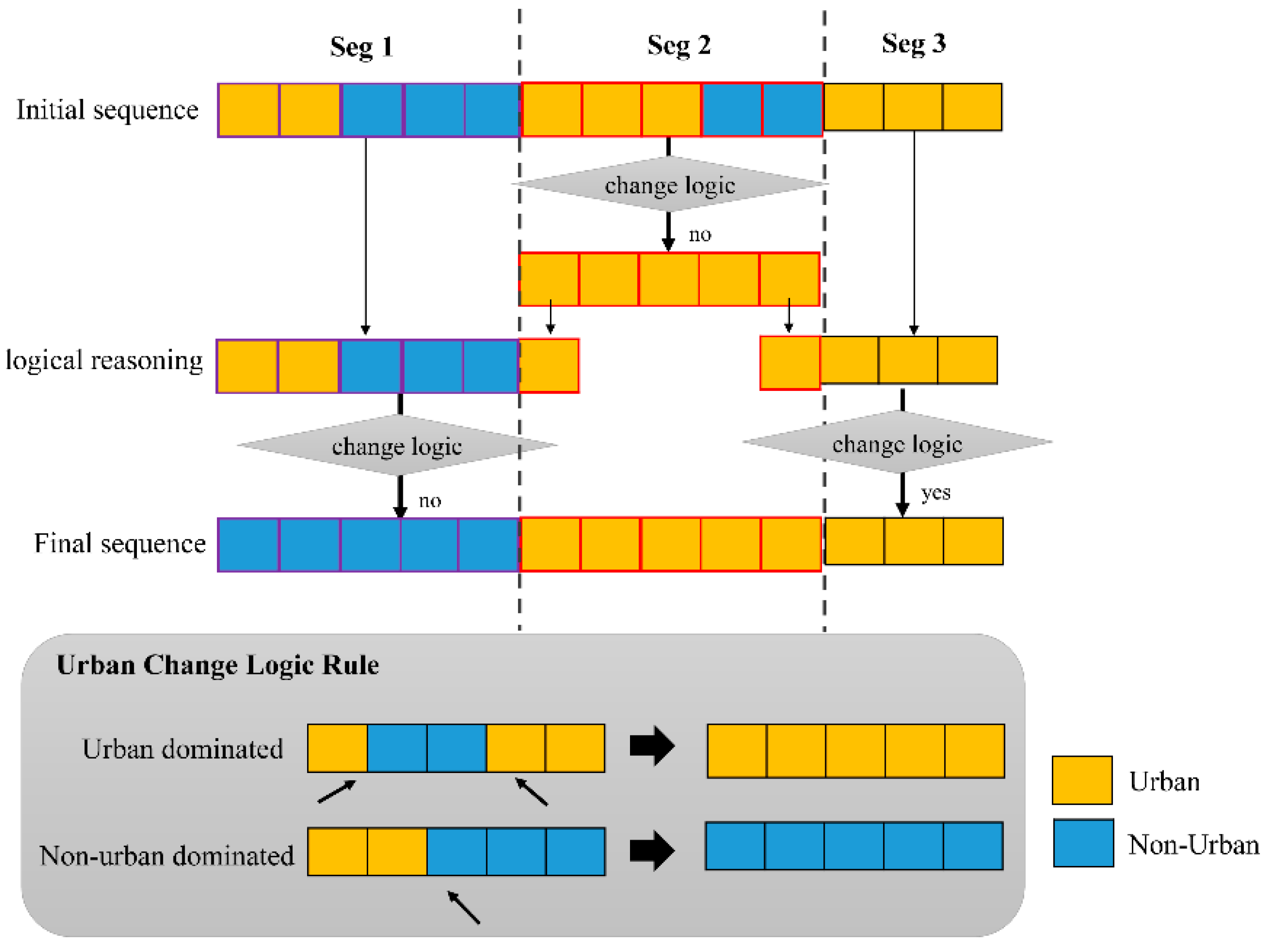
2.4.3. Urban Change Logic Rule

The temporal filtering in Section 2.4.2 can only ensure the consistent classification (urban or non-urban) over temporally consecutive years, whose length was determined iteratively with increased window length. However, it cannot make the whole sequences follow the conversion from non-urban to urban consistently. Therefore, an additional logical reasoning was needed to achieve this goal. For urban environments, the land-use trajectory often follows the temporal non-reversal rule, i.e., land-cover dynamics occur in an irreversible order and the urban impervious pixels cannot revert to non-urban pixels through the remainder of the time series. This leads to the design of the change logic rules with the purpose of modifying the temporal trajectory into a logical order (Figure 4): if non-urban labels happen before urban labels in the original sequence, then it obeys the change logic rule and remains unchanged. If non-urban labels occur after urban labels, the rule is broken. Different strategies were taken to process depending on the dominant land-cover type of the sequence, which is calculated by counting the number of urban and non-urban years within the sequence. If the processed sequence is urban dominated, the unreasonable non-urban labels will be modified to urban. Otherwise, years that contain pixels labeled urban occurring before non-urban labeled pixels would be relabeled to the opposite status.

To achieve the best performance, the urban change logic rules were not directly applied to the whole trajectory because the partial loss of temporal contexts for the head and tail year may impede the deduction of proper logic. Instead, the whole LULC trajectory was divided into three segments, namely the prior segment (Seg 1), the main segment (Seg 2), and the posterior segment (Seg 3). The rules were applied to the main segment first because of its completeness in neighborhood information. The class label of the first and last year of the main segment after logic reasoning were further composited into the prior and posterior segment respectively to aid their logic reasoning. The implementation of this step is to examine the LULC change history at the pixel level and minimize the degree of uncertainty.

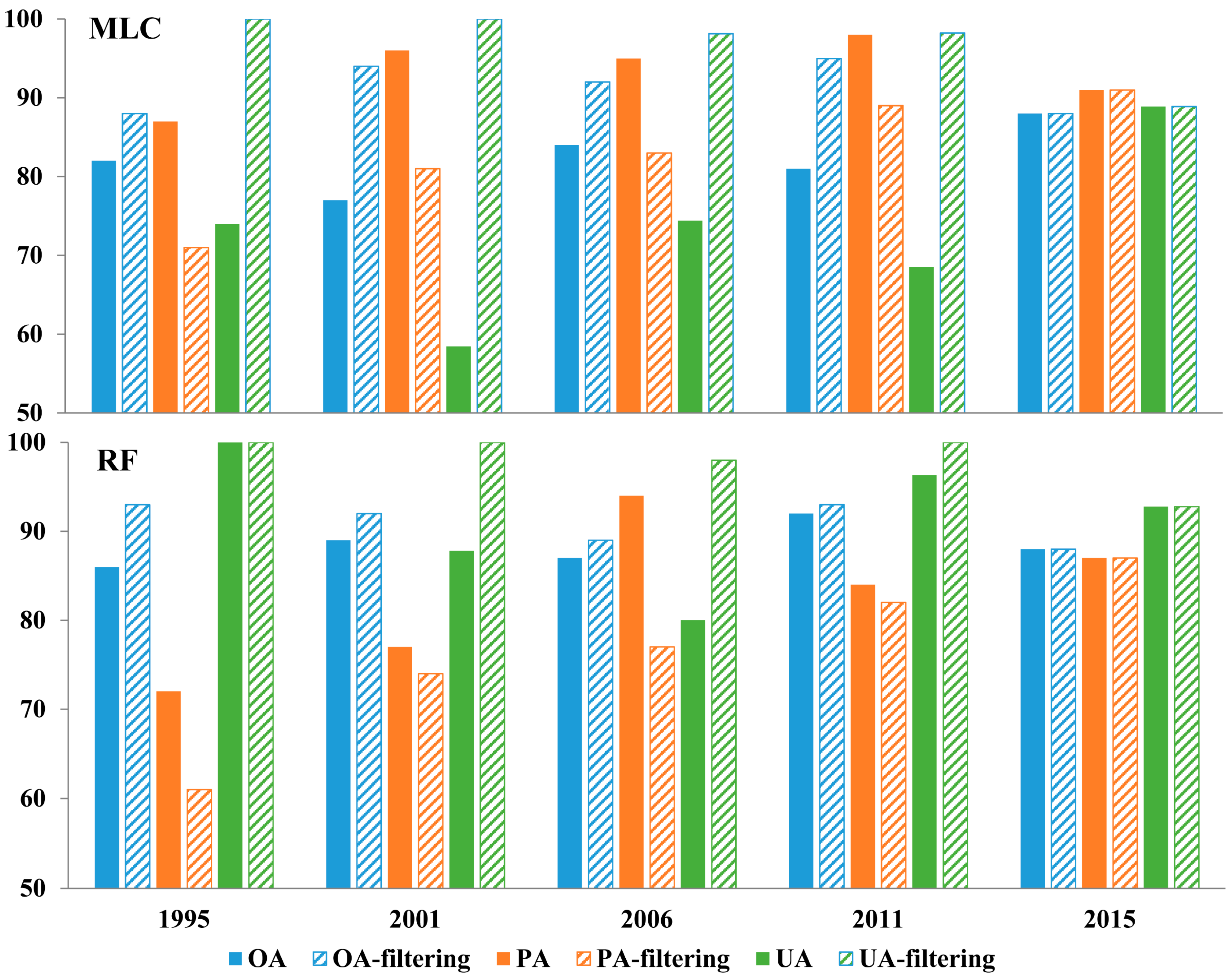
2.5. Accuracy Assessment

The accuracy assessments were conducted in both quantitative and qualitative ways. First, validation samples were collected through a stratified random sampling scheme on the preliminary classification results almost every five years, as well as the starting and ending years (1995, 2001, 2006, 2011, and 2015). The years 2001, 2006, and 2011 were selected because of the National Land Cover Database (NLCD) availability in these years. The years 2006 and 2015 are also the NAIP available years in this region. There were 50 random points generated in the classified urban area and 100 random points for the non-urban areas for each of the test years (Figure S2). The total sample number was calculated based on a well-accepted sample size formula [43] with an expected accuracy of 90% at an allowable error of 5% for a binary-class classification. Considering the importance of the urban category within the objectives of this project, we did not follow the area proportion assignment rule that would make the sample size for urban very small. Instead, we adjusted the number of urban samples to 50 according to the rule of thumb proposed by [44,45]. For the five validation years, a total of 750 points were generated, which were then visually interpreted and labeled one at a time against a combination of NAIP (for year 2006, 2015), Google Earth (for all validation years), and Bing Maps imagery (for year 2015). All of the validation samples were cross-checked by team members for quality control. When samples were not easy to interpret, quality controllers flagged them and the points were visually revisited for interpretation until a consensus was achieved. A confusion matrix was then created for each test year and associated accuracy measures were generated, including the overall accuracy (OA), Kappa, producer’s accuracy (PA), and user’s accuracy (UA) [46]. These accuracy measures use and summarize different information contained in the confusion matrix. Overall accuracy accounts for the overall proportion of area correctly classified. Producer’s accuracy measures errors of omission while user’s accuracy measures errors of commission.

Results were then visually evaluated by comparing the mapped spatio-temporal pattern of the urban area with the developed area layer included in the NLCD. The NLCD dataset is a Landsat-based 30 m resolution national land-cover dataset, whose years 2001, 2006, and 2011 are directly comparable, and were used for comparison to this product. NLCD 2001, NLCD 2006, and NLCD 2011 were selected because they covered the study period for comparison. The NLCD classification scheme was adapted from the Anderson Land Cover Classification System with eight Level I classes and 16 Level II classes. Both NLCD 2001 and NLCD 2006 were accomplished using decision tree classifiers and their accuracy assessment was completed through a set of fixed location stratified randomly selected samples that were interpreted based on multi-temporal high resolution digital imagery. The reported Level I class overall accuracies were 85% in 2001 and 84% in 2006 [47]. For the two urban classes (class 23: developed medium intensity and class 24: developed high intensity) that match with our urban definition, their producer’s accuracies were 75% for class 23 and 81% for class 24 in NLCD 2001 and 80% for class 23 and 26% for class 24 in NLCD 2006. Their user’s accuracies were 67% and 87% in NLCD 2001 and 69% and 83% in NLCD 2006 [47]. NLCD 2011 was completed by spatially integrating NLCD 2006 with the spectral change map of 2006–2011 obtained from the Multi-Index Integrated Change Analysis model [48]. Four Level II classes that fall into the category of developed area were grouped to generate the developed area layer for comparison with the maps.

3. Results

3.1. Accuracy Assessment

The overall accuracies achieved by the benchmark approach MLC for the test years were 82%, 77%, 84%, 81% and 88% (mean: 82%), and were increased to 88%, 94%, 92%, 95% and 88% (mean: 91%) after temporal filtering (Figure 5; Supplementary File 3). Year 2015 reported the same accuracies during the temporal filtering process due to the fact that no post year existed to determine if growth of urban areas was logical. Except for year 2015, the average overall accuracy improvement achieved by the post-classification method was over 10%. The producer’s accuracies for the urban class range were from 87% to 98%, and for the non-urban class range from 68% to 84%. After temporal filtering, the PAs for the urban class dropped about 10% on average, but the improvements of user’s accuracies were over 24%. For the nonparametric classifications based on RF, the average overall accuracy, producer’s accuracy, and user’s accuracies were 88%, 83%, and 91%, and those after filtering were 91%, 76%, and 98%, respectively (Figure 5; Supplementary File 3).

Visual examination showed that temporally filtered maps depicted substantially more spatial heterogeneity of impervious surfaces within urban areas, as opposed to the overestimation of urban lands in the preliminary classification and NLCD developed area layer (Figure 6). In terms of change detection, the initial MLC classification had the worst performance in providing reliable information, as many pixels showed illogical land-cover transition from urban to non-urban. This can severely impair the true change detection accuracy. NLCD data shows more consistent results in urban expansion, as the latest map was generated through the integration of an older land-cover map with the spectral change map. This temporal trajectory polishing method achieved the best results in keeping both the spatial contiguity and temporal consistency.

Overall, RF outperformed in the preliminary classification, and because of its already high accuracies, the improvements with the temporal filtering approach were less significant.

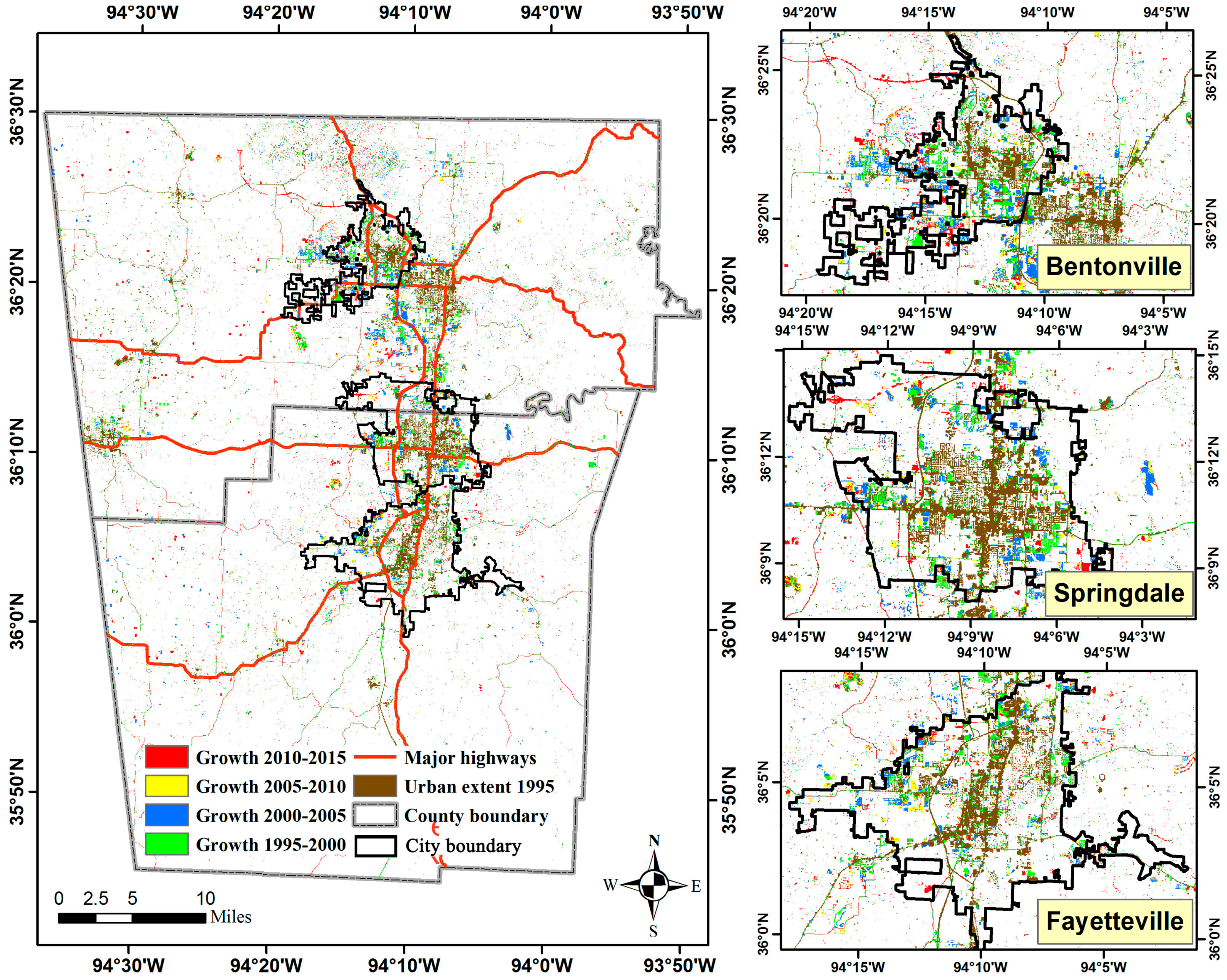
3.2. Urban Expansion in Northwestern Arkansas (NWA)

The urban sprawling is very prominent in all the three cities of NWA, as can be observed from the remote sensing-derived maps (Figure 7; Figure S3).

Bentonville experienced noticeable growth from 1995 to 2000 mainly on the western side of the city in areas lying to the west and south of the major highway. The period between the years 2000 and 2005 was also a period of rapid urban expansion in the Bentonville area, mostly in a westward direction. The period between 2005 and 2010 did not experience as much growth in the Bentonville area save for some developments in the southern Bentonville area and a major added highway in the north running east and west constructed between 2010 and 2015.

Springdale’s most notable urban expansion took place in the years between 1995 and 2000 in the southeastern section of the city limits area as well as the western section of the city limits. The growth in Springdale in the period between 2000 and 2010 was very spatially diverse across the city, with the most notable concentration of urban expansion in the western section of the city. The urban growth in the city of Springdale between 2010 and 2015 can be seen in the far southeastern parts of the city as well as some construction of major roads in the northwest and southwest presumably to allow easier access to the local airport.

The urban expansion in Fayetteville is, overall, very spatially diverse and dynamic during the time period of the study, 1995 to 2015. In the time period between 1995 and 2000 a major highway connection running north and south allowing access to the region was built in the area just south of Fayetteville’s city limits. The greatest urban expansion was experienced in the first half of the study period, between 1995 and 2005, with less intense growth taking place in the latter half of the study, between 2005 and 2015.

4. Discussion

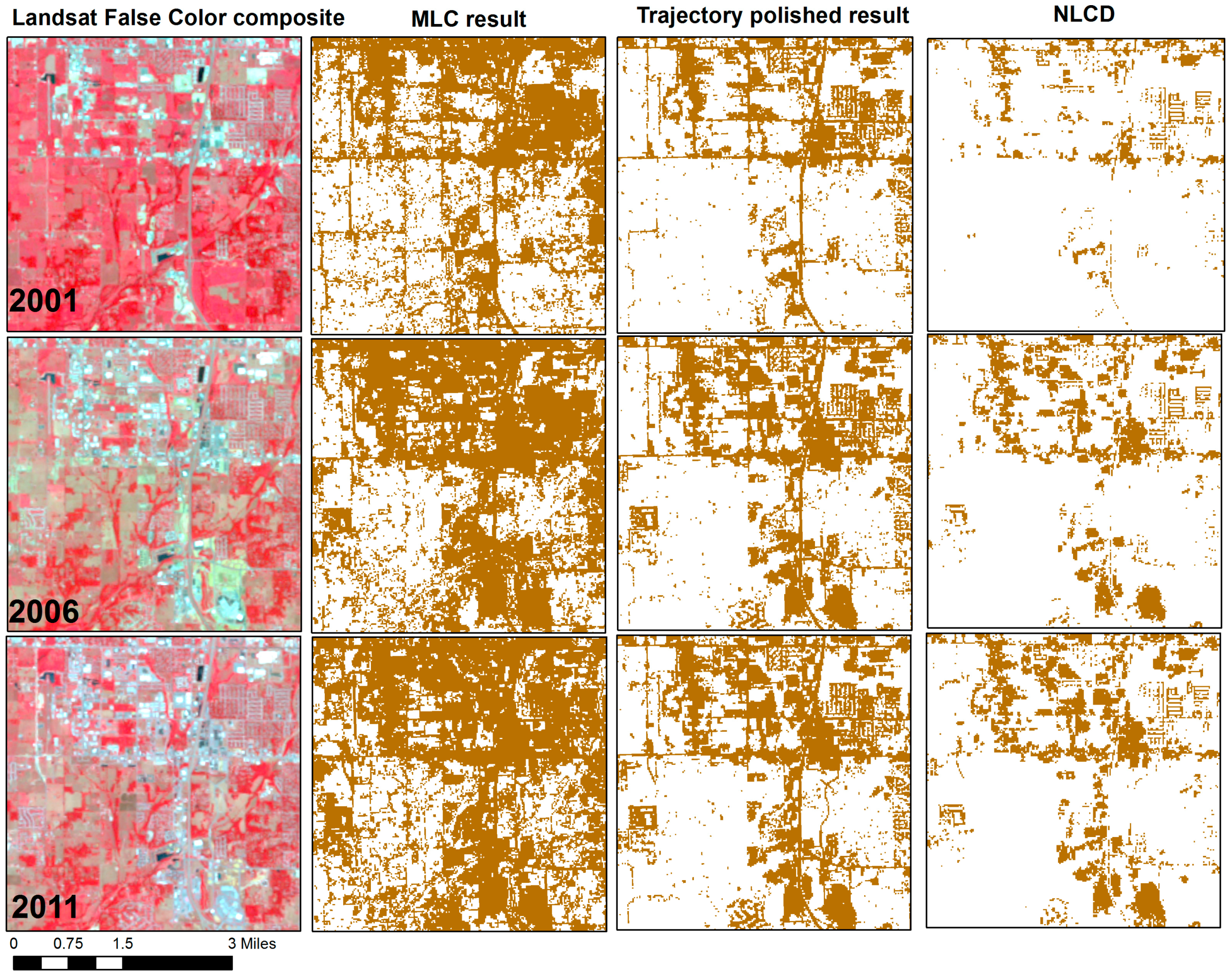
4.1. Pros and Cons of the Temporal Trajectory Polishing Algorithm

The feasibility of using remote sensing for monitoring long-term urban expansion is largely limited by change detection accuracy. Urban landscapes are highly spatially and spectrally heterogeneous due to complicated structures, materials, density, and spatial forms, which make them easier to be confused with other land-cover types based only on their spectral signatures [49]. While it is not easy to accurately map single-date images, it is even more difficult to keep the change detection accuracy high. For the conventional single-date image classification, the RF achieved better overall accuracy than MLC in both initial classifications and post-filtering results by around 5%. This can be mainly attributed to two reasons: (1) MLC relies on assumptions about the data distribution (e.g., normally distributed), whereas the ensemble learning techniques employed by RF do not [50]; (2) MLC is affected less by the selection of input layers than RF. The performance of RF usually is improved with a larger amount of input features because the classification uncertainties are usually negated by using the ensemble of results from many individual trees that are built upon the random selection of input layers [51].

With the temporal trajectory polishing method proposed in this study, the classification results obtained were improved at all dates (except for the last year) for both the parametric MLC and the non-parametric RF, which implies the usefulness of this approach. Improvements were also noticed to be more substantial over the MLC maps, reporting lower accuracies in the initial classifications. This suggests that this method works more effectively with multi-date classifications containing larger amounts of mapping errors. In addition, the comparison with NLCD data proved the superiority of this approach in characterizing the urban landscape details, especially in areas where impervious surface and urban vegetation are highly mixed.

Although the temporal trajectory polishing approach is promising in many ways, one shortcoming is revealed from this case study. Regardless of the improved OA and UA for urban classification, the omission errors for urban classification were elevated after the post-classification process. The higher omission rate was partly due to the finer texture measurements of Landsat 8 OLI imagery and the inconsistency in land-cover characterization between the two sensor types we included: Landsat 5 TM and Landsat 8 OLI [52]. Although both sensors share the same spatial resolution, Landsat 8 imagery has several new features: (1) an enhanced radiometric resolution of 12-bits (16-bits when processed into Level-1 data products) compared to the 8-bit resolution of its predecessor, which improves the spectral record precision and avoids spectral saturation [53]; (2) enhanced signal to noise ratios, almost twice as good as Landsat 7 [54]; (3) narrowed NIR band to avoid the effect of water vapor absorption at 0.825 um. These changes in the instrument’s design allow for a much finer texture and refined spectral range of the OLI bands, especially in the near-infrared bands [52]. Consequently, more land-cover details with slight differences in energy can be characterized by Landsat 8 images. The improved data performance usually results in more satisfactory land-cover classification results, which has been proven by a previous study [52]. For this case study, the OLI image-derived classifications help to better separate the green spaces or bare lands that are intermixed among the built-up pixels when compared with the relatively blurry look of the TM images. However, the test samples interpreted based upon Landsat 5 can hardly reflect the complex urban composition. For instance, a pixel containing a mixture of a high percentage of green vegetation and a low percentage of paved roads could be interpreted as urban on TM images due to its higher spectral reflectance value rather than pure vegetation pixels, but would be labeled as non-urban on an OLI image.

Thus, without better validation samples, it can hardly be concluded that the temporal filtering method will result in higher omission error. For instance, in the previous Beijing case study, consistent improvements were observed over almost all types of accuracy metrics after the temporal polishing [23]. This is because in cities like Beijing, where built-up pixels are relatively purer with less intermixed green spaces, the improvement in classification relies upon the enhanced image sensor and is not as obvious in cities where mixed urban/green space pixels are commonly found.

4.2. Socio-Economic and Environmental Explanations of the Urban Sprawling Patten in NWA

The successful depiction of the dynamic urban expansion in NWA reveals some interesting patterns. The examination of the urban expansion for NWA appears to suggest a reinforcing loop that is being driven by economic and topographic factors.

First of all, Northwest Arkansas saw an annual population increase of approximately 11,328 from 2000 to 2010, indicating an annual growth rate of 3.15% [55]. This annual influx of people into the region may be related to the economic opportunities that are offered due to the location of the four central cities that comprise the NWA. As noted by Gascon and Varley [56], the economic growth of the NWA is unique because it is centered on all four cities, whereas other metropolitan statistical areas typically revolve around one major city. This is supported by a report prepared by the Northwest Arkansas Regional Planning Committee [55] which shows that eight companies within these four cities employ over 1000 individuals each with Wal-Mart leading the group with over 11,000 employees. A result of this has been the rapid development of subdivisions and transportation networks to accommodate the regular influx of people into the region.

Secondly, all four principal cities exhibited a general trend of westward expansion with noticeable developments occurring within close proximity to the primary roadways passing through the region. The construction of the new roadways also corresponds to noticeable increases in urban development (i.e., appearance of subdivisions and strip malls). This is not surprising given the fact that roadways are generally viewed to be a driving force for influencing urbanization [57]. The other factor influencing the westward expansion for this region seems to be associated with the general topography. That is, while the Boston Mountains, located in the eastern half of both counties and the southern half of Washington County, inhibit large-scale development, the regional topography of the Springfield Plateau provides a conducive setting for urban expansion. For example, within all four primary cities, examination of the directionality of the urban expansion from the classification maps agrees with the current status of development within all four principal cities.

5. Conclusions

Reconstructed urbanization histories for fast growing regions such as Northwest Arkansas (NWA) are needed for dealing with a wide range of challenges in terms of the environment, climate, urban planning, population health, and natural resources. This article presents a readily implemented and effective approach to generate high frequency, high accuracy, and consistent trajectories of urban land-cover change in NWA. This temporal trajectory polishing algorithm was designed to take advantage of the two most widely applied change detection methods and achieved satisfying results in this case study. The site-specific accuracy assessment in the five independent validation years indicated that the mean overall accuracy improved over 10%. This method can substantially improve the time series classifications with relatively low accuracies, which could benefit mapping efforts that lack adequate budget, time, and/or labor. Considering the higher availability of temporally dense images, this post-classification change detection approach will have wider implications for land change science and other relevant disciplines.

References

1. United Nations, Department of Economic and Social Affairs, Population Division. World Urbanization Prospects: The 2014 Revision; The United Nations: New York, NY, USA, 2014. [Google Scholar]
2. Goudie, A. The Human Impact on the Natural Environment: Past, Present, and Future, 7th ed.; Wiley-Blackwell: New Jersey, NJ, USA, 2013. [Google Scholar]
3. Liang, L.; Xu, B.; Chen, Y.; Liu, Y.; Cao, W.; Fang, L.; Goodchild, M.F.; Gong, P. Combining spatial-temporal and phylogenetic analysis approaches for improved understanding on global H5N1 transmission. PLoS ONE 2010, 5, e13575. [Google Scholar] [CrossRef] [PubMed] [Green Version]
4. Schneider, A. Monitoring land cover change in urban and peri-urban areas using dense time stacks of Landsat satellite data and a data mining approach. Remote Sens. Environ. 2012, 124, 689–704. [Google Scholar] [CrossRef]
5. Yeh, C.T.; Huang, S.L. Global urbanization and demand for natural resources. In Carbon Sequestration in Urban Ecosystems; Springer: Amsterdam, The Netherlands, 2011; pp. 355–371. [Google Scholar]
6. Weng, Q. Remote sensing of impervious surfaces in the urban areas: Requirements, methods, and trends. Remote Sens. Environ. 2012, 117, 34–39. [Google Scholar] [CrossRef]
7. Martinuzzi, S.; Withey, J.C.; Pidgeon, A.M.; Platinga, A.J.; McKerrow, A.A.; Williams, S.G.; Helmers, D.P.; Radeloff, V.C. Future land-use scenarios and the loss of wildlife habitat in the southeastern U.S. Ecol. Appl. 2015, 25, 160–171. [Google Scholar] [CrossRef] [PubMed]
8. Mather, A.; Hancox, D.; Riginos, C. Urban development explains reduced genetic diversity in a narrow range endemic freshwater fish. Conserv. Genet. 2015, 16, 625–634. [Google Scholar] [CrossRef]
9. Seto, K.C.; Satterthwaite, D. Interactions between urbanization and global environmental change. Curr. Opin. Environ. Sustain. 2010, 2, 127–128. [Google Scholar] [CrossRef]
10. Lemonsu, A.; Viguie, V.; Daniel, M.; Masson, V. Vulnerability to heat waves: Impact of urban expansion scenarios on urban heat island and heat stress in Paris (France). Urban Clim. 2015, 14, 586–605. [Google Scholar] [CrossRef]
11. Grimm, N.B.; Faeth, S.H.; Golubiewski, N.E.; Redman, C.L.; Wu, J.; Bai, X.; Briggs, J.M. Global Change and the Ecology of Cities. Science 2008, 319, 756–760. [Google Scholar] [CrossRef] [PubMed]
12. Strano, E.; Nicosia, V.; Latora, V.; Porta, S.; Barthélemy, M. Elementary processes governing the evolution of road networks. Sci. Rep. 2012, 2, 1–8. [Google Scholar] [CrossRef] [PubMed] [Green Version]
13. Liu, D.; Cai, S. A Spatial-Temporal Modeling Approach to Reconstructing Land-Cover Change Trajectories from Multi-temporal Satellite Imagery. Ann. Assoc. Am. Geogr. 2012, 102, 1329–1347. [Google Scholar] [CrossRef]
14. Schneider, A.; Friedl, M.A.; Potere, D. A new map of global urban extent from MODIS satellite data. Environ. Res. Lett. 2009, 4, 044003. [Google Scholar] [CrossRef]
15. Xian, G.; Homer, C.; Dewitz, J.; Fry, J.; Hossain, N.; Wickham, J. Change of impervious surface area between 2001 and 2006 in the conterminous United States. Photogramm. Eng. Remote Sens. 2011, 77, 758–762. [Google Scholar]
16. Gong, P.; Wang, J.; Yu, L.; Zhao, Y.; Zhao, Y.; Liang, L.; Niu, Z.; Huang, X.; Fu, H.; Liu, S.; et al. Finer resolution observation and monitoring of global land cover: First mapping results with Landsat TM and ETM+ data. Int. J. Remote Sens. 2013, 34, 2607–2654. [Google Scholar] [CrossRef]
17. Homer, C.H.; Fry, J.A.; Barnes, C.A. The National Land Cover Database. U.S. Geol. Surv. Fact Sheet 2012, 3020, 1–4. [Google Scholar]
18. Kennedy, R.E.; Yang, Z.; Cohen, W.B. Detecting trends in forest disturbance and recovery using yearly Landsat time series: 1. LandTrendr—Temporal segmentation algorithms. Remote Sens. Environ. 2010, 114, 2897–2910. [Google Scholar] [CrossRef]
19. Sulla-Menashe, D.; Kennedy, R.E.; Yang, Z.; Braaten, J.; Krankina, O.N.; Friedl, M.A. Detecting forest disturbance in the Pacific Northwest from MODIS time series using temporal segmentation. Remote Sens. Environ. 2014, 151, 114–123. [Google Scholar] [CrossRef]
20. Liang, L.; Hawbaker, T.J.; Zhu, Z.; Li, X.; Gong, P. Forest disturbance interactions and successional pathways in the Southern Rocky Mountains. For. Ecol. Manag. 2016, 375, 35–45. [Google Scholar] [CrossRef]
21. Coppin, P.; Jonckheere, I.; Nackaerts, K.; Muys, B.; Lambin, E. Digital change detection methods in ecosystem monitoring: A review. Int. J. Remote Sens. 2004, 25, 1565–1596. [Google Scholar] [CrossRef]
22. Gill, T. Fayetteville is the Fastest Growing City in Arkansas, Census Estimate Says. Available online: https://www.fayettevilleflyer.com/2015/05/28/fayetteville-is-the-fastest-growing-city-in-arkansas-census-estimate-says/ (accessed on 14 December 2016).
23. Li, X.; Gong, P.; Liang, L. A 30-year (1984–2013) record of annual urban dynamics of Beijing City derived from Landsat data. Remote Sens. Environ. 2015, 166, 78–90. [Google Scholar] [CrossRef]
24. IHS Global Insight USA Inc. U.S. Metro Economies. The Council on Metro Economies and the New American City; IHS Global Insight USA Inc.: Lexington, KY, USA, 2014; Available online: http://usmayors.org/metroeconomies/2014/06/report.pdf (accessed on 11 January 2017).
25. Matlock, M.; Kruger, K.; Cummings, E.; Sandefur, H.; Foster, S.; Clayton-Niederman, Z. City of Fayetteville Urban Stream Assessment Final Report 2004–2007; Center for Agricultural and Rural Sustainability, University of Arkansas Division of Agriculture: Fayetteville, AR, USA, 2008; p. 97. [Google Scholar]
26. Wal-mart Stores, Inc. Walmart 2014 Annual Report. Available online: http://cdn.corporate.walmart.com/66/e5/9ff9a87445949173fde56316ac5f/2014- annual-report.pdf (accessed on 11 January 2017).
27. Tyson Foods, Inc. Tyson Completes Record Year as Fourth Quarter Earnings Increased 23% to $0.70; Poised for Strong Growth in 2014; Tyson Foods, Inc.: Springdale, AR, USA; Available online: http://s1.q4cdn.com/900108309/files/doc_news/TSN-Q413-Earnings_Final.pdf (accessed on 11 January 2017).
28. Souza, K. 2014 Income Up Almost 10% for J.B. Hunt, Revenue Hits $6.16 Billion (Updated). Available online: http://talkbusiness.net/2015/01/2014-income-up-almost-10-for-j-b-hunt-revenuehits-6-16-billion-updated/ (accessed on 22 January 2015).
29. Voorhies, S. U of A Ranked as Seventh-Fastest-Growing Public Research University; University of Arkansas News: Fayetteville, AR, USA, 2014. [Google Scholar]
30. Masek, J.G.; Vermote, E.F.; Saleous, N.E.; Wolfe, R.; Hall, F.G.; Huemmrich, K.F.; Gao, F.; Kutler, J.; Lim, T.K. A Landsat surface reflectance dataset for North America, 1990–2000. IEEE Geosci. Remote Sens. Lett. 2006, 3, 68–72. [Google Scholar] [CrossRef]
31. Adler-Golden, S.M.; Matthew, M.W.; Bernstein, L.S.; Levine, R.Y.; Berk, A.; Richtsmeier, S.C.; Acharya, P.K.; Anderson, G.P.; Felde, J.W.; Gardner, J.A.; et al. Atmospheric correction for shortwave spectral imagery based on MODTRAN4. In Proceeding of the SPIE’s International Symposium on Optical Science, Engineering, and Instrumentation, Denver, CO, USA, 27 October 1999.
32. Rouse, J., Jr.; Haas, R.H.; Schell, J.A.; Deering, D.W. Monitoring vegetation systems in the Great Plains with ERTS. NASA Spec. Publ. 1974, 351, 309. [Google Scholar]
33. Zha, Y.; Gao, J.; Ni, S. Use of normalized difference built-up index in automatically mapping urban areas from TM imagery. Int. J. Remote Sens. 2003, 24, 583–594. [Google Scholar] [CrossRef]
34. Crist, E.P.; Kauth, R.J. The Tasseled Cap De-Mystified. Photogramm. Eng. Remote Sens. 1986, 52, 81–86. [Google Scholar]
35. Baig, M.H.A.; Zhang, L.; Shuai, T.; Tong, Q. Derivation of a tasseled cap transformation based on Landsat 8 at-satellite reflectance. Remote Sens. Lett. 2014, 5, 423–431. [Google Scholar] [CrossRef]
36. Homer, C.; Dewitz, J.; Fry, J.; Wickham, J.D. Completion of the 2001 National LandCover Database for the Conterminous United States. Photogramm. Eng. Remote Sens. 2007, 73, 337–341. [Google Scholar]
37. MRLC 2014. Multi-Resolution Land Characteristics National Land Cover Database. Available online: http://www.mrlc.gov/index.php (accessed on 14 December 2016).
38. USDA Geospatial Data Gateway. Available online: https://gdg.sc.egov.usda.gov/ (accessed on 11 Jan 2017).
39. Van Niel, T.G.; McVicar, T.R.; Datt, B. On the relationship between training sample size and data dimensionality: Monte Carlo analysis of broadband multi-temporal classification. Remote Sens. Environ. 2005, 98, 468–480. [Google Scholar] [CrossRef]
40. Breiman, L. Random forests. Mach. Learn. 2001, 45, 5–32. [Google Scholar] [CrossRef]
41. Dietterich, T.G. An Experimental Comparison of Three Methods for Constructing Ensembles of Decision Trees: Bagging, Boosting and Randomization. Mach. Learn. 2000, 40, 139–157. [Google Scholar] [CrossRef]
42. Mena, C.F. Trajectories of Land-use and Land-cover in the Northern Ecuadorian Amazon: Temporal Composition, Spatial Configuration, and Probability of Change. Photogramm. Eng. Remote Sens. 2008, 74, 737–751. [Google Scholar] [CrossRef]
43. Fitzpatrick-Lins, K. Comparison of sampling procedures and data analysis for a land-use and land-cover map. Photogramm. Eng. Remote Sens. 1981, 47, 343–351. [Google Scholar]
44. Congalton, R.G. A review of assessing the accuracy of classifications of remotely sensed data. Remote Sens. Environ. 1991, 37, 35–46. [Google Scholar] [CrossRef]
45. Congalton, R.G.; Green, K. Assessing the Accuracy of Remotely Sensed Data: Principles and Practices; CRC Press: Florida, FL, USA, 2008. [Google Scholar]
46. Stehman, S.V. Selecting and interpreting measures of thematic classification accuracy. Remote Sens. Environ. 1997, 62, 77–89. [Google Scholar] [CrossRef]
47. Wickham, J.D.; Stehman, S.V.; Gass, L.; Dewitz, J.; Fry, J.; Wade, T.G. Accuracy assessment of NLCD 2006 land cover and impervious surface. Remote Sens. Environ. 2013, 130, 294–304. [Google Scholar] [CrossRef]
48. Homer, C.; Dewitz, J.; Yang, L.; Jin, S.; Danielson, P.; Xian, G.; Coulston, J.; Herold, N.; Wickham, J.; Megown, K. Completion of the 2011 National Land Cover Database for the Conterminous United States—Representing a Decade of Land Cover Change Information. Photogramm. Eng. Remote Sens. 2015, 81, 345–354. [Google Scholar]
49. Small, C.; Lu, J.W. Estimation and vicarious validation of urban vegetation abundance by spectral mixture analysis. Remote Sens. Environ. 2006, 100, 441–456. [Google Scholar] [CrossRef]
50. Friedl, M.A.; Brodley, C.E. Decision tree classification of land cover from remotely sensed data. Remote Sens. Environ. 1997, 61, 399–409. [Google Scholar] [CrossRef]
51. Ghimire, B.; Rogan, J.; Miller, J. Contextual land-cover classification: Incorporating spatial dependence in land-cover classification models using random forests and the getis statistic. Remote Sens. Lett. 2010, 1, 45–54. [Google Scholar] [CrossRef]
52. Jia, K.; Wei, X.; Gu, X.; Yao, Y.; Xie, X.; Li, B. Land cover classification using Landsat 8 operational land imager data in Beijing, China. Geocarto Int. 2014, 29, 941–951. [Google Scholar] [CrossRef]
53. Pahlevan, N.; Schott, J.R. Leveraging EO-1 to evaluate capability of new generation of Landsat sensors for coastal/inland water studies. IEEE J. Sel. Top. Appl. Earth Obs. Remote Sens. 2013, 6, 360–374. [Google Scholar] [CrossRef]
54. Irons, J.R.; Dwyer, J.L.; Barsi, J.A. The next Landsat satellite: The Landsat data continuity mission. Remote Sens. Environ. 2012, 122, 11–21. [Google Scholar] [CrossRef]
55. Northwest Arkansas Regional Planning Commission. Northwest Arkansas 2040 Metropolitan Transportation Plan. Available online: http://nwarpc.org/transportation/metropolitan-transportation-plan/ (accessed on 14 December 2016).
56. Gascon, C.S.; Varley, M.A. Metro Profile: A Tale of Four Cities: Widespread Growth in Northwest Arkansas. Available online: https://www.stlouisfed.org/publications/regional-economist/january-2015/metro-profile (accessed on 14 December 2016).
57. Briggs, D.J.; de Hoogh, C.; Gulliver, J.; Wills, J.; Elliott, P.; Kingham, S.; Smallbone, K. A regression-based method for mapping traffic-related air pollution: Application and testing in four contrasting urban environments. Sci. Total Environ. 2000, 253, 151–167. [Google Scholar] [CrossRef]
Figure 1. The Northwest Arkansas study area.
Remotesensing 09 00071 g001
Figure 2. The classification workflow. VHR—very high resolution; NAIP—National Agriculture Imagery Program; MLC—Maximum Likelihood Classifier; RF—Random Forest classifier; LULC—land use and land cover.
Remotesensing 09 00071 g002
Figure 3. Process of temporal filtering. The left figure shows a standard workflow diagram of temporal filtering. The process starts with a stack of classified images and a temporal window size of one. Probability of urban occurrence was calculated for each year. After adjusting the potential misclassified labels, the iteration will stop when probabilities for all years are larger than 0.5. The right diagram uses one simple example to illustrate how the workflow works. The gray boxes in the extracted spectral curves from image stack indicate the potentially misclassified years.
Remotesensing 09 00071 g003
Figure 4. Illustration of urban change logic rule. The sequential process begins with an initially classified land-use trajectory and is then followed by the logical reasoning. Two examples of logic rules are given in the grey box.
Remotesensing 09 00071 g004
Figure 5. Accuracy assessment results for test years. OA-overall accuracy; PA-producer’s accuracy; UA-user’s accuracy.
Remotesensing 09 00071 g005
Figure 6. An example in south Bentonville showing the comparison of maximum likelihood classification results, trajectory polished results, and NLCD maps in years 2001, 2006, and 2011.
Remotesensing 09 00071 g006
Figure 7. Urban expansion in NWA from 1995 to 2015, and enlarged view of Bentonville, Springdale, and Fayetteville.
Remotesensing 09 00071 g007