A New Temperature-Vegetation Triangle Algorithm with Variable Edges (TAVE) for Satellite-Based Actual Evapotranspiration Estimation

Abstract

The estimation of spatially-variable actual evapotranspiration (AET) is a critical challenge to regional water resources management. We propose a new remote sensing method, the Triangle Algorithm with Variable Edges (TAVE), to generate daily AET estimates based on satellite-derived land surface temperature and the vegetation index NDVI. The TAVE captures heterogeneity in AET across elevation zones and permits variability in determining local values of wet and dry end-member classes (known as edges). Compared to traditional triangle methods, TAVE introduces three unique features: (i) the discretization of the domain as overlapping elevation zones; (ii) a variable wet edge that is a function of elevation zone; and (iii) variable values of a combined-effect parameter (that accounts for aerodynamic and surface resistance, vapor pressure gradient, and soil moisture availability) along both wet and dry edges. With these features, TAVE effectively addresses the combined influence of terrain and water stress on semi-arid environment AET estimates. We demonstrate the effectiveness of this method in one of the driest countries in the world—Jordan, and compare it to a traditional triangle method (TA) and a global AET product (MOD16) over different land use types. In irrigated agricultural lands, TAVE matched the results of the single crop coefficient model (−3%), in contrast to substantial overestimation by TA (+234%) and underestimation by MOD16 (−50%). In forested (non-irrigated, water consuming) regions, TA and MOD16 produced AET average deviations 15.5 times and −3.5 times of those based on TAVE. As TAVE has a simple structure and low data requirements, it provides an efficient means to satisfy the increasing need for evapotranspiration estimation in data-scarce semi-arid regions. This study constitutes a much needed step towards the satellite-based quantification of agricultural water consumption in Jordan.

1. Introduction

Evapotranspiration is the largest component of water loss from the Earth’s land surface, accounting for the consumption of more than 80% of the annual available water in semi-arid environments [1,2]. Although actual evapotranspiration (AET) estimates are often desired at the regional scale to support water budget calculations and hydrological analyses, the direct measurements of AET are made at the plot and field scales using techniques such as pan evaporation, weighing lysimeters, Bowen ratio, or eddy covariance flux towers [3,4,5]. The direct extrapolation of such local measurements to a larger scale is encumbered by natural heterogeneity of land surface and weather conditions. Difficulty in estimating spatially variable AET continues to pose an obstacle to regional water resources planning and management.

A variety of remote sensing methods with varying complexity have been developed to generate regional AET estimates based on surface energy balance or vegetation status. Among these approaches, the temperature-vegetation triangle method and its variants [6,7,8,9,10] have been widely used in different regions and across different sensors [11,12,13,14,15]. They are efficient methods that use the triangular geometry of the pixel distribution in surface temperature-vegetation fraction space to establish boundary conditions for the solution of equations for surface energy budget models [16]. These methods provide an efficient means to estimate a combined-effect parameter φ, which is derived from the Priestley-Taylor equation and accounts for aerodynamic and surface resistance, vapor pressure gradient, and soil moisture availability, based on satellite images [10,14,17]. The triangle methods only require satellite images of vegetation indices (e.g., normalized difference vegetation index or NDVI) and land surface temperature (T_s), and yet can yield accuracies comparable to more complex methods [18].

There are two important assumptions behind the triangle methods. The first assumption is that all of the pixels within the spatial domain reflect a wide range of soil wetness and fractional vegetation cover conditions [11,14,18]. This is essential to the development of wet and dry edges in the temperature-vegetation space. However, as the triangle methods are known to be dependent on the domain scale [17], the study area may not contain locations that represent the theoretical wet and dry edges. Even a large domain may not promise a well-shaped temperature-vegetation triangle. For example, Rasmussen et al. [19] applied a triangle method to a study area of 140,000 km² in northern China and the pixels were concentrated near the dry edge. Applying the triangle method to a large domain may improve evaporative fraction (EF) estimates, but the intrinsic assumption would not be met of similar radiation energy for similar NDVI values, resulting in distorted EF distributions over the images [4]. Even if the study area contains locations that represent true wet and dry edges, such locations may not be identifiable in satellite images with coarse spatial resolution, e.g., the widely-used Moderate Resolution Imaging Spectroradiometer (MODIS) and the Advanced Very High Resolution Radiometer (AVHRR) products (250–1000 m). The evaluation of MODIS-based EF estimates remains a significant challenge as the footprint of flux towers are smaller than the spatial resolution of MODIS images. In addition, current triangle methods apply constant uniformly distributed φ to triangle boundaries, i.e., φ = φ_min for the dry edge and φ = φ_max for the wet edge. The uncertainties due to the error in remotely-sensed T_s, as well as the terrain effects, are rarely addressed in the determination of wet and dry edges.

The second assumption is that all of the pixels within the spatial domain have similar elevations [11,14,18]. This is to ensure that observed T_s changes are primarily caused by the surface evaporative cooling effect instead of elevation variation. However, this assumption is often hampered in regions with strong topography [20]. For example, Stroppiana [21] found that topography significantly influences T_s variability to different extents for daytime and nighttime data in southern Italy. When the spatial domain contains mountainous areas and spans a wide elevation range, altitude and terrain orientation can significantly affect both land surface and air temperatures [15,20], and the pixels along the wet edge might not necessarily be well-watered pixels but pixels at higher elevations [12].

It is noted that different methods have been developed to address the terrain effects on T_s (Table S1). The developed methods can be grouped into three categories. In category one, areas above or below a specific elevation threshold are simply excluded. For example, a digital elevation model (DEM) was used to remove areas with heights differing by more than 500 m from the altitude of the experimental site, as well as terrain with slopes steeper than 15° [11]. Tang et al. [14] removed pixels having much higher or lower surface elevation with respect to the average elevation of the study area. In category two, air temperature (T_a) is corrected. Rahimzadeh-Bajgiran et al. [22] applied seasonal lapse rates to correct T_a and accordingly the difference between T_a and T_s. Wang et al. [15] corrected T_a based on elevation, slope, aspect, and wind. In category three, T_s is corrected. For example, Hassan et al. [23] transformed T_s into surface potential temperature, i.e., the temperature adjusted to mean sea level conditions. Van Doninck et al. [20] corrected T_s using two empirical approaches: a standard lapse rate of 0.65 °C/100 m and a lapse rate derived through simple linear regression between elevation and surface temperature. Zhao and Liu [24] corrected both T_a and T_s using a DEM, a standard lapse rate and the angle of the satellite view path; their results indicated that daily AET estimates were reduced by 7%−44% after the correction. However, these methods have important limitations. Trimming the DEM may cause significant loss of pixels and affect the quality of temperature-vegetation triangles. In addition, if the DEM is to be trimmed based on the relative elevation to ground stations, the presence of multiple stations at different elevations introduces implementation challenges to the method. On the other hand, adjusting air or surface temperature requires sufficient ground observations to capture the spatial and temporal variability of the lapse rate; otherwise, the procedure could introduce additional uncertainty during image analysis and impede the simplicity of the triangle method.

Here we propose a new Triangle Algorithm with Variable Edges (TAVE). Compared with traditional triangle algorithms, TAVE introduces: (i) a variable wet edge that migrates with elevation and (ii) variable φ values along both wet and dry edges. This new method is able to effectively address not only the terrain influence on T_s without excessively modifying T_s and the DEM, but also the water-limited evapotranspiration conditions in semi-arid environments through an enhanced role of NDVI. We demonstrate this method in northwestern Jordan with MODIS data. Results show that TAVE is an effective method to correct overestimation by a traditional triangle method and underestimation by the MODIS evapotranspiration product. This study constitutes an essential step towards the satellite-based quantification of irrigation water use and the development of effective water resources management in Jordan as part of a broader international effort analyzing water security in this water-poor country [25].

2. Materials and Methods

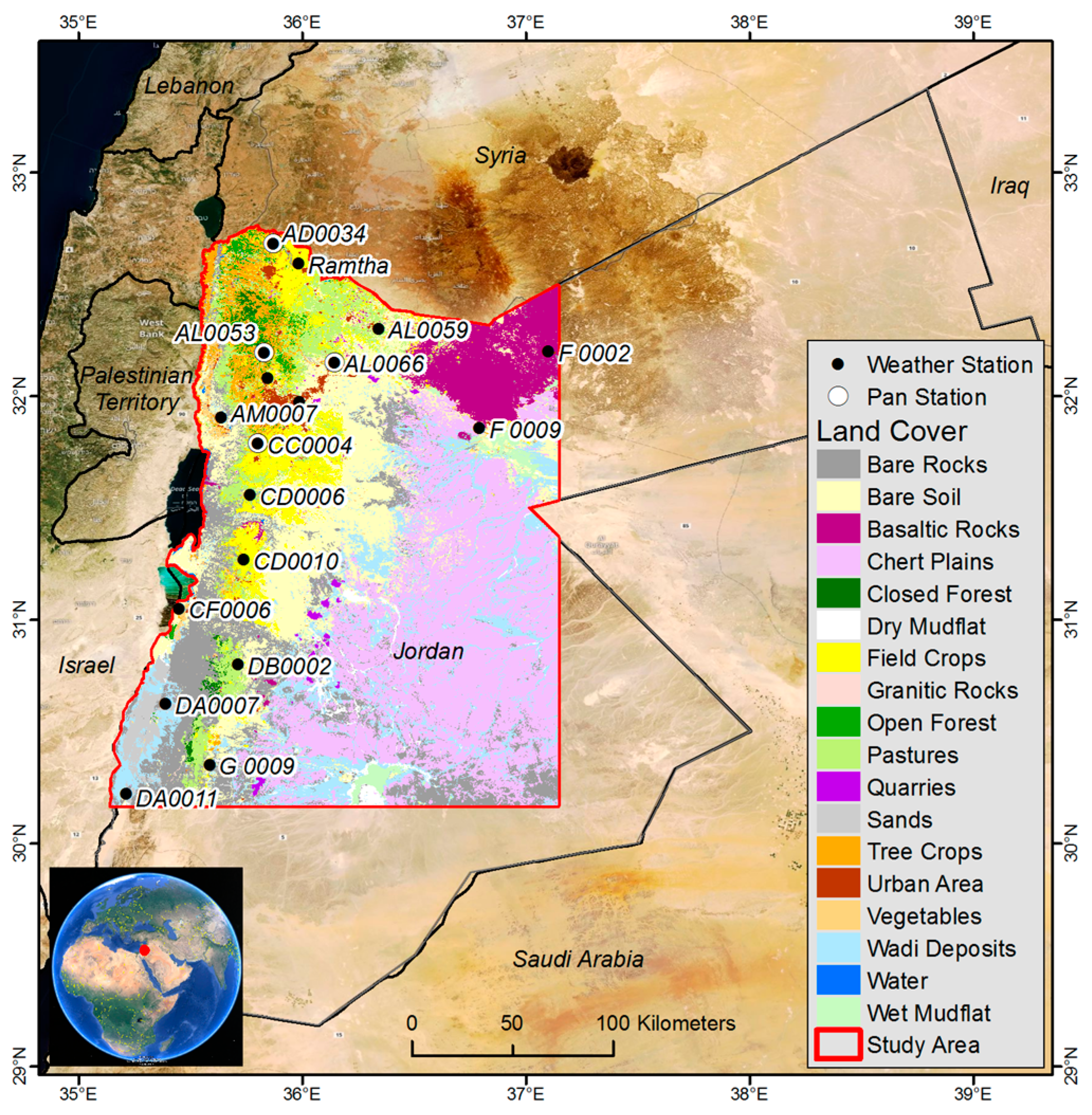
2.1. Study Area and Data

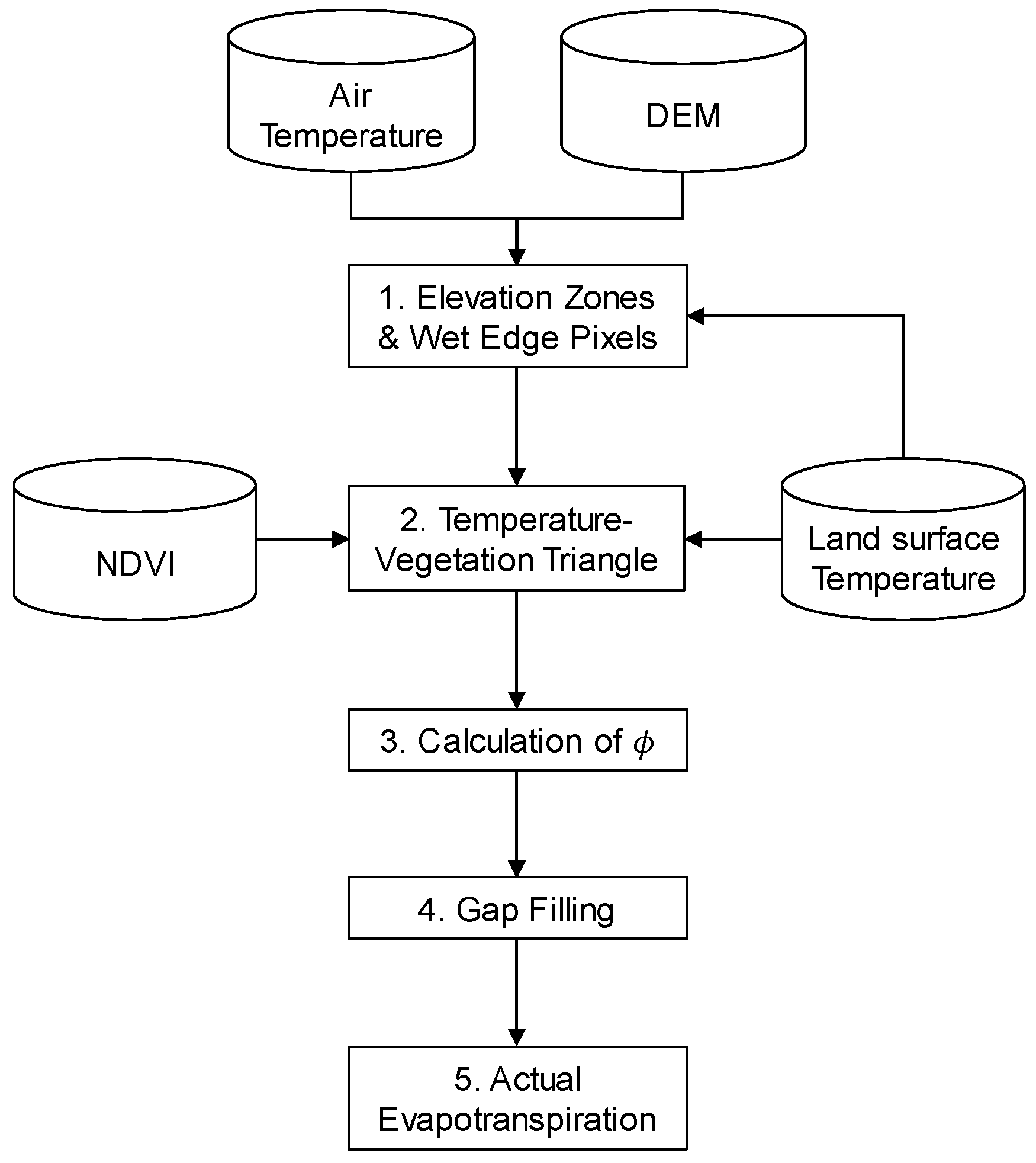
Located between 29°11′N and 33°22′N latitude and between 34°19′E and 39°18′E longitude, Jordan is one of the driest countries in the world (Figure 1). Over 80% of the country is arid or semi-arid, receiving less than 100 mm rainfall annually. The country shows significant north-south and west-east rainfall gradients, with the majority of rainfall occurring between October and April [26,27]. Rainfall has declined at an average rate of 0.4 mm/year over the past 40 years [28]. Annual pan evaporation varies between 2000 and 4500 mm, greatly exceeding annual rainfall across the country. Elevation in Jordan varies from −415 m at the shoreline of the Dead Sea to 1719 m in the southern highlands, which has a clear effect on T_s. As shown in Figure 2, T_s in areas below 200 m is generally higher than areas above 900 m on a typical summer day. Such a difference appears to reflect the terrain effects on T_s as both elevation zones have similar NDVI distributions, indicating that Jordan presents a relevant study region to investigate terrain effects on temperature-vegetation triangle methods. Our study region in the northwestern region of Jordan has an area of 42,056 km² and contains 99% of the country’s vegetated land surface as well as ~95% of the country’s population.

Jordan is ranked as one of the world’s water-poorest countries, where annual water per capita is only 145 m³ [29] in contrast to the international water poverty threshold of 1000 m³. It is considered among the most vulnerable nations in the world in terms of freshwater supply [30]. Agriculture is the dominant sector of water consumption. Rainfed agriculture is limited to the western highlands, where olive trees and cereals are cultivated, and to parts of the steppe region, where barley is cultivated [29]. Irrigated agriculture in Jordan has expanded rapidly in recent decades. From 1994 to 2013, the total area of agricultural land increased by 19%, but irrigated areas of tree crops and vegetables increased by 101% and 56%, respectively [31]. The expansion of irrigated agriculture, particularly of irrigated olive orchards, has posed unprecedented challenges to the water sustainability and security in Jordan. Due to intensified transboundary competition for surface water resources in the Jordan River basin, groundwater exploitation has played a critical role in Jordan’s water security. Consequently, in Jordan’s major basins, the water table is declining at an average rate of 1 m/year and by 2030 the average aquifer saturated thickness could decline by 30%−40% [32]. Despite a number of national and international initiatives aimed at evaluating water security and supply in Jordan, the magnitude and extent of groundwater use in the country, especially in the highlands where irrigated agriculture is thriving, remain highly uncertain. In the absence of on-the-ground data sources, deduction of agricultural water use through satellite-based AET estimates can provide important insight into water management issues for the country.

In this study, we use 23 sets of satellite images for 2009 from the MODIS daily 1-km T_s product (MOD11A1) and the 16-day 250-m NDVI product (MOD13Q1). The images were downloaded, mosaicked and re-projected using the MRTWeb tool from the Land Processes Distributed Active Archive Center of the United States Geological Survey. Within each of the 8-day NDVI windows, the 1-km daily T_s product with the least cloud cover was selected to represent the average land surface temperature over the 8 days. Both NDVI images and DEM were resampled to 1-km spatial resolution of the T_s images. Jordan’s Ministry of Water and Irrigation and local research collaborators provided a 90-m DEM and daily weather records (air temperature, precipitation, wind speed, humidity, radiation, and pan evaporation) from 14 stations. Potential evapotranspiration (PET) was calculated using the FAO Penman-Monteith equation [33]. Meteorological data for the PET calculation were extracted from the 0.5°-resolution Climate Forecast System Reanalysis data in the Global Weather Database managed by the Texas A&M University.

2.2. Methodology

Figure 3 presents the framework of the proposed TAVE method. It discretizes a DEM into a number of overlapping elevation zones and constructs the temperature-vegetation space for each elevation zone. The estimates of the parameter φ are first generated for individual elevation zones and then aggregated. The fitted dry edge is extended to a hypothetical “fully-vegetated” pixel. The wet edge reflects vegetation conditions and migrates with elevation zones. After clouded pixels are filled, φ values are converted into evaporative fraction estimates to generate AET rates. Compared to existing terrain correction methods, TAVE does not employ external information beyond the satellite images to modify the T_s or elevation data. Compared to traditional triangle algorithms, TAVE improves the determinations of wet and dry edges to address the prevailing water stress in semi-arid environments. The detailed procedures of TAVE are described below.

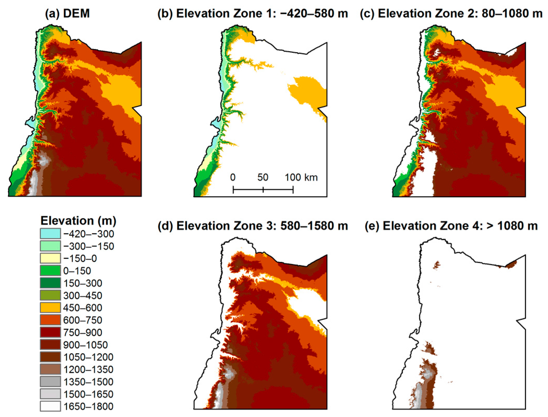
2.2.1. Elevation Zones and Wet Edge Pixels

The 1-km DEM of the study area is divided into a number of overlapping elevation zones (Figure 4). The width of an elevation zone is set based on the assumption that the terrain effect on T_s is negligible within this range of elevation variation. Adjacent elevation zones overlap by a defined value. The decisions regarding the zone width and overlap takes into consideration the resolution of satellite images to ensure the inclusion of a sufficient number of pixels for the triangle algorithm. In this study, with coarse-resolution MODIS data (250-m and 1000-m products), the width and overlap of elevation zones are set to 1000 m and 500 m, respectively. Smaller values would be applicable for images with higher resolution. Sensitivity of these parameters is discussed in Section 4.3. In contrast to the use of non-overlapping elevation zones where a single pixel is analyzed only once, overlapping elevation zones allow most of the pixels to be analyzed multiple times.

In the determination of the wet edge, on each specific date, TAVE identifies only one wet pixel over the domain, but multiple wet edges corresponded to different elevation zones. First, before the establishment of elevation zones, the pixel with the lowest T_s value over the entire domain is identified as the wet pixel. We visually examined the locations of wet pixels using a combination of Google Earth, Landsat images and land use maps. With the size of 1 km², each wet pixel proved to be a mixture of different land cover categories dominated by open water surface, irrigated cropland or forest. Second, after the elevation zones are established, for the elevation zone that contains the wet edge pixel, the wet edge is set to the T_s value of the wet pixel. For other elevation zones, the wet edge is estimated using a linear temperature lapse rate derived from annual average air temperature observations across weather stations at different elevations. In this study, a lapse rate of 0.55 °C/100 m was estimated using records from 14 stations spanning elevations from 13 m to 962 m (Figure S1 in Supplementary Information).

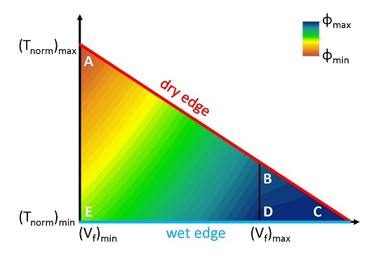
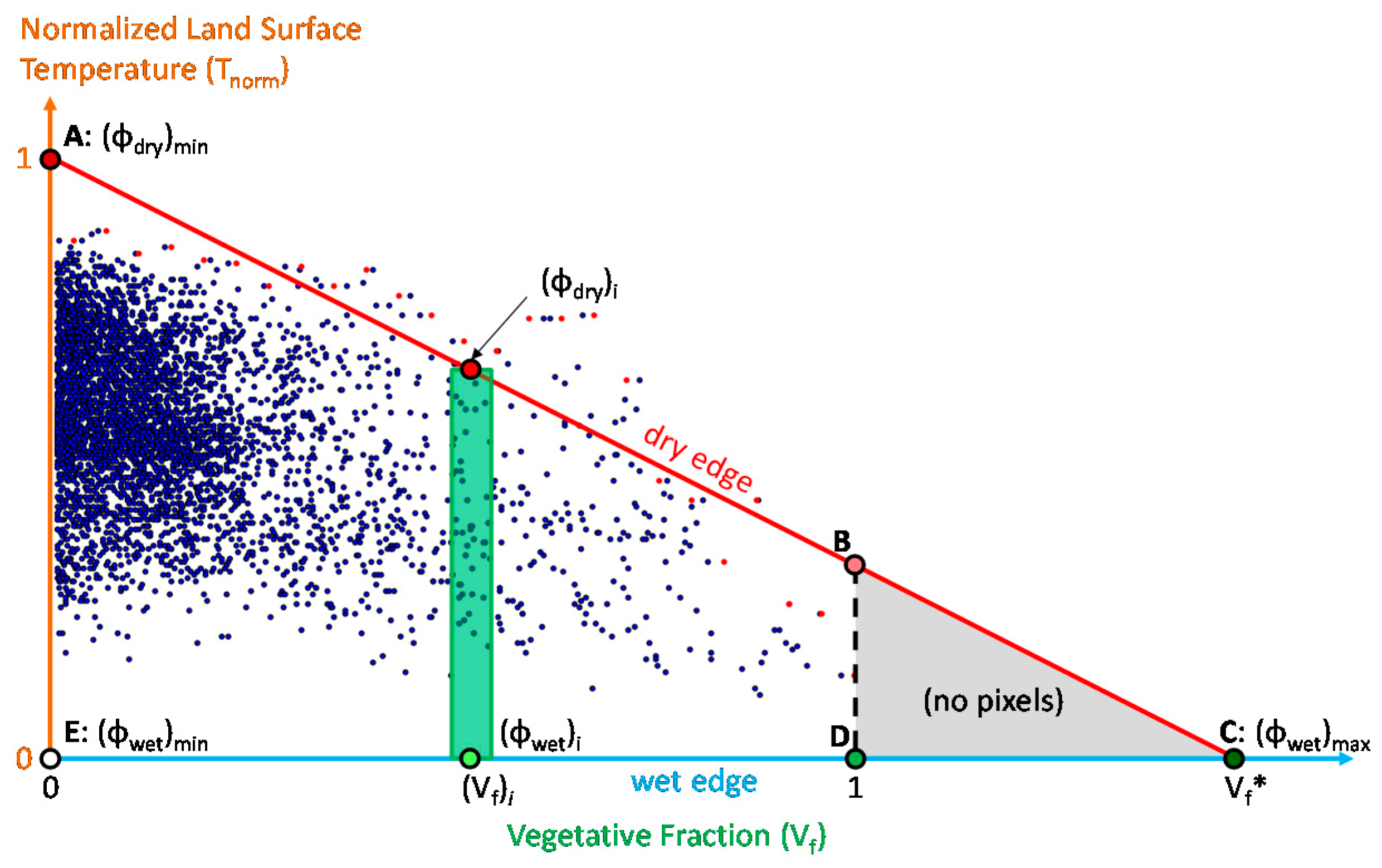
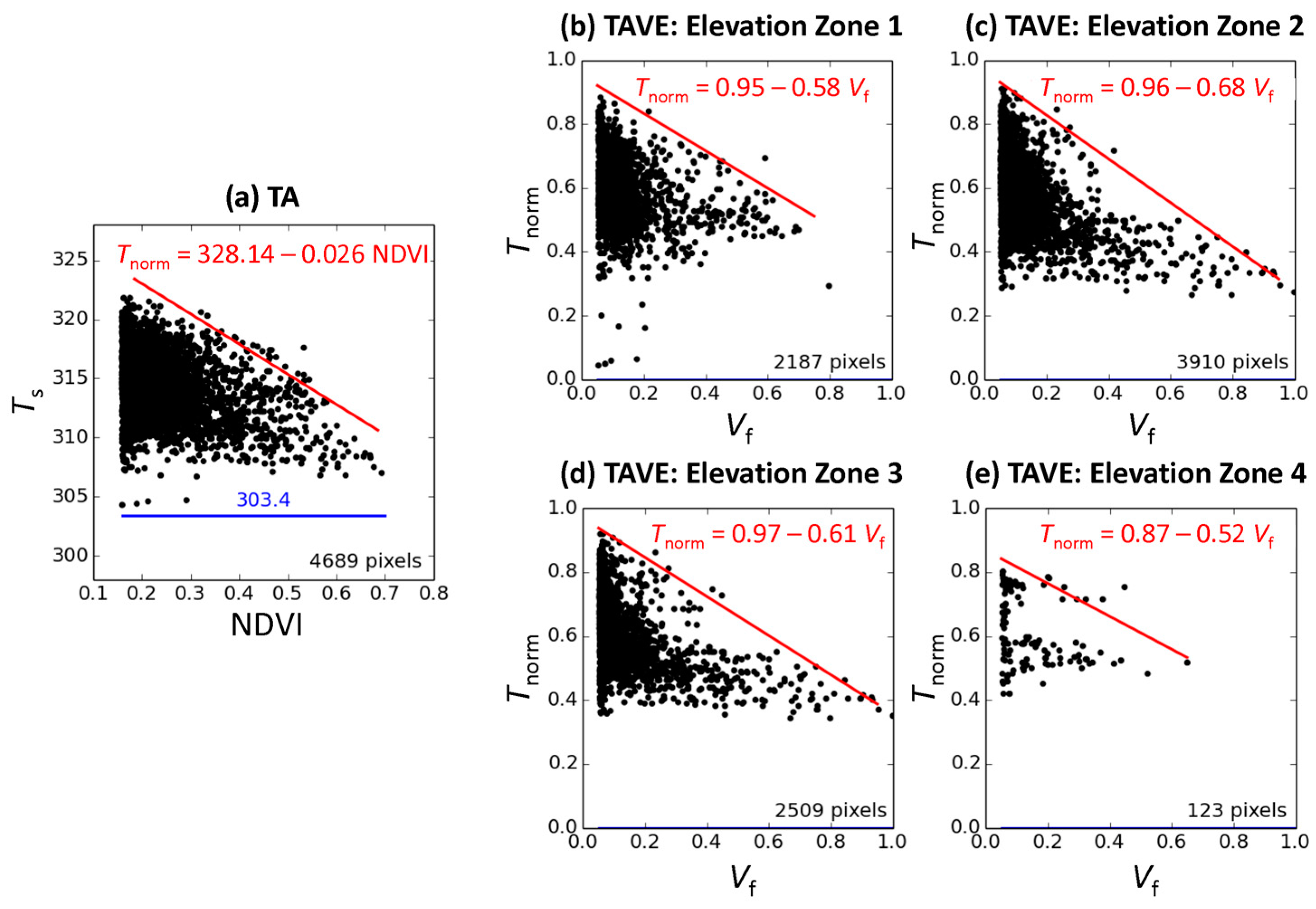
2.2.2. Establishment of the Temperature-Vegetation Triangle

For each elevation zone, a subset of NDVI and T_s images is extracted to establish the temperature-vegetation space (Figure 5). For the T_s layer, cloudy pixels (T_s = 0) are masked out and then T_s is converted into normalized land surface temperature, T_norm:

$$T_{\mathrm{norm}}=\frac{T_{\mathrm{s}}-T_{\mathrm{wet}}}{{(T_{\mathrm{s}})}_{\max }-T_{\mathrm{wet}}}$$

(1)

where (T_s)_max is the maximum T_s value across the domain and T_wet is the temperature of the wet edge as determined in 2.2.1. Therefore, the wet edge is always located at T_norm = 0 in the temperature-vegetation space. Although converting absolute T_s values to relative T_s values does not affect the values of the combined-effect parameter φ, the use of normalized T_s ensures that the triangles are presented within the same y-axis range. This facilitates the comparison of triangles from different seasons across a wide range of temperature. The use of normalized T_s has been also reported in other studies [18,34,35].

The NDVI layer is converted into vegetative fraction, V_f, using the formula proposed by Carlson and Ripley [36]:

$$V_{\mathrm{f}}={\left(\frac{\mathrm{NDVI}-{\mathrm{NDVI}}_{\min }}{{\mathrm{NDVI}}_{\max }-{\mathrm{NDVI}}_{\min }}\right)}^2$$

(2)

where NDVI_max and NDVI_min are the maximum and minimum NDVI values across the domain, respectively. The maximum and minimum NDVI values are examined using Google Earth, Landsat images and land use maps to ensure that they physically correspond to bare ground and fully vegetated surfaces, respectively. From a temporal perspective, the observed minimum NDVI value across different growth stages may not fully represent the vegetation condition of no physiological activity. However, from a spatial perspective, if the domain contains a wide range of vegetation and land cover conditions, the bare ground can be easily identified using an NDVI threshold. This is particularly so for semi-arid regions such as Jordan, where vegetation cover accounts for only 9% of the total area. In this study, non-vegetated pixels are excluded using a simple threshold: NDVI < 0.16. This threshold was determined by comparing non-vegetated pixels in NDVI images to land-use maps of Jordan of 2007 and 2014. Although there are some uncertainties with the physical conditions of maximum NDVI values (e.g., the discrimination of irrigated olive trees from forests) in a specific image, we have verified the characterization of non-vegetated areas based on land use maps and the derived NDVI threshold.

The dry edge is determined through linear regression (Figure 5). All of the pixels are grouped into a number of vegetation bins of equal size. The size of each bin is set to 0.05 of V_f (Equation (2)) for the case of MODIS images in this study. A smaller bin size could be applicable for satellite images with higher resolution. The algorithm identifies the maximum T_norm value of each bin and then performs a linear fit through all of the maximum T_norm values. The fitted maximum T_norm values across all of the bins constitute the dry edge.

2.2.3. Calculation of the Parameter φ

The dry edge is extended to intersect the wet edge and completes a triangle in the temperature-vegetation space (Figure 5). The intersection of the wet and dry edges indicates a hypothetical pixel that has a sufficiently-dense vegetation cover (V_f = V_f * > 1) that is able to fully satisfy the maximum value of the parameter φ. Along both the wet and dry edges, the value of φ varies linearly with V_f. The value of φ on the dry edge, (φ_dry)_i, uniformly increases from 0 at V_f = 0 to φ_max at V_f = V_f *, where φ_max = 1.26. The value of 1.26 is derived from the original Priestley-Taylor equation, arising empirically when evaporation approaches the available energy under equilibrium wet surface conditions. The 1.26 value has been found to correspond to the upper bound of derived φ values across different NDVI values and commonly used as the wet edge in other studies employing triangle algorithms [10,14]. A Soil-Vegetation-Atmosphere-Transfer (SVAT) model was aptly suggested for TA applications by Carlson [16,18] to determine variation in the combined-effect parameter φ along the wet edge. However, this was not done here for lack of data that included leaf area index, soil wilting point and field capacity, crop height, and stomata resistance. In the TAVE triangle for each elevation zone, the wet edge is the horizontal axis representing the lowest T_norm value (i.e., T_norm = 0) for the full range of NDVI values at that temperature. It is also the wet boundary of pixels because no pixel is cooler than the wet edge. The value of φ on the wet edge, (φ_wet)_i, uniformly increases from (φ_wet)_min = 0.5 φ_max at V_f = 0 to (φ_wet)_max = 1.0 φ_max at V_f = 1. In this study, the ratio of (φ_wet)_min to φ_max as 0.5 was selected based on the best fit to the data. It was estimated as the ratio of the domain-averaged NDVI value (0.13) to the updated NDVI average (0.26) after the NDVI threshold was applied to exclude pixels of bare ground. The intersection of the T_norm and V_f axes does not represent a pixel only containing wet soil, but rather a pixel with the lowest observed T_norm value.

It is assumed that soil moisture availability varies linearly between the dry and wet edges within a certain NDVI range. Therefore, the value of the parameter φ for a pixel i can be estimated based on the location of this pixel, [(T_norm)_i, (V_f)_i], in the temperature-vegetation space:

$${\varphi }_i=\left[1-{\left(T_{\mathrm{norm}}\right)}_i\right]\left[{\left({\varphi }_{\mathrm{wet}}\right)}_i-{\left({\varphi }_{\mathrm{dry}}\right)}_i\right]+{\left({\varphi }_{\mathrm{dry}}\right)}_i$$

(3)

where (φ_wet)_i and (φ_dry)_i are the φ values on the wet and dry edges at (V_f)_i. After all of the overlapping elevation zones are processed, for each pixel, the mean of all of its zone-level estimates is calculated as the final estimate of φ.

2.2.4. Gap Filling

This method uses MODIS datasets of different time scales: the daily T_s images (MOD11A1) and the 16-day NDVI images (MOD13Q1). The NDVI images are temporal composite products, representing maximum NDVI values derived from daily raw observations over a 16-day period, and the number of cloudy pixels is very low in these composite images. Daily T_s images normally contain more pixels masked by clouds. If the pixel is cloudy on both T_s and NDVI images, it is excluded from the analysis. If the pixel is cloudy in the daily T_s image but cloud-free in the 8-day composite NDVI image, a two-step gap filling procedure is performed to estimate their φ values. For each cloudy pixel, the method assesses its V_f value and identifies all of the cloud-free pixels in the same vegetation bin. For example, if a pixel is cloudy in the T_s image and has a V_f value of 0.32, the φ value of this pixel is the average φ value of all of the cloud-free pixels with V_f values between 0.30 and 0.35, given the size of the vegetation bin is 0.05. In the extreme case when a vegetation bin contains only cloudy pixels, this vegetation bin is excluded if the number of cloudy pixels is large, or the image-wide average φ value is used if the number of cloudy pixels is small. However, neither extreme case was observed in this study, as we selected the daily T_s image with the least cloud cover for each 8-day time window. Over a total of 23 T_s images of 2009, the cloud cover varies from 0% to 26% with an average of 6% (Figure S2 in Supplementary Information). The percentage of cloudy vegetated pixels that need to be treated is even lower, so the gap filling has negligible effect on the ET estimates.

This spatial gap filling approach is also adopted to address the unique land cover pattern of northwestern Jordan (Figure 1). The vegetation-bare ground boundaries are very clear. The majority of areas with medium- or high-density vegetation cover tend to exist as continuous patches within certain elevation ranges, e.g., irrigated agriculture regions in the valley below −100 m or forest reserves in the highlands above 600 m (see Figure 1 and Figure 4a). This situation provides acceptable conditions to fill isolated cloudy pixels with the average value of adjacent pixels with similar vegetation conditions. However, the spatial gap filling is less effective for areas with low vegetation cover, since these areas span a wide range of land surface and atmospheric conditions where the AET rates could range from minimum to maximum.

2.2.5. Calculations of AET

The instantaneous evaporative fraction (EF), defined as the ratio of latent heat flux to available energy [13], is calculated based on the composite-effect parameter φ:

$$\mathrm{EF}=\varphi \left[\frac{\mathsf{\Delta }}{\mathsf{\Delta }+\mathsf{\gamma }}\right]$$

(4)

where ∆ is the slope of saturated vapor pressure versus air temperature (kPa K⁻¹), and γ is the psychrometric constant (kPa K⁻¹). A digital elevation model and air temperature from the climate reanalysis data are used to calculate ∆ and γ. The sensitivity of ∆/(∆ + γ) to the variation of temperature is small [10,14].

Recent studies suggest that the midday EF is very close to the average daytime EF [37,38]. As the overpass time of the Terra Satellite is 10:30 AM local time and reasonably close to the range of midday times, we assume the calculated instantaneous EF remains constant throughout the daytime. This assumption has been widely adopted in other MODIS-based evapotranspiration studies [39,40]. Therefore, the daily AET (mm/day) is estimated as:

$$\mathrm{AET}=\left[\mathrm{EF}\left(R_{\mathrm{n}}-G\right)\right]/\lambda$$

(5)

where R_n and G are respectively net radiation and soil heat flux during daytime (MJ m⁻² day⁻¹) and λ is the latent heat of vaporization (MJ kg⁻¹). Following the procedure developed by Allen [33], R_n is estimated using air temperatures, wind speed, solar radiation, albedo, elevation, and geographic coordinates. Weather variables are obtained from the climate reanalysis data. Albedo is calculated based on MODIS reflectance data (MOD09GA), using the method proposed by Tang et al. [41]. G is estimated as a fraction of R_n based on typical values [42]. The TAVE-derived daily AET estimate is assumed to be constant within the 8-day period of MODIS data, and the 16-day cumulative AET estimates are then summed to generate monthly, seasonal and annual estimates.

3. Results

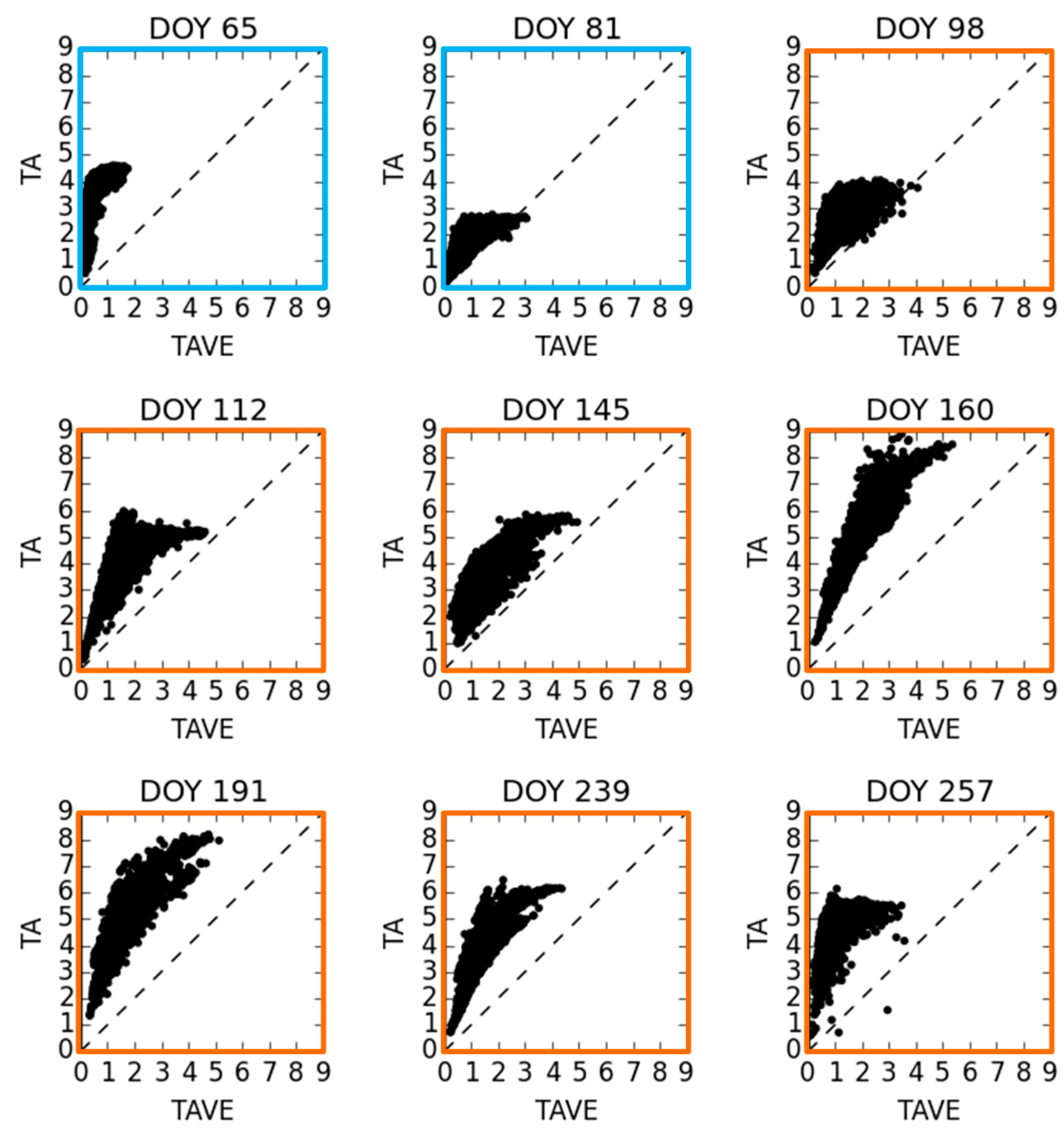
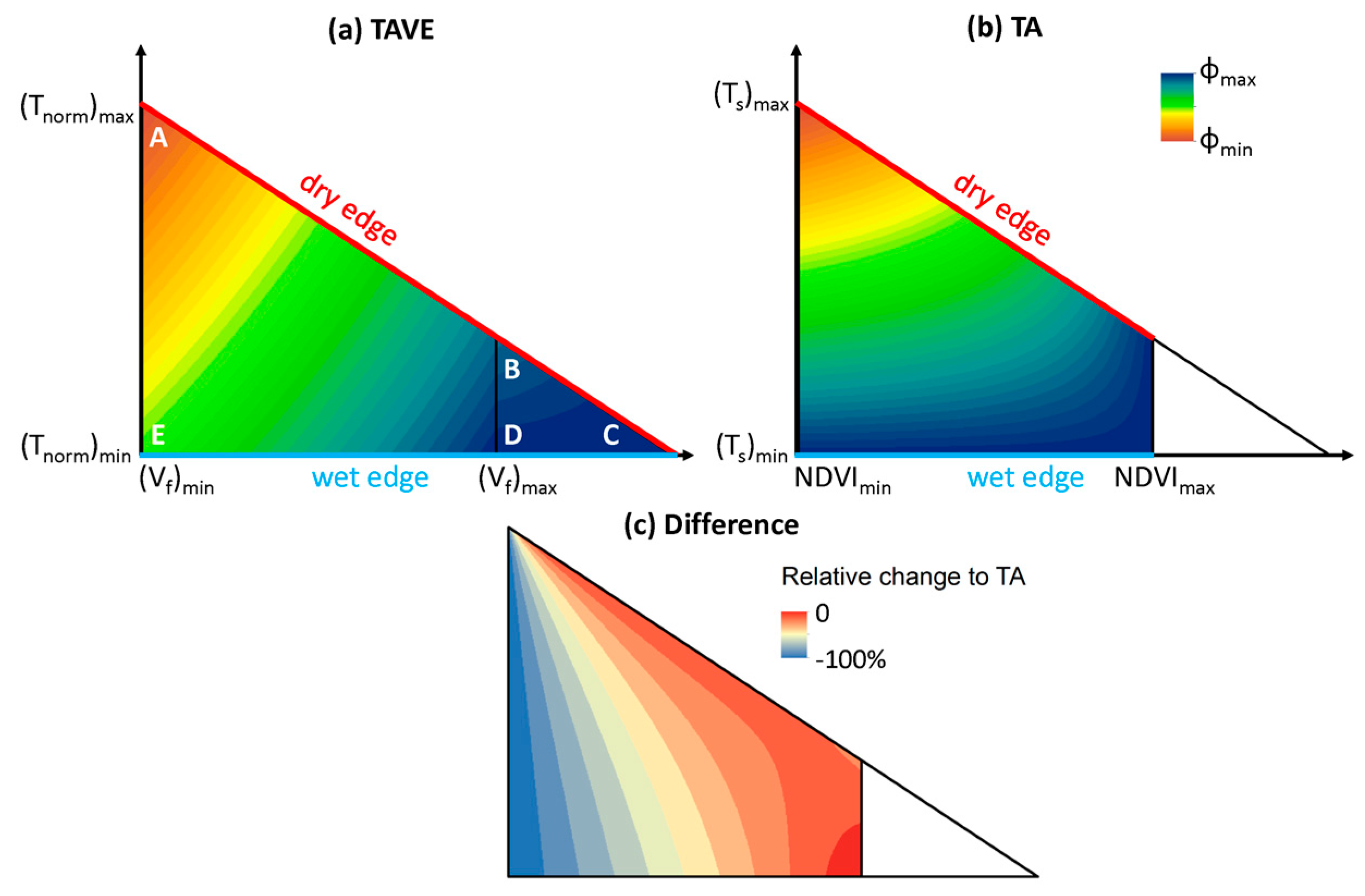
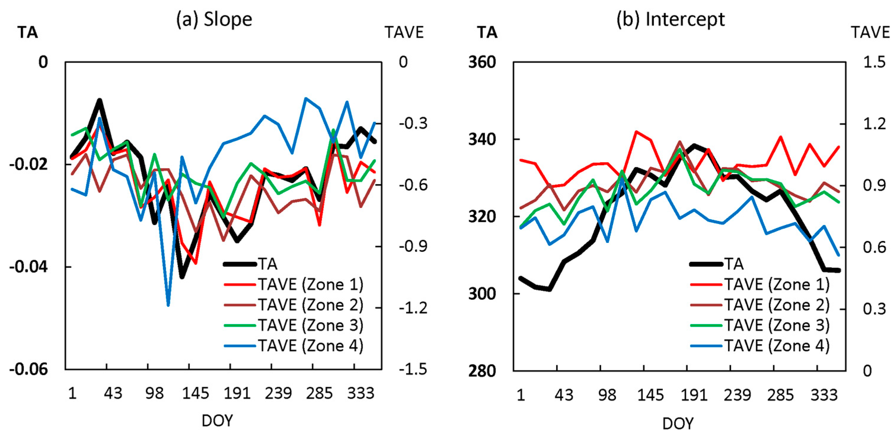
3.1. Comparison of TAVE with the Original Single Triangle Method

Figure 6 compares the temperature-vegetation triangles generated by TAVE and a traditional triangle method [10]. In contrast to the single triangle of TA, TAVE establishes four triangles based on four overlapping elevation zones. Each elevation zone contains a sufficient number of vegetated pixels (>2000) for identifying a triangle, except for the highest elevation zone (above 1080 m) where only 123 vegetated pixels are available. As most of the pixels are included in two elevation zones and are therefore included twice in the total pixel count, the four triangles of TAVE show a total of 8729 pixels, compared to the 4689 pixels shown in the triangle of TA. Although the dry edges are well identified in all triangles, TA and TAVE differ on the locations of wet edges. The wet edge of TA is based on the T_s of the pixel with the highest NDVI value; in the triangles of TAVE, the wet edge is always consistent with a horizontal axis at T_norm = 0.

Figure 7 shows the performance of TAVE compared with TA on nine days in 2009, which are selected to reflect a range of representative sets of wet and dry season conditions. The estimates by TA are consistently higher than that by TAVE, especially during the dry season when the available energy is abundant. Indeed, the TA-derived AET rates occasionally approach PET rates in Jordan, which conflicts with the reality of Jordan’s semi-arid environment where rainfall is considerably lower than PET.

Figure 8 presents the variation of slope and intercept of the dry edge for 2009. Overall, TAVE and TA show similarity in the seasonal pattern of the dry edge. The dry season (April–September) appears to have lower slope and higher intercept than the wet season (October–March), as the maximum T_s values in the dry season are generally higher than those in the wet season. This pattern is less recognizable for Elevation Zone 4 (blue line), as this zone contains a much smaller number of pixels.

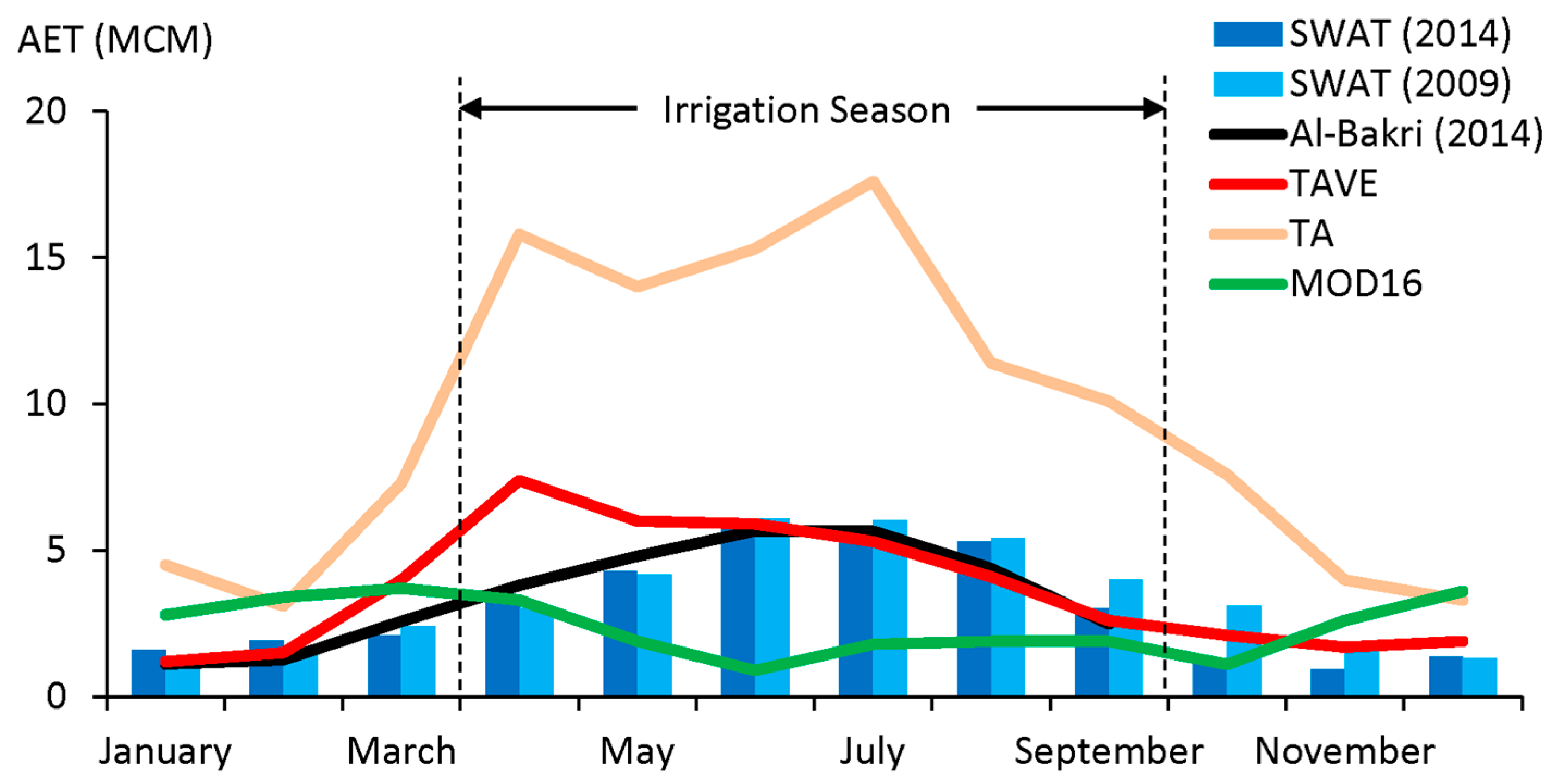
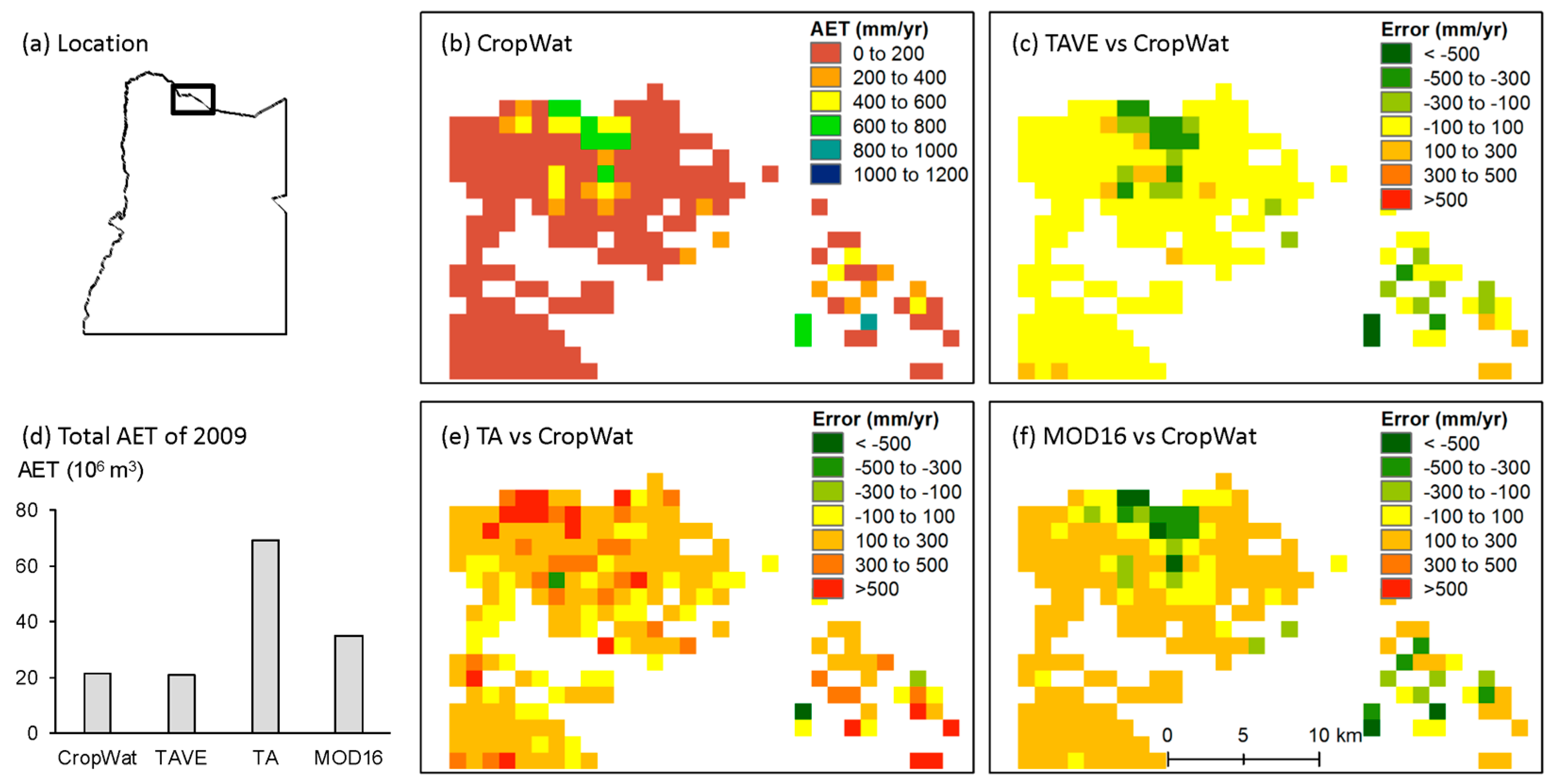
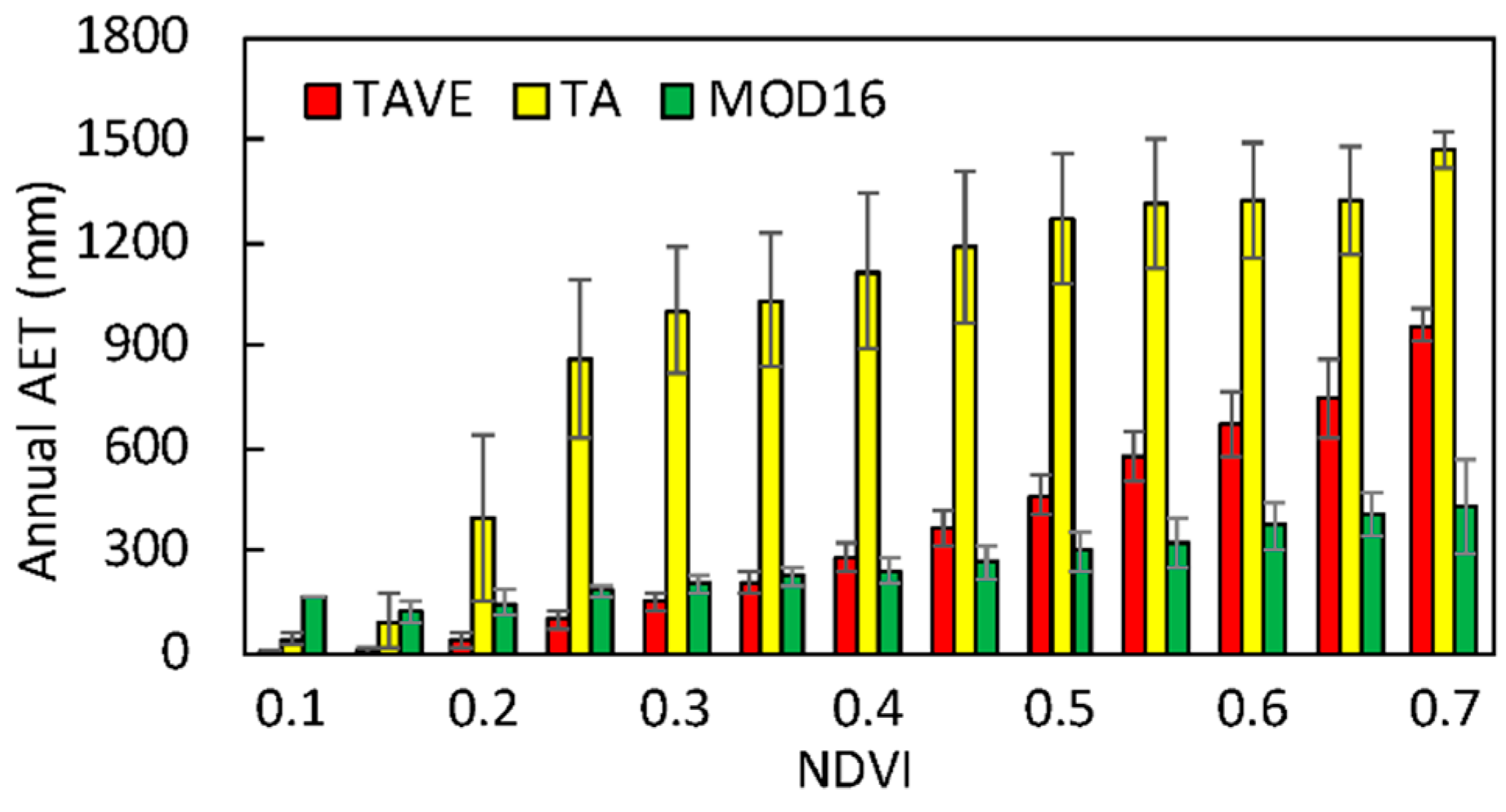
3.2. Comparison of AET Estimates in Agricultural Irrigated Lands

Validation of satellite-derived AET estimates at the regional scale is not possible directly, as the spatial footprint of ground AET instruments (on the order of 100 m²) is not comparable to the pixel size of MODIS images (1 km²) [19]. This is particularly so for sparsely-populated countries with limited in situ monitoring such as Jordan, where the lack of aperture scintillometer or eddy flux tower systems has resulted in a scarcity of AET observations over the heterogeneous landscape. Here we compare satellite-derived AET estimates with the results of the single crop coefficient model using CropWat [33]. The main inputs to CropWat include weather records from a ground station (AL0059), shown in Figure 1, a 30-m land use map derived from Landsat images, soil data [43], and the growth stages and coefficients of five major crop species (i.e., olive trees, eggplant, citrus, lettuce and tomato) [33]. The crop coefficient-derived AET estimates are used as a proxy for ground truth as this method has been successfully validated in many agricultural areas in arid or semi-arid regions [44,45]. As the single crop coefficient method was primarily developed for irrigation planning, the comparison focuses on the Yarmouk River Basin in Jordan (Figure 9a), an area with extensive irrigated croplands during the dry season. In addition, we expand the comparison to the MODIS global evapotranspiration product (MOD16) [46,47]. MOD16 is the first regular 1-km land surface evapotranspiration data set for global vegetated land areas and has been widely used around the world.

Across the entire Yarmouk River Basin in Jordan, the TAVE-derived AET estimate over irrigated lands during the irrigation season (April-September) is 31.3 million m³ (MCM). This is comparable to the estimated agricultural water use (26.8 MCM) reported in a local study [48] employing Landsat imagery and the single crop coefficient model (Figure 9). We attribute the difference primarily to two factors. First, the comparison involves different years, i.e., 2009 in this study versus 2014 in Al-Bakri [48]. Climate reanalysis data show that 2009 was wetter (+185 mm for total precipitation) and cooler (−1.3 °C for average temperature) than 2014. The likelihood that the climatic conditions in 2009 favors higher AET is borne out by hydrologic simulation of the Yarmouk River Basin. Simulation using the Soil Water Assessment Tool (SWAT) [49] indicated that the total AET during the irrigation season in 2009 was 28.7 MCM, 4.4% higher than SWAT results in 2014 (27.4 MCM). The reliability of SWAT modeling was verified using observed stream flow at the Adasiya station. Second, the comparison is affected by the disparity in spatial resolution, i.e., MODIS 1-km pixels in this study and the Landsat 30-m pixels in Al-Bakri [48]. Due to the small size of irrigated farms in this region, many 1-km pixels contain extensive non-irrigated surface. The TAVE-derived AET estimate at each pixel therefore can reflect a combined effect of irrigation-enhanced AET and rainfall-controlled AET. Such mixed land-use within pixels is less pronounced in the 30-m pixels of Landsat. Rainfall data with high spatial resolution (on the order of 1~10 km²) may facilitate the separation of rainfall-controlled AET, but the quantification and unmixing of sub-pixel variations in MODIS imagery remain a challenge in remote sensing [50,51,52].

We also compare TAVE to TA and MOD-16 derived estimates. In contrast to TAVE’s estimate of 31.3 MCM, the TA-derived estimate of 84.2 MCM greatly exceeds the 2009 reference evapotranspiration of 50.0 MCM. The MOD16-derived estimate of 11.7 MCM shows substantial underestimation and does not reflected irrigation-enhanced AET. Comparing 2009 monthly values, we see that irrigation-season estimates in particular based on TAVE appear to be more reasonable for this semi-arid environment (Figure 9).

Figure 10 and Figure 11 present results for the eastern portion of the Yarmouk River Basin, where over 90% of the agricultural lands are irrigated. Figure 10 shows the comparison of four types of AET estimates by TAVE, TA, MOD16, and CropWat on 9 June 2009. This date was selected as it was cloud free and near the peak-NDVI date for several major crops in Jordan during the irrigation season. The selection of images was introduced above in the section Study Area and Data. In terms of the total AET (Figure 9b), TAVE is comparable to CropWat (+38%), in contrast to the substantial overestimation by TA (+474%) and underestimation by MOD16 (−94%). The overestimation by TA is larger than 1 mm/day across all pixels (Figure 9d); the underestimation by MOD16 is as much as 0.93 mm/day, particularly evident in areas with intensive irrigation (Figure 9c). The sound performance of TAVE is further demonstrated at the annual level (Figure 11). The CropWat-derived total AET is well matched by TAVE (−3%), in contrast to the substantial overestimation by TA (+234%) and underestimation by MOD16 (−50%). In terms of spatial pattern, the intensively-irrigated areas remain overestimated by TA and underestimated by MOD16, but both of them tend to yield underestimations for sparsely-vegetated areas. Overall, the results indicate that TAVE works well in agricultural irrigated lands in a semi-arid region, where TA and MOD16 greatly overestimate and underestimate AET, respectively.

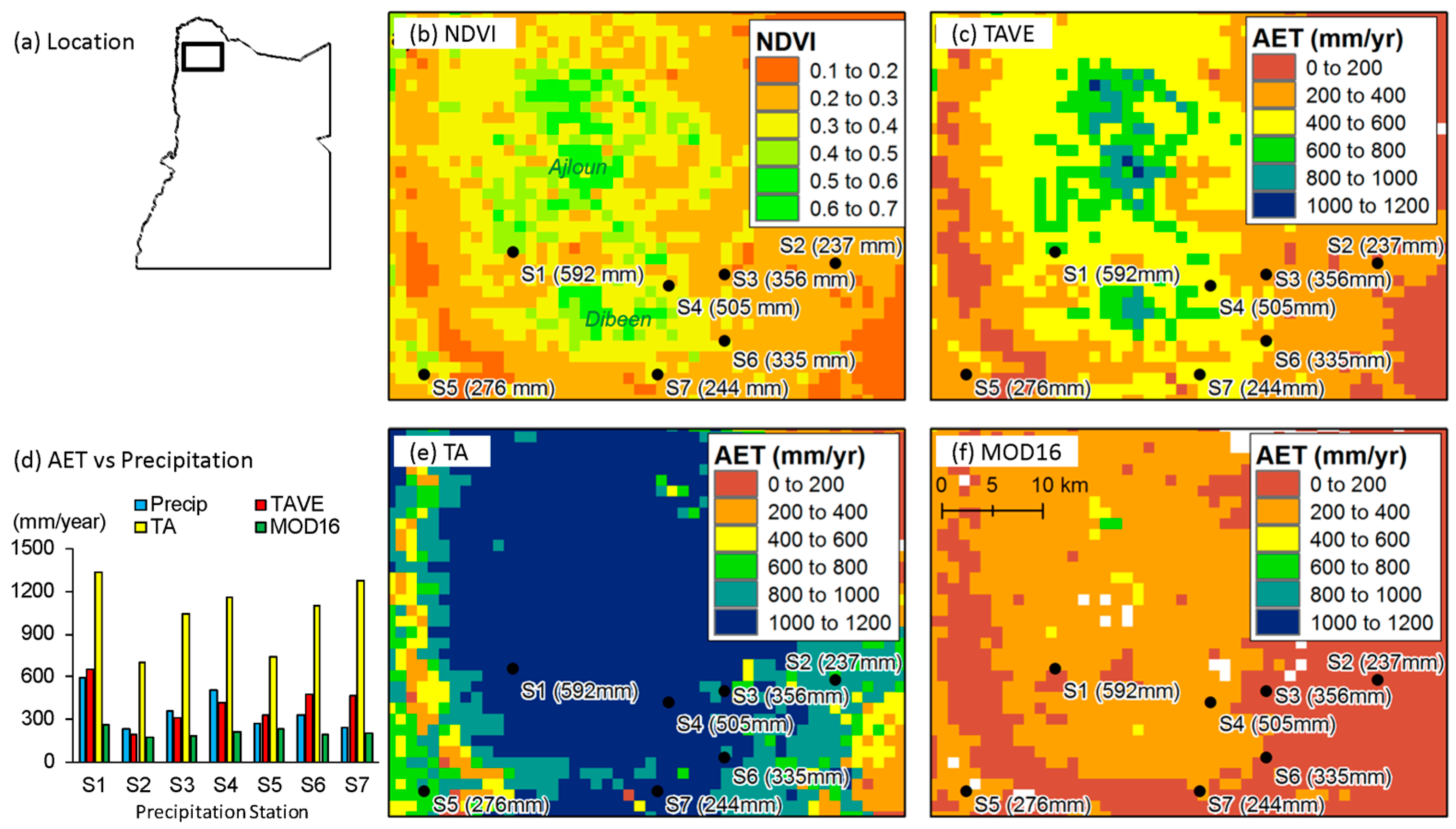
3.3. Comparison of AET Estimates in Naturally Vegetated Areas

Evapotranspiration in arid and semi-arid regions is a water-limited process. In areas with deep water tables and without irrigation, the annual precipitation was shown to approach the annual AET rate [53]. Here we compare different AET estimates to the precipitation in the Ajloun and Dibeen Forest Reserves in the study area (Figure 12). These forests show high NDVI values and irrigation is negligible in this mountainous region with the water table deeper than 110 m [54]. Rainfall observations are available in this region at seven weather stations that cover a variety of elevation and vegetation conditions. Across different weather stations (Figure 12b), TAVE’s estimates are more comparable with annual precipitation. The mean deviations of TAVE, TA and MOD16 results with observed precipitation are 44 mm, 684 mm and −153 mm, respectively, and the root mean square errors (RMSE) are 0.31 mm day⁻¹, 1.94 mm day⁻¹ and 0.52 mm day⁻¹, respectively. This result is comparable to the range of RMSE reported for triangle methods [35] and MOD16 [55]. In terms of the spatial distribution of AET, TAVE captures the boundary of forests and reflects the variation in annual precipitation. TA results substantially exceed the maximum observed annual precipitation, and MOD16 results show little variation despite the observed precipitation heterogeneity.

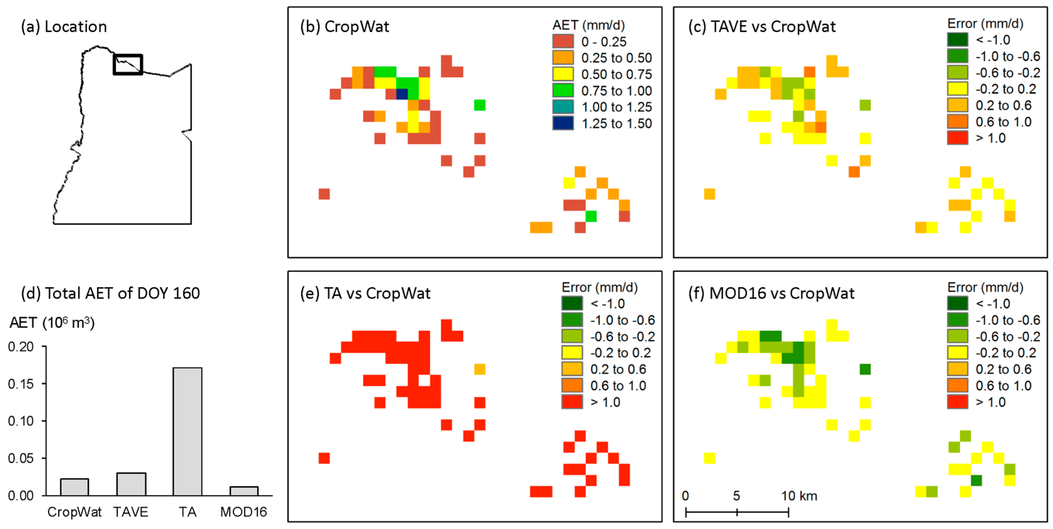
3.4. Comparison of AET Estimates over the Study Area

We compare the annual AET estimates by TAVE, TA and MOD16 across different NDVI intervals over the entire study area (Figure 13). Across the NDVI range of 0.25−0.70, all of the methods are able to address the positive control of vegetation cover on AET rates with comparable spatial patterns, and TAVE appears to occupy a middle ground between TA and MOD16. The estimates given by TAVE are 35%−88% lower than that given by TA. Compared with MOD16, TAVE appears to underestimate AET for low NDVI values and overestimate for high NDVI values. As summarized by Hu et al. [55], MOD16 performs best at sites located in forest regions or in a temperate and fully humid climate; it tends to underestimate AET over poorly vegetated surface in a semi-arid or arid climate such as the Mediterranean, Sahel, Southern Africa regions, and the Central Great Plains of the United States. Additional comparisons between TA, TAVE and MOD16 are presented in the Supplementary Information (Figures S3 to S6). Overall, our results indicate that TAVE is an effective method to correct the overestimation by TA and the underestimation by MOD16.

4. Discussion

4.1. Determining Wet and Dry Edges in Semi-Arid Environments

The identification of the dry and wet edges has been a major challenge to triangle methods and resulted in many misconceptions since they were introduced [16]. This problem is analogous to the identification of wet and dry pixels in many end-member methods including some widely-used energy balance models such as SEBAL and METRICS, despite the contrast in the degrees of complexity of these methods. A fundamental question confronted by many studies is whether the dry and wet edges are identifiable in the image. In other words, can we actually observe the three points that constitute the temperature-vegetation triangle, especially the intersection point of the wet and dry edges? We argue that this critical point is often not observable in coarse-resolution images of semi-arid environments, due to the combined effects of water stress and landscape heterogeneity. Rather than search for an ideal pixel to validate this point, we estimate the position of this pixel in the temperature-vegetation space, taking into consideration terrain effects, to control the distribution of the parameter φ within the triangle. In particular, the determination of dry and wet edges in TAVE differs from that in traditional triangle methods in two respects: i) the positions of edges and ii) the distributions of φ along the edges.

In terms of edge positions, the wet edge has received more attention than the dry edge. Various methods have been proposed to locate the wet edge based on various indicators, such as the minimum T_s at the maximum NDVI [11], the mean or linear regression of minimum T_s values across different NDVI intervals [56], average temperature of inland waterbodies [6], or air temperature [57].

In this study, TAVE determines the minimum T_s in the domain and establishes a variable wet edge that migrates with elevation zones, leading to an implicit but effective consideration of terrain effects. The dry edge is determined by fitting the maximum temperature across vegetation intervals and then both wet and dry edges are extended to form the triangle. An important feature of the TAVE-derived triangle is that the triangle consists of two regions: a trapezoid region that contains the pixels observed in the images and a triangle region that represents moisture conditions not observable with current image resolution; the two regions are shown as ABDE and BCD in Figure 5, respectively.

In terms of the distributions of φ along the edges, TAVE is significantly different from traditional triangle methods. The common practice for the wet edge is to set a constant maximum $\varphi$ on the edge, so the maximum EF is independent of vegetation conditions. As for the dry edge, different distributions of φ have been discussed (see for example, Long et al. [17]). The existing methods assume that the upper bound of the highest vegetation interval have either the strongest AET capacity (e.g., φ = φ_max and EF = 1) or the weakest AET capacity (e.g., φ = φ_min and EF = 0). Both assumptions are questionable in semi-arid environments. On one hand, semi-arid regions have low fractional vegetation cover compared to humid regions. For example, LAI and NDVI values of the study area are below 1.5 and 0.7, respectively. Pixels with the maximum NDVI values in the image do not necessarily have the highest EF due to the prevailing water stress, particularly in the dry season. Only under the conditions with fully sufficient moisture supply such as an open water surface or well-irrigated crops does EF approach one. Assuming fully vegetated areas are associated with EF = 1 will lead to the overestimation of AET. On the other hand, EF in areas with dense vegetation cover cannot be zero. Even in semi-arid environments, zero evapotranspiration rarely occurs for dense vegetation cover due to root zone soil water uptake [13]. Therefore, the maximum land surface temperature over a certain vegetation interval does not promise a zero EF. EF is never absolutely zero even in the middle of a desert, and evaporation over wet bare soil can be higher than ET of dense vegetation.

TAVE is the first triangle method that introduces a scheme of dual variable edges. On both wet and dry edges, φ linearly increases from a specified minimum value to 1 as vegetation increases from the threshold to the theoretical saturated vegetation condition. To maintain the φ gradient between the two boundary conditions across vegetation intervals, φ increases more quickly on the wet edge and reaches its maximum value at the maximum observed vegetation fraction (V_f = 1). Both dry and wet edges are extended to a hypothetical position. The pixel is assumed to have a sufficient vegetation fraction and the ability to satisfy φ_max. Such a configuration leads to significant change in the distribution of φ across the triangle. Compared with the traditional triangle, the TAVE-derived triangle has reduced φ values across the triangle as shown in Figure 14, particularly over low vegetation cover, and shows an enhanced linkage of vegetation condition to φ values.

The observed difference between the results of TAVE and TA in this study is primarily caused by the configuration of the wet edge (i.e., the location of the edge and the variation of φ values along the wet edge) and the unique environment conditions of Jordan. On the one hand, in general, TAVE will generate lower φ values than those generated by TA. As shown in the conceptual comparison in Figure 14, TAVE-derived φ values can be up to 100% lower than TA-derived φ values, depending on the location of pixel in the triangle. This is particularly so for pixels with low vegetation cover across the whole temperature range. This is also observed in with real data of Jordan as shown in Figure 13, where pixels with NDVI < 0.3 exhibit the greatest difference between TAVE and TA. On the other hand, these sparsely-vegetated pixels cover the majority of the study domain. The average NDVI value for the entire domain is only 0.13, and 0.26 even after bare ground is excluded. These sparsely-vegetated pixels occupy the areas in the triangle, where TAVE and TA differ most. As a result, the TA-vs-TAVE difference is highlighted in our typical case of semi-arid environment.

TAVE is consistent with other triangle methods in the reliance on φ. Although this parameter accounts for aerodynamic and surface resistance, vapor pressure gradient, and soil moisture availability in an integrative manner, it does not explicitly address the variations of canopy structure, infrastructure height and wind speed that could affect the distribution of aerodynamic resistance. However, through establishing overlapping elevation zones to better characterize dry and wet edges, TAVE highlights the importance of taking into consideration the variation of elevations when applying triangle methods. The findings of this study suggest that efforts focusing on other surface or atmospheric factors might further improve the performance of triangle methods over a heterogeneous landscape.

4.2. Temperature Control Versus Vegetation Control

The traditional triangle algorithms, as well as the widely-used surface energy models, rely heavily on daytime T_s. The reliability of satellite-derived daily T_s products is known to be impacted by errors associated with view angle, heavy dust aerosols in semi-arid environments, uncertainties in surface emissivity, and cloud cover, especially at regional scales [58,59,60,61]. Small errors in T_s may result in significant uncertainties in AET estimates by surface energy models; for example, a 2-K difference of T_s could result in up to a 15% change in AET estimates [4]. Indeed, complex energy balance models are not recommended for estimating AET when dealing with large scales. For triangle methods where T_s is scaled between maximum and minimum, the absolute errors of T_s are less influential, but they remain a source of uncertainty in AET estimates. This is particularly so when the spatial variation of instantaneous T_s may not reflect the spatial variation of latent heat flux at the daily scale in water-limited environments [42,62].

Figure 15 compares T_s to NDVI on 9 June (DOY 160) and 25 June (DOY 176), 2009, over the northern region of the study area. The images of DOY 176 show that higher NDVI values are associated with lower T_s values, suggesting stronger evapotranspiration. The pattern of NDVI shows little variation between DOY 160 and DOY 176 across different landscapes from forests to rainfed and irrigated agricultural lands (Figure 14b), which is consistent with stable T_s values observed in most areas (B1 to B4 in Figure 15a). This indicates that evapotranspiration is an essential control on T_s in these areas. However, some irrigated agricultural lands see a 10-15 K decrease of T_s on DOY 160 (B5 and B6 in Figure 15a). This is unlikely to be caused by reduced evapotranspiration as temporary NDVI changes between DOY 160 and DOY 176 are negligible in both B5 and B6. A possible reason for such a contradiction is that T_s can be significantly influenced by synoptic weather conditions and has large variations. Based on the nearest weather station (AL0059, shown in Figure 1), there was no rainfall between DOY 160 and DOY 176, but the daily average wind speed on DOY 159 was 112% higher that of DOY 175, indicating the potential of a strong wind effect on T_s in 24 hours. This example leads to concern about whether T_s should play a dominant role in generating satellite-based AET estimates in semi-arid regions where evapotranspiration may not be closely linked with T_s variations due to weather dynamics. In addition, using 8-day composite T_s instead of daily T_s may improve the availability of cloud-free pixels, but the exclusion of cooler cloudy days could result in the overestimation of T_s at the average overpass time.

In contrast to the uncertainties associated with T_s, remotely-sensed vegetation indices address the relatively slow surface processes of vegetation dynamics that can be reasonably assumed to be stable over several days. More importantly, for semi-arid environments like Jordan, the actual evapotranspiration process is largely water limited instead of energy limited. Water stress is prevailing throughout the year except for some well-irrigated regions. The healthy status of vegetation directly reflects the availability of soil moisture and is less sensitive to other environmental factors. The dependence on vegetation indices contributes to the success of several satellite-based evapotranspiration models including the globally-applied MOD16 product [62]. The proposed TAVE aims to enhance the role of vegetation within the framework of triangle algorithms through adjusting the triangle’s dry and wet edges based on terrain and vegetation variations, but preserves the control of T_s on the φ values of pixels with similar vegetation conditions.

4.3. Sensitivity Analysis

Here we examine the sensitivity of TAVE-estimated EF to five parameters: width of elevation zones, overlap of elevation zones, number of vegetation bins, NDVI threshold, and temperature lapse rate. Results of sensitivity analyses are included in the Supplementary Information (Figure S7 in Supplementary Information). The width and overlap of elevations zones control the discretization of the DEM. Results indicate that EF estimates increase by 12% when the zone width increases from 500 m to 1000 m. The overlap of elevation zones has negligible influence on the EF estimates with < 2% change when this parameter is increased from 100 m to 500 m. The number of vegetation bins and NDVI threshold control the influence of NDVI images in the triangle analysis. AET increases 17% when the number of vegetation bins is increased from 5 to 20. The NDVI threshold is applied to exclude pixels of bare soil. The response of EF estimates to NDVI threshold variations shows an increase between 0.13 and 0.15. This is mainly caused by the exclusion of sparsely vegetated areas in the eastern part of the study area that is adjacent to the desert region. Such areas have negligible potential for agricultural development and are thus not as significant in terms of water resources management. The lapse rate controls the establishment of wet edges. A lower lapse rate results in higher temperature of wet edges and thus higher ET estimates. Over the domain, the average EF under a lapse rate of 0.02 °C/100 m is 11.5% higher than that under a lapse rate of 0.75 °C/100 m. Overall, the EF estimates by TAVE are generally insensitive to the above parameters, slightly decreasing with the lapse rate and increasing with other parameter values.

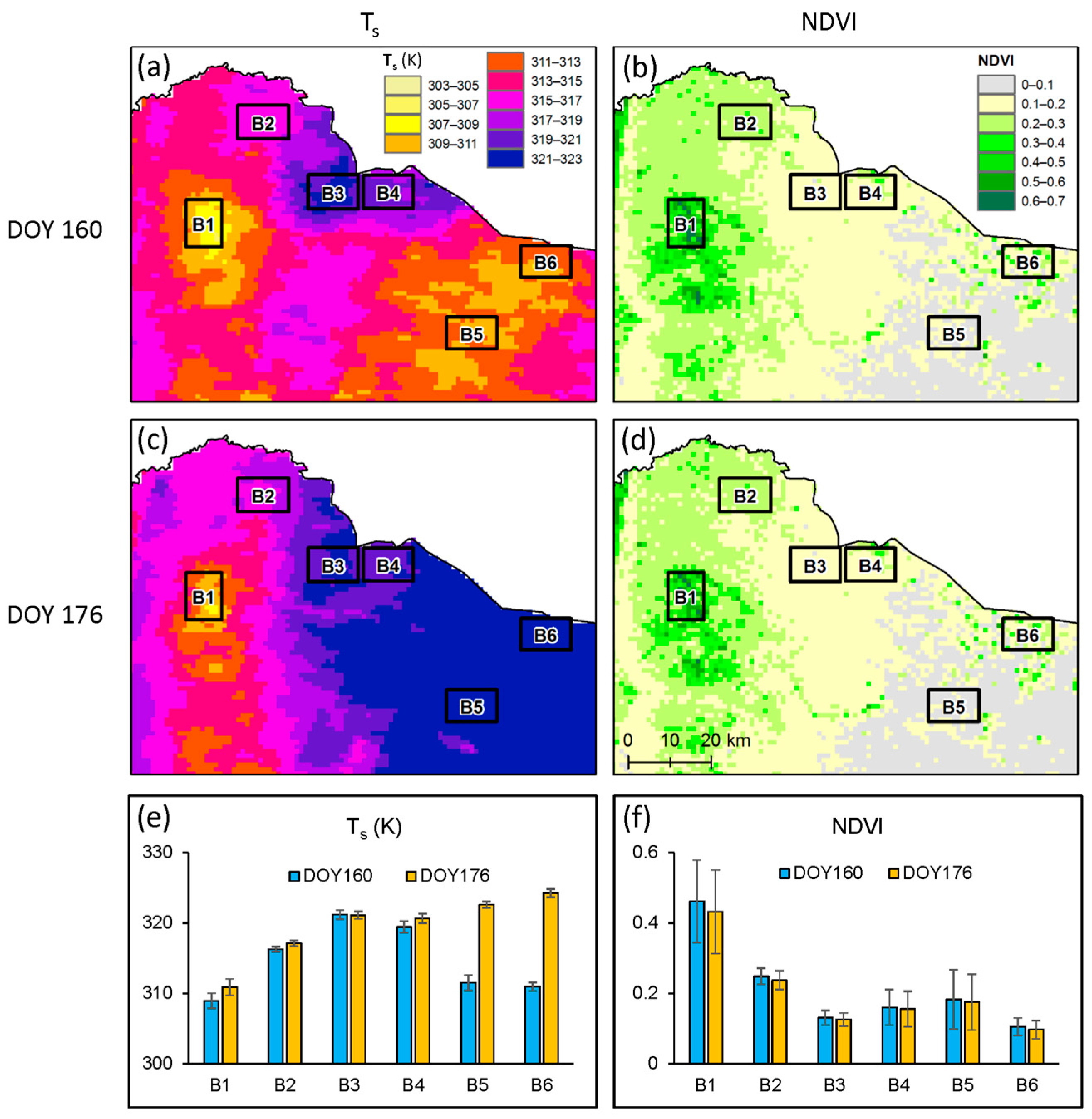
4.4. The Effect of Image Spatial Resolution

The proposed TAVE method can be applied to other satellite images of land surface temperature and vegetation. In this study, we used MODIS data instead of Landsat data mainly for two related reasons: (i) the small revisit cycle of two days, which improves the possibility of obtaining a cloud-free T_s image in each time window and enhances the temporal resolution of ET variation; and (ii) the large view swath of 2330 km, which covers the study area with one scene and thus circumvents the efforts of image mosaic and registration. These advantages come with the sacrifice of spatial resolution. Although the TAVE method is able to identify ET hotspots such as irrigated croplands and forests across the study area, the 1-km resolution of MODIS data is insufficient to capture local hotspots in a heterogeneous landscape. For example, in the Yarmouk River Basin (Figure 10 and Figure 11) where smaller farm plots are prevalent, the spatial pattern of ET estimates can be better characterized if 100-m Landsat thermal images were employed. High spatial resolution will also influence the determination of dry and wet edges through identifying the pixels associated with lowest and highest T_s values. For example, the identification of pixels of impervious surfaces from airborne images have a strong control on the dry edge [12]. A recent study [63] shows that Landsat-derived AET estimates can explain 91% of the variability in the observed AET, in contrast to 59% by MODIS-based estimates.

Triangle methods show strong dependency on spatial resolution and generally perform better across large areas (on the order of 10⁴ km²) compared to small areas (on the order of 10² km²) [4]. The decision between MODIS and Landsat appears to be a tradeoff between spatial resolution and temporal resolution, depending on the research objective. If the goal is to determine regional water consumption during a specific growth stage or over a short time period, MODIS inputs would provide finer information on the temporal dynamics. If the goal is to identify the water consumption of specific crop species or small-sized farms, Landsat would be more useful. An improvement in the general spatial and temporal resolution of satellite instruments would allow for a better understanding of the biophysical properties encapsulated within the temperature-vegetation triangles, as well as more detailed triangle-based studies of the land-atmosphere energy fluxes [35].

5. Conclusions

We propose a new Triangle Algorithm with Variable Edges (TAVE) to improve satellite-based regional actual evapotranspiration estimates in semi-arid regions. This method is an improvement over traditional triangle algorithms based on three unique features: (i) the discretization of the domain as overlapping elevation zones; ii) a variable wet edge that migrates with elevation zones; and iii) variable evaporative fraction values along both wet and dry edges. TAVE can effectively address the combined influence of terrain and water stress on AET estimates in semi-arid environments. We have applied this method with MODIS data to one of the most water-poor countries in the world—Jordan. Results from TAVE are compared with a traditional triangle method and a widely-used global ET product (MOD16), using the single coefficient model and annual precipitation as proxies for ground truth. In irrigated agricultural lands, TAVE matched the results of the single coefficient model (−3%), in contrast to the substantial overestimation by TA (+234%) and underestimation by MOD16 (−50%). In forested (non-irrigated, water consuming) regions, TA and MOD16 produced AET average deviations 15.5 times and −3.5 times of those based on TAVE. Results suggest that TAVE is an effective method to generate AET estimates in semi-arid environments.

As TAVE has a simple structure and low data requirements, it provides an efficient solution to the increasing need of evapotranspiration estimation in data-scarce developing countries. TAVE can be applied to other semi-arid environments and only requires remotely sensed land surface temperatures and the well-known measure of green vegetation, NDVI, plus a DEM. In contrast to previous attempts in which the domain-wide lump T_s and NDVI data could mask the underlying signal and efficacy of triangle methods, TAVE represents a semi-distributed scheme to discretize the altitude effects on triangle methods and provides a template to address the heterogeneity of other physical factors. This work demonstrates the improved performance of triangle methods when the domain is disaggregated into more homogeneous areas in the vertical dimension. TAVE can be expanded to take into consideration the horizontal dimension, e.g., using land use or soil factors to further discretize the domain. In addition to the spatial dimensions, temporal patterns could also be better addressed based on the framework of TAVE through: (i) clustering images into different groups based on their atmospheric conditions and adjusting wet/dry edges at the group level; and (ii) developing 3-D triangles to characterize the trajectory of wet/dry edges at the seasonal or annual levels. Finally, we note that this study constitutes an essential step towards the satellite-based quantification of irrigation water use and effective water resources management in Jordan as well as other semi-arid regions with high freshwater vulnerability.

References

1. Chehbouni, A.; Escadafal, R.; Duchemin, B.; Boulet, G.; Simonneaux, V.; Dedieu, G.; Mougenot, B.; Khabba, S.; Kharrou, H.; Maisongrande, P.; et al. An integrated modelling and remote sensing approach for hydrological study in arid and semi-arid regions: The sudmed programme. Int. J. Remote Sens. 2008, 29, 5161–5181. [Google Scholar] [CrossRef] [Green Version]
2. Chirouze, J.; Boulet, G.; Jarlan, L.; Fieuzal, R.; Rodriguez, J.C.; Ezzahar, J.; Er-Raki, S.; Bigeard, G.; Merlin, O.; Garatuza-Payan, J.; et al. Intercomparison of four remote-sensing-based energy balance methods to retrieve surface evapotranspiration and water stress of irrigated fields in semi-arid climate. Hydrol. Earth Syst. Sci. 2014, 18, 1165–1188. [Google Scholar] [CrossRef] [Green Version]
3. Loheide, S.P.; Gorelick, S.M. A local-scale, high-resolution evapotranspiration mapping algorithm (ETMA) with hydroecological applications at riparian meadow restoration sites. Remote Sens. Environ. 2005, 98, 182–200. [Google Scholar] [CrossRef]
4. Long, D.; Singh, V.P.; Li, Z.L. How sensitive is Sebal to changes in input variables, domain size and satellite sensor? J. Geophys. Res. 2011. [Google Scholar] [CrossRef]
5. Moffett, K.B.; Nardin, W.; Silvestri, S.; Wang, C.; Temmerman, S. Multiple stable states and catastrophic shifts in coastal wetlands: Progress, challenges, and opportunities in validating theory using remote sensing and other methods. Remote Sens. 2015, 7, 10184–10226. [Google Scholar] [CrossRef]
6. Jiang, L.; Islam, S.; Guo, W.; Singh Jutla, A.; Senarath, S.U.S.; Ramsay, B.H.; Eltahir, E. A satellite-based daily actual evapotranspiration estimation algorithm over South Florida. Glob. Planet. Chang. 2009, 67, 62–77. [Google Scholar] [CrossRef]
7. Batra, N.; Islam, S.; Venturini, V.; Bisht, G.; Jiang, L. Estimation and comparison of evapotranspiration from MODIS and AVHRR sensors for clear sky days over the southern great plains. Remote Sens. Environ. 2006, 103, 1–15. [Google Scholar] [CrossRef]
8. Jiang, L.; Islam, S. Estimation of surface evaporation map over southern great plains using remote sensing data. Water Resour. Res. 2001, 37, 329–340. [Google Scholar] [CrossRef]
9. Jiang, L.; Islam, S. An intercomparison of regional latent heat flux estimation using remote sensing data. Int. J. Remote Sens. 2003, 24, 2221–2236. [Google Scholar] [CrossRef]
10. Jiang, L.; Islam, S. A methodology for estimation of surface evapotranspiration over large areas using remote sensing observations. Geophys. Res. Lett. 1999, 26, 2773–2776. [Google Scholar] [CrossRef]
11. De Tomás, A.; Nieto, H.; Guzinski, R.; Salas, J.; Sandholt, I.; Berliner, P. Validation and scale dependencies of the triangle method for the evaporative fraction estimation over heterogeneous areas. Remote Sens. Environ. 2014, 152, 493–511. [Google Scholar] [CrossRef]
12. Li, Z.; Jia, L.; Lu, J. On uncertainties of the Priestley-Taylor/LST-FC feature space method to estimate evapotranspiration: Case study in an arid/semiarid region in northwest china. Remote Sens. 2014, 7, 447–466. [Google Scholar] [CrossRef]
13. Stisen, S.; Sandholt, I.; Nørgaard, A.; Fensholt, R.; Jensen, K.H. Combining the triangle method with thermal inertia to estimate regional evapotranspiration—Applied to MSG-SEVIRI data in the Senegal river basin. Remote Sens. Environ. 2008, 112, 1242–1255. [Google Scholar] [CrossRef]
14. Tang, R.; Li, Z.L.; Tang, B. An application of the TS–VI triangle method with enhanced edges determination for evapotranspiration estimation from modis data in arid and semi-arid regions: Implementation and validation. Remote Sens. Environ. 2010, 114, 540–551. [Google Scholar] [CrossRef]
15. Wang, W.; Huang, D.; Wang, X.G.; Liu, Y.R.; Zhou, F. Estimation of soil moisture using trapezoidal relationship between remotely sensed land surface temperature and vegetation index. Hydrol. Earth Syst. Sci. 2011, 15, 1699–1712. [Google Scholar] [CrossRef]
16. Carlson, T.N. Triangle models and misconceptions. Int. J. Remote Sens. Appl. 2013, 3, 155–158. [Google Scholar]
17. Long, D.; Singh, V.P.; Scanlon, B.R. Deriving theoretical boundaries to address scale dependencies of triangle models for evapotranspiration estimation. J. Geophys. Res. 2012. [Google Scholar] [CrossRef]
18. Carlson, T. An overview of the “triangle method” for estimating surface evapotranspiration and soil moisture from satellite imagery. Sensors 2007, 7, 1612–1629. [Google Scholar] [CrossRef]
19. Rasmussen, M.O.; Sørensen, M.K.; Wu, B.; Yan, N.; Qin, H.; Sandholt, I. Regional-scale estimation of evapotranspiration for the north China plain using MODIS data and the triangle-approach. Int. J. Appl. Earth Obs. Geoinf. 2014, 31, 143–153. [Google Scholar] [CrossRef]
20. Van Doninck, J.; Peters, J.; De Baets, B.; De Clercq, E.M.; Ducheyne, E.; Verhoest, N.E.C. Influence of topographic normalization on the vegetation index-surface temperature relationship. J. Appl. Remote Sens. 2012. [Google Scholar] [CrossRef]
21. Stroppiana, D. Seasonality of MODIS lst over southern Italy and correlation with land cover, topography and solar radiation. Eur. J. Remote Sens. 2014, 47, 133–152. [Google Scholar] [CrossRef]
22. Rahimzadeh-Bajgiran, P.; Omasa, K.; Shimizu, Y. Comparative evaluation of the vegetation dryness index (VDI), the temperature vegetation dryness index (TVDI) and the improved TVDI (ITVDI) for water stress detection in semi-arid regions of Iran. ISPRS J. Photogramm. Remote Sens. 2012, 68, 1–12. [Google Scholar] [CrossRef]
23. Hassan, Q.; Bourque, C.; Meng, F.R.; Cox, R. A wetness index using terrain-corrected surface temperature and normalized difference vegetation index derived from standard MODIS products: An evaluation of its use in a humid forest-dominated region of Eastern Canada. Sensors 2007, 7, 2028–2048. [Google Scholar] [CrossRef]
24. Zhao, X.; Liu, Y. Relative contribution of the topographic influence on the triangle approach for evapotranspiration estimation over mountainous areas. Adv. Meteorol. 2014, 2014, 1–16. [Google Scholar] [CrossRef]
25. Gorelick, S.M. Water Security in Jordan: A Key to the Future of the Middle East. Available online: https://www.brookings.edu/blog/planetpolicy/2015/01/16/water-security-in-jordan-a-key-to-the-future-of-the-middle-east/ (accessed on 27 August 2016).
26. Al-Bakri, J.T.; Suleiman, A.S. NDVI response to rainfall in different ecological zones in Jordan. Int. J. Remote Sens. 2004, 25, 3897–3912. [Google Scholar] [CrossRef]
27. Toernros, T.; Menzel, L. Addressing drought conditions under current and future climates in the Jordan River region. Hydrol. Earth Syst. Sci. 2014, 18, 305–318. [Google Scholar] [CrossRef]
28. Rahman, K.; Gorelick, S.M.; Dennedy-Frank, P.J.; Yoon, J.; Rajaratnam, B. Declining rainfall and regional variability changes in jordan. Water Resour. Res. 2015, 51, 3828–3835. [Google Scholar] [CrossRef]
29. Al-Bakri, J.T.; Salahat, M.; Suleiman, A.; Suifan, M.; Hamdan, M.R.; Khresat, S.; Kandakji, T. Impact of climate and land use changes on water and food security in jordan: Implications for transcending “the tragedy of the commons”. Sustainability 2013, 5, 724–748. [Google Scholar] [CrossRef]
30. Padowski, J.C.; Gorelick, S.M.; Thompson, B.H.; Rozelle, S.; Fendorf, S. Assessment of human–natural system characteristics influencing global freshwater supply vulnerability. Environ. Res. Lett. 2015. [Google Scholar] [CrossRef]
31. DOS. Crop Statistics of Jordan. Available online: http://www.dos.gov.jo/dos_home_e/main/ (accessed on 27 August 2016).
32. El-Naser, H.K. Water Security in the Middle East—“A Crisis on Top of A Crisis”. Available online: https://pangea.stanford.edu/researchgroups/jordan/jordan-minister-dr-hazim-el-naser-addresses-stanford-community-water-security-middle-east (accessed on 27 August 2016).
33. Allen, R.G.; Pereira, L.S.; Raes, D.; Smith, M. Crop. Evapotranspiration: Guidelines for Computing Crop Water Requirements; FAO: Rome, Italy, 1998. [Google Scholar]
34. Zhao, W.; Li, A. A downscaling method for improving the spatial resolution of AMSR-E derived soil moisture product based on MSG-SEVIRI data. Remote Sens. 2013, 5, 6790–6811. [Google Scholar] [CrossRef]
35. Petropoulos, G.; Carlson, T.N.; Wooster, M.J.; Islam, S. A review of TS/VI remote sensing based methods for the retrieval of land surface energy fluxes and soil surface moisture. Prog. Phys. Geogr. 2009, 33, 224–250. [Google Scholar] [CrossRef]
36. Carlson, T.N.; Ripley, D.A. On the relation between NDVI, fractional vegetation cover, and leaf area index. Remote Sens. Environ. 1997, 62, 241–252. [Google Scholar] [CrossRef]
37. Peng, J.; Borsche, M.; Liu, Y.; Loew, A. How representative are instantaneous evaporative fraction measurements of daytime fluxes? Hydrol. Earth Syst. Sci. 2013, 17, 3913–3919. [Google Scholar] [CrossRef]
38. Nichols, W.E.; Cuenca, R.H. Evaluation of the evaporative fraction for parameterization of the surface energy balance. Water Resour. Res. 1993, 29, 3681–3690. [Google Scholar] [CrossRef]
39. Kiptala, J.K.; Mohamed, Y.; Mul, M.L.; Van der Zaag, P. Mapping evapotranspiration trends using MODIS and Sebal model in a data scarce and heterogeneous landscape in eastern Africa. Water Res. Res. 2013, 49, 8495–8510. [Google Scholar] [CrossRef]
40. Rahimi, S.; Gholami Sefidkouhi, M.A.; Raeini-Sarjaz, M.; Valipour, M. Estimation of actual evapotranspiration by using MODIS images (a case study: Tajan catchment). Arch. Agron. Soil Sci. 2014, 61, 695–709. [Google Scholar] [CrossRef]
41. Tang, R.; Li, Z.L.; Chen, K.S.; Jia, Y.; Li, C.; Sun, X. Spatial-scale effect on the Sebal model for evapotranspiration estimation using remote sensing data. Agric. For. Meteorol. 2013, 174, 28–42. [Google Scholar] [CrossRef]
42. Waters, R.; Allen, R.; Tasumi, M.; Trezza, R.; Bastiaanssen, W. Surface Energy Balance Algorithms for Land (Idaho Implementation)—Advanced Training and Users Manual; Idaho Department of Water Resources: Boise, ID, USA, 2002. [Google Scholar]
43. Batjes, N.H.; Rawajfih, Z.; Al-Adamat, R. Soil Data Derived From Soter for Studies of Carbon Stocks and Change in Jordan (ver 1.0, Gefsoc Project); World Soil Information: Wageningen, The Netherlands, 2003; p. 34. [Google Scholar]
44. Ghamarnia, H.; Miri, E.; Ghobadei, M. Determination of water requirement, single and dual crop coefficients of black cumin (Nigella Sativa L.) in a semi-arid climate. Irrig. Sci. 2014, 32, 67–76. [Google Scholar] [CrossRef]
45. Hou, L.; Wenninger, J.; Shen, J.; Zhou, Y.; Bao, H.; Liu, H. Assessing crop coefficients for zea mays in the semi-arid Hailiutu river catchment, northwest China. Agric. Water Manag. 2014, 140, 37–47. [Google Scholar] [CrossRef]
46. Mu, Q.; Heinsch, F.A.; Zhao, M.; Running, S.W. Development of a global evapotranspiration algorithm based on MODIS and global meteorology data. Remote Sens. Environ. 2007, 111, 519–536. [Google Scholar] [CrossRef]
47. Mu, Q.; Zhao, M.; Running, S.W. Improvements to a MODIS global terrestrial evapotranspiration algorithm. Remote Sens. Environ. 2011, 115, 1781–1800. [Google Scholar] [CrossRef]
48. Al-Bakri, J.T. Mapping Irrigated Crops and Their Water Consumption in Yarmouk Basin; Jordan Ministry of Water and Irrigation: Amman, Arab, 2015.
49. Arnold, J.G.; Srinivasan, R.; Muttiah, R.S.; Williams, J.R. Large area hydrologic modeling and assessment—Part 1: Model development. J. Am. Water Resour. Assoc. 1998, 34, 73–89. [Google Scholar] [CrossRef]
50. Li, F.Q.; Kustas, W.P.; Anderson, M.C.; Prueger, J.H.; Scott, R.L. Effect of remote sensing spatial resolution on interpreting tower-based flux observations. Remote Sens. Environ. 2008, 112, 337–349. [Google Scholar] [CrossRef]
51. Ji, L.; Zhang, L.; Wylie, B. Analysis of dynamic thresholds for the normalized difference water index. Photogramm. Eng. Remote Sens. 2009, 75, 1307–1317. [Google Scholar] [CrossRef]
52. Lobell, D.B.; Asner, G.P. Cropland distributions from temporal unmixing of MODIS data. Remote Sens. Environ. 2004, 93, 412–422. [Google Scholar] [CrossRef]
53. Raz-Yaseef, N.; Yakir, D.; Schiller, G.; Cohen, S. Dynamics of evapotranspiration partitioning in a semi-arid forest as affected by temporal rainfall patterns. Agric. For. Meteorol. 2012, 157, 77–85. [Google Scholar] [CrossRef]
54. USGS. Groundwater-Level Trends and Forecasts, and Salinity Trends, in The Azraq, Dead Sea, Hammad, Jordan Side Valleys, Yarmouk, and Zarqa Groundwater Basins, Jordan; U.S. Geological Survey: Reston, VA, USA, 2013.
55. Hu, G.; Jia, L.; Menenti, M. Comparison of mod16 and LSA-SAF MSG evapotranspiration products over Europe for 2011. Remote Sens. Environ. 2015, 156, 510–526. [Google Scholar] [CrossRef]
56. Nutini, F.; Boschetti, M.; Candiani, G.; Bocchi, S.; Brivio, P. Evaporative fraction as an indicator of moisture condition and water stress status in semi-arid rangeland ecosystems. Remote Sens. 2014, 6, 6300–6323. [Google Scholar] [CrossRef]
57. Yang, Y.; Guan, H.; Long, D.; Liu, B.; Qin, G.; Qin, J.; Batelaan, O. Estimation of surface soil moisture from thermal infrared remote sensing using an improved trapezoid method. Remote Sens. 2015, 7, 8250–8270. [Google Scholar] [CrossRef]
58. Wan, Z.; Zhang, Y.; Zhang, Q.; Li, Z.L. Validation of the land-surface temperature products retrieved from terra moderate resolution imaging spectroradiometer data. Remote Sens. Environ. 2002, 83, 163–180. [Google Scholar] [CrossRef]
59. Wan, Z.; Li, Z.L. Radiance-based validation of the v5 MODIS land-surface temperature product. Int. J. Remote Sens. 2008, 29, 5373–5395. [Google Scholar] [CrossRef]
60. Wan, Z. Collection-6 Modis Land Surface Temperature Products Users’ Guide. Available online: https://lpdaac.usgs.gov/sites/default/files/public/product_documentation/mod11_user_guide.pdf (accessed on 1 December 2013).
61. Cleugh, H.A.; Leuning, R.; Mu, Q.; Running, S.W. Regional evaporation estimates from flux tower and modis satellite data. Remote Sens. Environ. 2007, 106, 285–304. [Google Scholar] [CrossRef]
62. Mu, Q.; Zhao, M.; Running, S.W. Modis Global Terrestrial Evapotranspiration (ET) Product—Algorithm Theoretical Basis Document (Collection 5). Available online: http://www.ntsg.umt.edu/sites/ntsg.umt.edu/files/MOD16_ATBD.pdf (accessed on 20 November 2013).
63. Sharma, V.; Kilic, A.; Irmak, S. Impact of scale/resolution on evapotranspiration from Landsat and MODIS images. Water Resour. Res. 2016, 52, 1800–1819. [Google Scholar] [CrossRef]
Figure 1. Study area. Black dots indicate the weather stations that are included in the calculation of temperature lapse rate. White circles indicate the selected weather stations with pan evaporation data. The base map is a 2007 land cover map generated from Landsat 7 ETM+ data.
Remotesensing 08 00735 g001
Figure 2. Histograms of (a) land surface temperature and (b) NDVI on 13 August of 2009 in two elevation zones, below 200 m and above 900 m, respectively. Considering the period 1970 to 2013, 2009 was an average rainfall year.
Remotesensing 08 00735 g002
Figure 3. The framework of the triangle algorithm with variable edges (TAVE).
Remotesensing 08 00735 g003
Figure 4. The discretization of (a) the digital elevation model into (be) four overlapping elevation zones.
Remotesensing 08 00735 g004
Figure 5. A conceptual temperature-vegetation triangle for the Triangle Algorithm with Variable Edges (TAVE). The vertical axis is the normalized land surface temperature (Tnorm), with 0 and 1 indicating the lowest and highest land surface temperatures over the domain, respectively. The horizontal axis is vegetative fraction (Vf), with 0 and 1 indicating the lowest and highest NDVI values over the domain, respectively. The green bar shows an example of a vegetation bin. Points A and E represent the surfaces with the least vegetation cover and contrasting evaporation capacities. Points B and D represent the highest observed vegetation abundance under maximum and minimum water stress, respectively. Point C indicates a hypothetical pixel that has a sufficiently-dense vegetation cover (Vf = Vf * > 1) and is able to fully satisfy the maximum φ. Lines AC and EC represent the dry and wet edges, respectively. Blue dots indicate observed pixels over the domain and red dots indicate pixels with maximum Tnorm values in individual vegetation bins. The observed pixels are located in the trapezoid ABDE. The grey triangle BCD suggests a hypothetically fully vegetated surface that is not observed in the image due to limited spatial resolution or environmental constraints. Along the dry edge, φ varies linearly from 0 at point A and φmax = 1.26 at point C. Along the wet edge, φ increases from 0.5 φmax at Vf = 0 to 1.0 φmax at Vf = 1. For any specific vegetation bin (Vf)i (shown as the green bar), φ value varies linearly between the upper bound on the wet edge (φwet)i and the lower bound on the dry edge (φdry)i.
Remotesensing 08 00735 g005
Figure 6. Comparison of temperature-vegetation triangles generated from (a) TA (a single triangle) and TAVE with four elevation zones: (b) −420 m–580 m, (c) 80 m–1080 m, (d) 580 m–1580 m, and (e) above 1080 m. In (be), Tnorm and Vf denote normalized land surface temperature and vegetative fraction, respectively. Red lines are linear regressions fits to the dry edges. In (a), the wet edge is indicated by the blue line. In (be), the wet edge is located on horizontal axis at Tnorm = 0. The number of pixels included in the triangle is shown on the lower right corner of each graph. Note that the total number of pixels in the four triangles of TAVE is larger than the number of pixels in the triangle of TA, because most of the pixels are involved in two overlapping elevation zones in TAVE.
Remotesensing 08 00735 g006
Figure 7. Comparison of the AET estimates derived by TAVE and TA over nine selected days of year (DOY). AET is in mm/day. DOY 65 and 81 are representative days of the wet season from October to March (blue frame). DOY 98, 112, 145, 160, 191, 239, and 257 are representative days of the dry season from April to September (orange frame). The dashed line is the 1:1 line of perfect agreement between TA and TAVE.
Remotesensing 08 00735 g007
Figure 8. Comparison of dry edges identified by TAVE and TA over 2009: (a) the slope and (b) the intercept.
Remotesensing 08 00735 g008
Figure 9. Comparison of monthly AET estimates over the Yarmouk River Basin using TAVE, TA, MOD-16, and SWAT. The red line represents 2009 TAVE monthly estimates. The black line shows the estimated irrigation water consumption in 2014 from a local study [48]. Shown as bars are monthly AET estimates based on SWAT simulation results for 2009 (light blue) and 2014 (dark blue). The dashed black lines show the duration of the irrigation season from April to September for major crops. AET is in million cubic meters (MCM).
Remotesensing 08 00735 g009
Figure 10. Comparison of different daily AET estimates for an irrigated region on April 9th (DOY 160) of 2009. (a) shows the location of the Yarmouk River Basin. (b) presents the pixel-level AET estimate (mm/day) calculated by the single crop coefficient method using CropWat, assumed to be a proxy for the ground truth. (c) shows the absolute error of the estimates by TAVE to (b). (d) compares the basin-wide total AET estimates (106 m3/day) calculated by multiplying the pixel-level AET rate (mm/day) by the size of a pixel (km2). (e,f) show the absolute errors of the estimates by TA and MDO16 to (b), respectively.
Remotesensing 08 00735 g010
Figure 11. Comparison of different annual AET estimates for an irrigated region in 2009. (a) shows the location of this region within the study area. (b) presents the pixel-level AET estimate (mm/day) calculated by the single crop coefficient method using CropWat, assumed to be a proxy for the ground truth. (c) shows the absolute error of the estimates by TAVE to (b). (d) compares the basin-wide total AET estimates (106 m3/day) calculated by multiplying the pixel-level AET rate (mm/year) by the size of a pixel (km2). (e,f) show the absolute errors of the estimates by TA and MDO16 to (b), respectively.
Remotesensing 08 00735 g011
Figure 12. Comparison of different annual AET estimates for a forest region in 2009. (a) shows the location of this region within the study area. (b,c) show the annual average NDVI and the AET estimates by TAVE, respectively. (d) compares the AET estimates with precipitation records at seven weather stations. (e,f) show the AET estimates by TA and MOD16, respectively. The black dots in (b), (c), (e), and (f) show the locations of weather stations and their annual precipitation.
Remotesensing 08 00735 g012
Figure 13. Comparison of annual AET estimates over different NDVI intervals across the study area. The bar shows the average value and the error bar shows standard deviation. The size of NDVI intervals is 0.5.
Remotesensing 08 00735 g013
Figure 14. Comparison of the distributions of φ in temperature-vegetation triangles: (a) TAVE, (b) TA, and (c) the relative change to TA. The data shown are based on a hypothesized case developed for the purpose of conceptual illustration only. The notation of points A to E is provided in Figure 5.
Remotesensing 08 00735 g014
Figure 15. Comparison of NDVI and land surface temperature (Ts) distributions on 9 June (DOY 160) and 25 June (DOY 176), 2009. (a,b) show the distributions of Ts and NDVI for DOY 160, respectively. (c,d) show the distributions of Ts and NDVI for DOY 176, respectively. (e,f) compare Ts and NDVI, respectively, across six representative areas over both dates. The six areas are shown on the maps as black boxes B1−B6, representing forest area (B1), rainfed agricultural land (B2), and irrigated agricultural lands where Ts variation is consistent with NDVI variation (B3 and B4) or inconsistent (B5 and B6). The stable NDVI values over DOY 160 and DOY 176 are consistent with the stable Ts values in B1−B4, but they conflict with the Ts changes observed in B5 and B6, which are likely caused by local weather events instead of evapotranspiration processes over the vegetated surface.
Remotesensing 08 00735 g015