Spectral Indices to Improve Crop Residue Cover Estimation under Varying Moisture Conditions

Abstract

Crop residues on the soil surface protect the soil against erosion, increase water infiltration and reduce agrochemicals in runoff water. Crop residues and soils are spectrally different in the absorption features associated with cellulose and lignin. Our objectives were to: (1) assess the impact of water on the spectral indices for estimating crop residue cover (f_R); (2) evaluate spectral water indices for estimating the relative water content (RWC) of crop residues and soils; and (3) propose methods that mitigate the uncertainty caused by variable moisture conditions on estimates of f_R. Reflectance spectra of diverse crops and soils were acquired in the laboratory over the 400–2400-nm wavelength region. Using the laboratory data, a linear mixture model simulated the reflectance of scenes with various f_R and levels of RWC. Additional reflectance spectra were acquired over agricultural fields with a wide range of crop residue covers and scene moisture conditions. Spectral indices for estimating crop residue cover that were evaluated in this study included the Normalized Difference Tillage Index (NDTI), the Shortwave Infrared Normalized Difference Residue Index (SINDRI) and the Cellulose Absorption Index (CAI). Multivariate linear models that used pairs of spectral indices—one for RWC and one for f_R—significantly improved estimates of f_R using CAI and SINDRI. For NDTI to reliably assess f_R, scene RWC should be relatively dry (RWC < 0.25). These techniques provide the tools needed to monitor the spatial and temporal changes in crop residue cover and help determine where additional conservation practices may be required.

1. Introduction

Best management practices for croplands often include maintaining crop residues on the soil surface [1]. Beneficial effects of crop residue cover include decreased soil erosion, increased soil organic matter, improved soil quality and reduced amounts of nutrients that reach streams [2]. Crop residues often completely cover the soil surface after harvest, but residue cover decreases as the soil is tilled or the residues are harvested for fuel or feed. Simulation models, such as the Environmental Policy Integrated Climate (EPIC) [3] and Soil and Water Assessment Tool (SWAT) [4], can predict the overall impact of crop and soil management practices on soil organic carbon, greenhouse gas emissions and water quality. These models also require geospatial information on landscape topography, soil properties, weather and climate, crop type, crop management practices and soil tillage intensity. Appropriate databases exist for all, except for soil tillage intensity.

Soil tillage intensity may be characterized by the fraction of the soil surface covered by crop residues (f_R) shortly after planting: intensive tillage has <15% cover; reduced tillage has 15%–30% cover; and conservation tillage >30% cover [5]. The line-point transect is the standard technique used by the USDA Natural Resources Conservation Service (NRCS) to quantify crop residue cover [6], but is impractical for monitoring crop residue cover in many fields in a timely manner. The challenges associated with various methods of assessing crop residue cover were also highlighted by other researchers [7,8,9].

Synoptic remote sensing imagery offers a rapid means for estimating f_R and determining soil tillage intensity if current limitations are overcome [10,11]. Reflectance spectra of crop residues and soils are spectrally similar throughout most of the 400–1500 nm wavelength region [10]. As crop residues weather after harvest, they may be either brighter or darker than the soils depending on soil type, crop type, water content of soil and crop residue and the degree of decomposition of the crop residue, which makes discrimination challenging [12,13,14,15,16]. In the shortwave infrared region, the spectra of dry crop residues have absorption features in the 2100–2350 nm wavelength region associated with cellulose and lignin [17] that are absent in the spectra of soils and green vegetation [10,18]. Water reduced reflectance of crop residues and soils at all wavelengths, attenuated the cellulose and lignin absorption features [19] and increased the uncertainty of f_R estimates [16,20]. Thus, any robust method to monitor the spatial variability of soil tillage intensity over large areas must also account for the spatial variability in scene water content and its impact on estimates of crop residue cover.

Remote sensing systems for assessing crop residue cover and water content of soil and crop residues can be sorted into three overlapping classes based on the spectral resolution of the sensors. First, hyperspectral imaging sensors have many contiguous narrow (≤10 nm) spectral bands, provide the flexibility to use spectrum analysis techniques [16,17] and develop spectral indices for specific targets of interest. Satellite hyperspectral sensors include the Hyperion Imaging Spectrometer [21] and the Environmental Mapping and Analysis Program (EnMAP) [22]. The Cellulose Absorption Index (CAI) [23], which estimated the depth of the cellulose absorption feature near 2100 nm, is calculated as:

CAI = 100 (0.5(R_2.0 + R_2.2) − R_2.1)

(1)

where R_2.0, R_2.1 and R_2.2 refer to reflectance values in 10-nm bands centered at 2030 nm, 2100 nm and 2210 nm, respectively. Although CAI was linearly related to f_R for a wide range of soils and crop residues, the slopes and intercepts of f_R vs. CAI relationships were significantly altered by the water contents of soils and crop residues [20].

Second, advanced multispectral imagers typically have multiple discrete and relatively narrow (≥30 nm) spectral bands in the 1500–2500-nm wavelength region that are strategically located to identify targets of interest [24]. These sensors include the WorldView-3 [25] and Advanced Spaceborne Thermal Emission and Reflection radiometer (ASTER) [26]. Both WorldView-3 and ASTER include multiple bands in the 2100–2500-nm wavelength region that have been used to assess crop residue cover [10,20,27]. Probably, the most robust crop residue index for these advanced multispectral sensors is the Shortwave Infrared Normalized Difference Residue Index (SINDRI) [10], which is calculated as:

SINDRI = 100 (SWIR6 − SWIR7)/(SWIR6 + SWIR7)

(2)

where SWIR6 and SWIR7 refer to WorldView-3 SWIR Bands 6 (2185−2225 nm) and 7 (2235−2285 nm), respectively. These WorldView-3 bands also correspond to ASTER Bands A6 and A7. The effects of water on SINDRI are unclear and need to be examined [10,28].

Third, broadband multispectral imagers typically have a few relatively broad (≥100 nm) spectral bands including in the 1500–2500-nm wavelength region. These bands are too wide and not properly located to capture the cellulose absorption feature near 2100 nm. These sensors include three versions of Landsat, i.e., Thematic Mapper (TM), Enhanced Thematic Mapper (ETM) and Operational Land Imager (OLI) [29], as well as the European Space Agency Sentinel-2 [30]. Several broadband spectral indices have been proposed to assess crop residue cover and tillage intensity [9,31]. In most cases, the Normalized Difference Tillage Index (NDTI) [32] was the best of the Landsat-based tillage indices for estimating f_R [10] and is calculated as:

NDTI = (OLI6 − OLI7)/(OLI6 + OLI7)

(3)

where OLI6 and OLI7 correspond to reflectance in Landsat OLI Band 6 (1570–1650 nm) and Band 7 (2110–2290 nm), respectively. Reflectance in the corresponding Landsat TM/ETM+ and Sentinel-2 bands may also be used. The effects of moisture conditions on NDTI are significant [10,20], but, to our knowledge, no viable corrections have been reported for this broadband multispectral index.

Water in the crop residues and soils strongly attenuated the reflectance signal across all wavelengths and generally reduced the contrast between soils and crop residues [16,20]. Spectral indices using narrow near-infrared and shortwave infrared bands have been correlated with the water content of leaves [33,34], soils [35], plant canopies [36] and crop residues and soils [21]. Spectral indices using various combinations of Landsat bands, particularly the shortwave infrared (TM5) together with the near-infrared band (TM4), have provided good estimates of vegetation water content [37,38]; however, these indices have not been used to assess water content of crop residues and soils. Wang et al. [16] simulated reflectance spectra of scenes with varying proportions of crop residue and soils and significantly minimized the effects of moisture using an external parameter orthogonalization (EPO) procedure. However, the EPO protocol for estimating crop residue cover and the scene water content has not been tested with reflectance spectra measured in fields.

Surveys of crop residue cover are typically conducted in the spring shortly after planting, which is often the wettest season of the year. Water contents of soils and crop residues often vary spatially and temporally across fields, even with minor changes in topographic relief. Thus, accurate estimates of f_R require concomitant assessments of the water contents of soils and crop residues, preferably using the suite of spectral bands that are available on each remote sensing system.

Our objectives for each sensor class were to: (1) assess the impact of water on the spectral indices for estimating crop residue cover (f_R); (2) evaluate spectral water indices for estimating relative water content (RWC) of mixtures of crop residues and soils; and (3) propose methods that mitigate the uncertainty caused by variable moisture conditions on estimates of f_R. The broadband multispectral indices demonstrated the capabilities of current remote sensing systems for monitoring f_R and scene water content over large areas, while the hyperspectral and advanced multispectral indices showed what may be possible with future remote sensing sensors.

2. Materials and Methods

2.1. Laboratory Experiment

2.1.1. Crop Residues

Maize (Zea mays L.), soybean (Glycine max Merr.) and wheat (Triticum aestivum L.) residues were collected about 7 months after harvest from research fields on the USDA Henry A. Wallace Beltsville Agricultural Research Center near Beltsville, Maryland. Each residue sample was saturated by immersing it in water overnight and allowing it to drain for 1 h. Saturated crop residues were placed to a depth of 2 cm in 25-cm square trays that were painted flat black. Multiple trays of each crop residue (10 of maize, 3 of soybean and 3 of wheat) were prepared.

Reflectance spectra were acquired with the ASD spectroradiometer (FieldSpec Pro, PANalytical, Boulder, CO, USA) over the 350–2500 nm wavelength region. The spectral resolution in the 350–1000 nm region range was 3 nm and in the 1000–2500 nm 10 nm. The samples were illuminated by six 100-W quartz-halogen lamps mounted on the arms of a camera copy stand at 50 cm over the sample at a 45° illumination zenith angle and stabilized by a current-regulated DC power supply. A digital camera and the 18° fore optic of the spectroradiometer were aligned and positioned 50 cm from the sample surface at a 0° view zenith angle, which resulted in a 16-cm diameter field of view for the spectroradiometer. We chose the illumination and view angles to minimize shadowing and to emphasize the fundamental spectral properties of the crop residues. Four spectra of 50 scans each were acquired by rotating the sample tray 90° after each spectrum. A 46-cm square Spectralon reference panel (Labsphere, Inc., North Sutton, NH, USA) was placed in the field of view, illuminated and measured in the same manner as the samples. Reflectance factors were calculated and corrected for the non-ideal properties of the reference panel as described by Robinson and Biehl [39]. The crop residues were dried slowly at room temperature until ~20% of the water mass in the crop residue had evaporated before the next set of reflectance measurements was acquired. The sequence of crop residue drying and spectral measurements was repeated until the crop residues were air-dry. A final set of reflectance spectra was acquired after the residues were dried at 60 °C.

2.1.2. Soils

Four diverse agricultural top soils were included in this study (

Table 1. Top soils included in this study.

Soil Series	Class	Munsell Color		Texture	Location
		Dry	Moist
Barnes	Fine-loamy, mixed, superactive, frigid Calcic Hapludolls	10YR * 4/1	10YR 2/1	Loam	Morris, MN, USA
Minidoka	Coarse-silty, mixed, superactive, mesic Xeric Haplodurids	10YR 6/3	10YR 4/3	Silt loam	Minidoka, MN, USA
Othello	Fine-silty, mixed, active, mesic Typic Endoaquults	10YR 6/1	10YR 4/1	Silt loam	Salisbury, MD, USA
Matawan	Fine-loamy, siliceous, semi-active, mesic Aquic Hapludults	10YR 6/2	10YR 3/2	Sandy loam	Beltsville, MD, USA

* YR is the yellow-red hue in the Munsell color system.

). Soil samples were dried at 105 °C, crushed to pass a 2-mm screen and placed to 1-cm depth in 12 cm diameter rings that were painted flat black with stainless steel mesh bottoms. The soils were saturated with water from the bottom to the top and allowed to drain for 1 h. Reflectance spectra were acquired with the ASD spectroradiometer as described for the crop residues with minor modifications to accommodate relatively small samples of soils. An 8° fore optic was used, which resulted in a 7-cm diameter field of view. As with the crop residues, the soils were allowed to dry slowly before the next set of reflectance measurements was acquired, and the sequence was repeated until the soils were air-dry. A final set of reflectance spectra was acquired after the soils were dried at 105 °C.

Water contents of crop residues and soils were expressed on a dry matter basis (g H₂O/g dry residue or soil) and as relative water content (RWC), which was calculated as the water content of each sample divided by the water content of the saturated sample. The coefficient of variation of the RWC measurements was <9%.

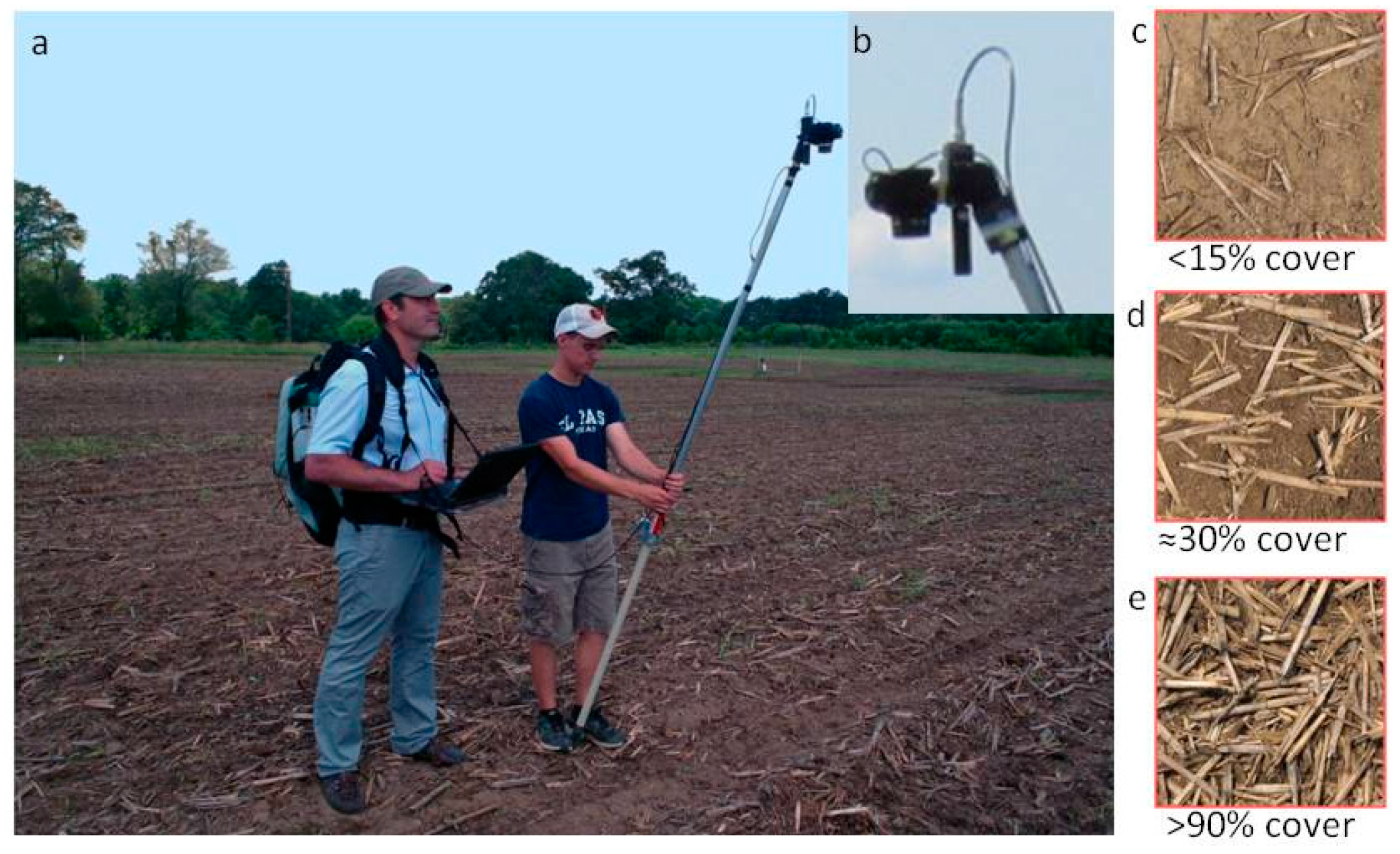
2.2. Field Experiment

The field study was conducted on a portion of the Optimizing Production Inputs for Economic and Environmental Enhancement (OPE3) research site [40], a long-term continuous maize research field on the USDA Henry A. Wallace Beltsville Agricultural Research Center near Beltsville, Maryland (near 39.0320°N, −76.8455°W). The soils are sandy, with Matawan (Table 1) being the majority soil type. Top soil texture was sandy loam to loamy sand. Maize residues were collected from this site.

In mid-July 2014, 10 plots (3-m diameter) were prepared by raking to remove maize residues from the previous crop. Two blocks with five levels of f_R (0, 0.2–0.4, 0.4–0.6, 0.6–0.8, 0.8–1) were established by uniformly distributing maize residues over the soil surface of each plot. The maize residues were mostly stalks that were 0.4–0.8 m long.

Reflectance spectra of 30 scans each were acquired at 10 random locations in each plot with the ASD spectroradiometer (Figure 1). The 18° fore optic of the spectroradiometer and a digital camera were aligned and mounted on a pole at 2.3 m above the soil at a 0° view zenith angle, which resulted in a 0.7-m diameter field of view. One digital image (spatial resolution <1 mm) was acquired for each reflectance spectrum. For calibration, a 46-cm square Spectralon reference panel (Labsphere Inc., North Sutton, NH, USA) was placed in the field of view at 0.6 m from the optics, leveled and measured in the same manner as the scenes at 15–20-min intervals. All spectra were acquired within 2 h of local solar noon under clear sky conditions. Reflectance factors were calculated and corrected for the non-ideal properties of the reference panel [39].

On 25 July 2014, after reflectance spectra were acquired for each plot, one block (5 plots) was uniformly sprinkled with about 5 mm of water to increase the range of moisture content of the maize residues and soil surface. After 1 h, reflectance spectra were acquired from all plots. On the afternoon of 29 July, one block (5 plots) were sprinkled with about 8 mm of water and covered with a polyethylene sheet. The next morning, the plots were uncovered, and reflectance spectra were acquired multiple times as the soils and residues dried. Reflectance spectra were also acquired of a bare soil plot that was progressively covered with saturated crop residues until full coverage was achieved. Overall, 410 field reflectance spectra and digital images were acquired covering a broad range of f_R and scene moisture contents.

The fractions of green vegetation, crop residue and soil in the field of view of the spectroradiometer were determined visually using SamplePoint software [41]. The area viewed by the spectroradiometer was extracted from each image, and a digital grid of crosshairs was superimposed on the extracted image. The numbers of crosshairs that intersected green vegetation, crop residue or soil were counted, and f_R was calculated as the proportion of crop residue points in each image. The number of crosshairs within the field of view of the spectroradiometer was 132. We divided the 410 images among four analysts. When each analyst evaluated the same subset of 10 images, the root mean square error was <4%. Green vegetation was <3% in all images.

Samples of crop residues and the upper 2 cm of soil were acquired for each plot just before the reflectance spectra were acquired. The crop residues were dried at 60 °C, and the soils were dried at 105 °C until stable weight was achieved. Water contents were first expressed on a dry matter basis (g H₂O/g dry residue or soil) and then as relative water content (RWC). The RWC content of each reflectance spectrum within a plot was calculated as the linear combination of the RWC of the residue and soils:

RWC = RWC_S (1 − f_R) + RWC_R (f_R)

(4)

where RWC_S and RWC_R are the relative water contents of soil and crop residue, respectively, f_R is the fraction of residue cover and (1 − f_R) is the soil fraction.

2.3. Data Analysis

Reflectance factors of the soils and crop residues were plotted as a function of wavelength and RWC. In the laboratory experiment, the reflectance of mixed scenes R_(M,λ) with various proportions of crop residues and soils was simulated using linear combinations of the reflectance factors for crop residues and soils [16,20]:

R_(M,λ) = R_(S,λ) (1 − f_R) + R_(R,λ) (f_R)

(5)

where R_(S,λ) and R_(R,λ) are reflectance factors in waveband λ for soils and crop residues, respectively, f_R is the fraction residue cover and (1 − f_R) is the soil fraction. Relative water content of the mixed scenes was calculated using Equation (4).

Reflectance factors were convolved over WorldView-3 and Landsat band passes using the relative spectral response functions to determine equivalent spectral bands [25,26,29]. Spectral indices used for assessing f_R of scenes with varying proportions of crop residues and soils are listed in

Table 2. Spectral bands used for the crop residue cover indices.

Band *	Wavelengths, nm	Residue Index	Equation	Reference
R2.0	2025–2035	Cellulose Absorption Index (CAI)	(1)	[24]
R2.1	2095–2105
R2.2	2200–2210
SWIR6	2185–2225	Shortwave Infrared Normalized Difference Residue Index (SINDRI)	(2)	[10]
SWIR7	2235–2285
OLI6	1570–1650	Normalized Difference Tillage Index (NDTI)	(3)	[32]
OLI7	2110–2290

* R_x.x are hyperspectral bands at the designated wavelengths; SWIR6 and SWIR7 are WorldView-3 bands; and OLI6 and OLI7 are Landsat OLI bands.

.

Changes in slope and intercept of f_R versus each residue index were described by linear and non-linear regression models as functions of RWC for the simulated scenes. In addition, RWC in the field and laboratory was estimated using spectral water indices previously used in the literature or developed in this study (

Table 3. Equations of the spectral indices used to estimate the relative water content and the root mean square error (RMSE) of the linear-plateau model fitted to the data collected in the laboratory experiment.

Equation	Reference	RMSE	Comments
R1.65/R0.85	[33]	0.40	Rx.x reflectance in the hyperspectral 10-nm bands centered at the wavelengths designated by the sub-index in µm
(R0.85 − R1.65)/(R0.85 + R1.65)	[36]	0.31
R1.6/R1.5	This study	0.14
R1.6/R2.0	This study	0.15
R2.2/R2.0	[21]	0.19
SWIR3/SWIR5	This study	0.18	Reflectance in the WorldView, 3 bands
SWIR3/SWIR6	This study	0.17	SWIR3: 1640–1680 nm SWIR5: 2145–2185 nm SWIR6: 2185–2225 nm
OLI5/OLI7	[37]	0.20	Reflectance in the Landsat OLI bands
OLI6/OLI7	[37]	0.19	OLI5:850–880 nm OLI6: 1570–1650 nm OLI7: 2110–2290 nm
(OLI5 − OLI6)/(OLI5 + OLI6)	[38]	0.26
(OLI5 − OLI7)/(OLI5 + OLI7)	[37]	0.20

). The random forest algorithm [42] identified three major clusters of RWC in the field data. The variables included in the algorithm were CAI, SINDRI, NDTI, f_R and RWC. Linear models for predicting f_R as a function of each spectral index were evaluated for each cluster of points. Models for predicting f_R based on the laboratory data were tested with field data.

3. Results and Discussion

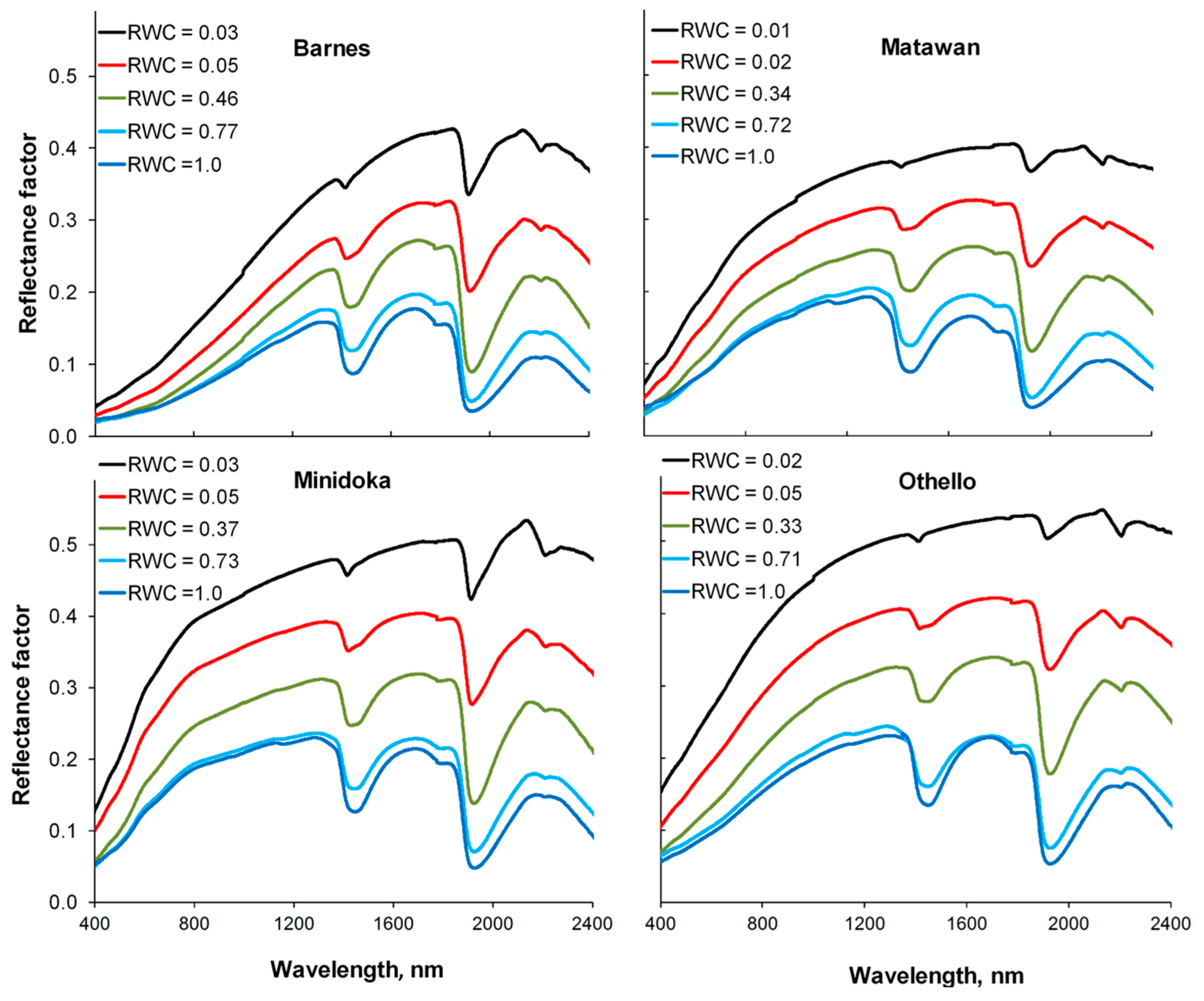
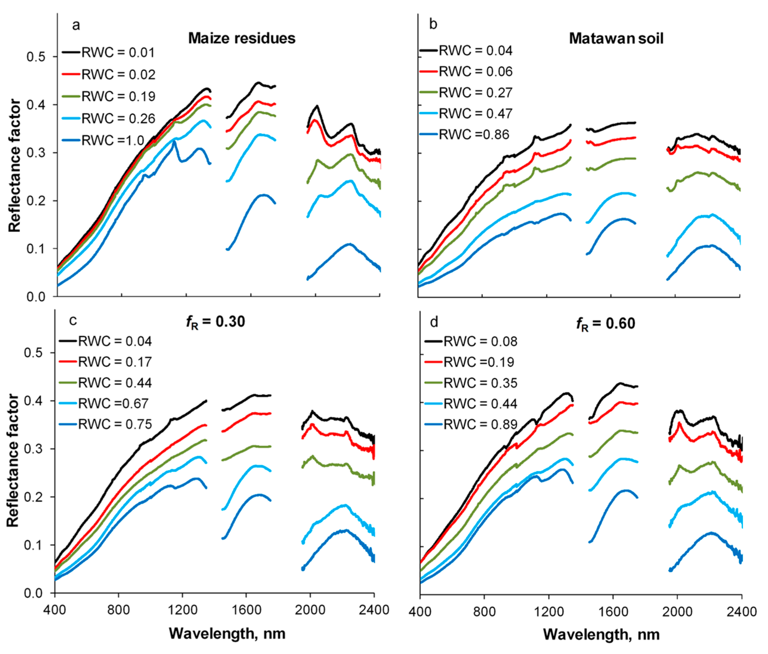
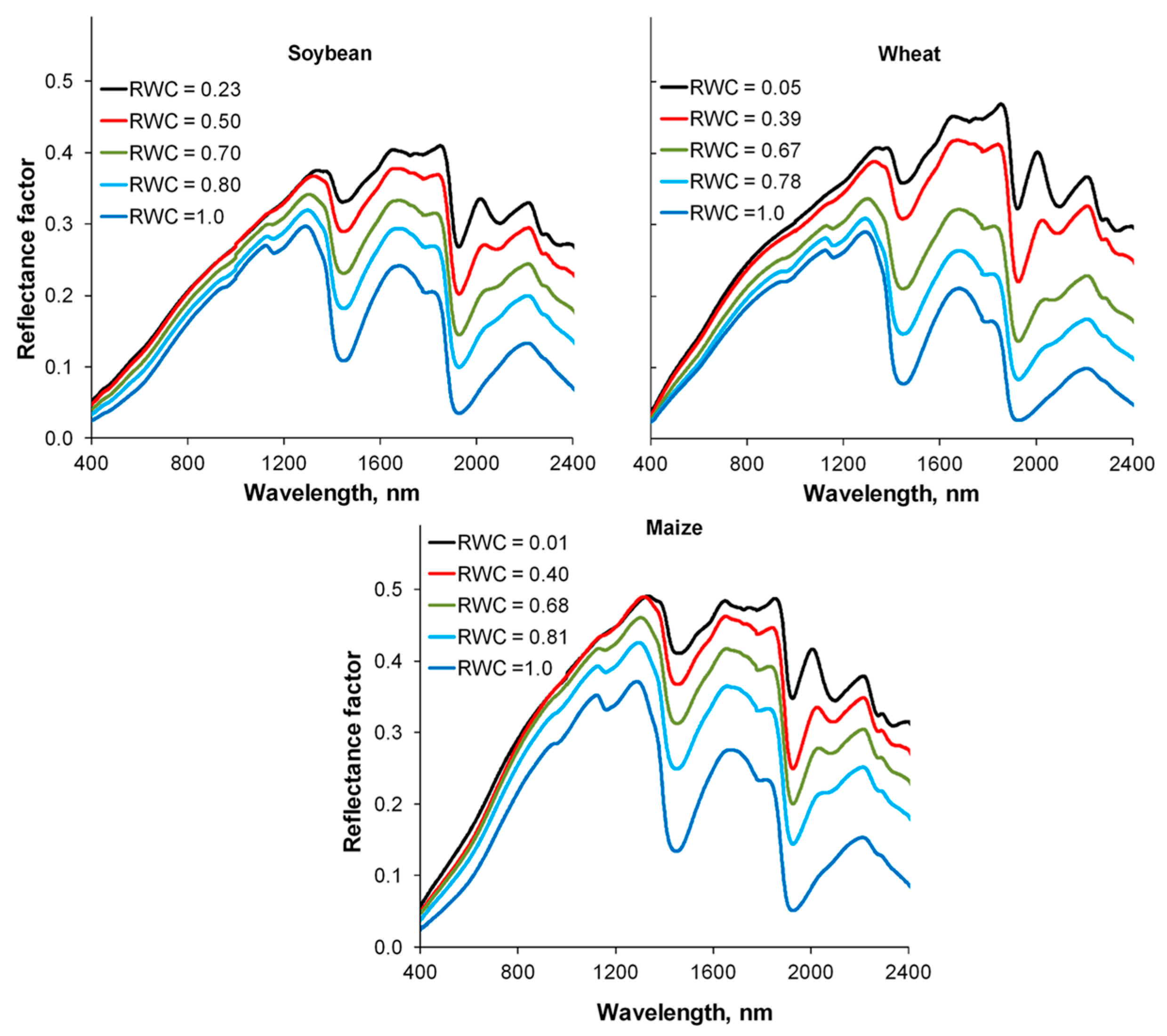
3.1. Lab Reflectance Spectra of Crop Residues and Soils

The effects of water on the reflectance spectra of crop residues and soils are shown in Figure 2 and Figure 3. At low water contents, the absorption feature associated with the −OH bond in the cellulose near 2100 nm [43] is clearly evident in the spectra of crop residues, but is absent in the spectra of soils [24]. The soils have an absorption feature associated with clay minerals near 2200 nm that is absent in the spectra of crop residues.

As water content in the crop residues and soils increased, reflectance across all wavelengths decreased. The well-known water absorption features near 1450 and 1960 nm dominated the reflectance spectra and significantly attenuated the absorption features of cellulose in the crop residues and minerals in the soils [17,18]. Similar changes in reflectance spectra of crop residues and soils as a function of RWC have been reported [16,20].

Water also significantly affected CAI, SINDRI and NDTI for the three crop residues and four soils (Figure 4). As RWC increased, CAI decreased for crop residues, but increased for soils (Figure 4a,d). CAI estimated the depth of the cellulose absorption feature near 2100 nm. Water in the crop residues significantly attenuated the cellulose absorption feature, which resulted in CAI declining as RWC increased. However CAI of the soils increased slightly as RWC increased (Figure 4a,d). As a result, CAI values of the soils and crop residues nearly converged as water contents approached saturation.

For SINDRI, the difference between the soils and crop residues remained significant at all RWC (Figure 4b). The two bands for SINDRI are relatively narrow (40–50 nm) and are located >200 nm from the water absorption future at 1960 nm. As a result, reflectance in bands SWIR6 and SWIR7 for both crop residues and soils decreased as RWC increased, but at slightly different rates (Figure 4e).

The NDTI for soils increased monotonically as RWC increased; however, NDTI for crop residues exhibited two linear phases with a breakpoint near RWC = 0.6 (Figure 4c). For RWC < 0.6, NDTI of the crop residues increased only slightly, but NDTI increased sharply when RWC > 0.6 (Figure 4c). Reflectance of the soils in the OLI6 and OLI7 bands decreased continuously with RWC, but at slightly different rates (Figure 4f), which accounted for the increase in NDTI as a function of RWC (Figure 4c). For the crop residues when RWC < 0.6, reflectance in OLI6 and OLI7 decreased at slightly different rates as RWC increased, but NDTI remained nearly constant. However, when RWC > 0.6, reflectance in both bands decreased sharply, and NDTI increased. Similar patterns for other crop residues and soils were observed, but are not shown. Based on these results, NDTI is capable of assessing crop residue cover when RWC < 0.25 for crop residues and soils. Although NDTI appears capable of assessing crop residue cover when RWC > 0.8, low reflectance values for OLI6 and OLI7 may cause problems.

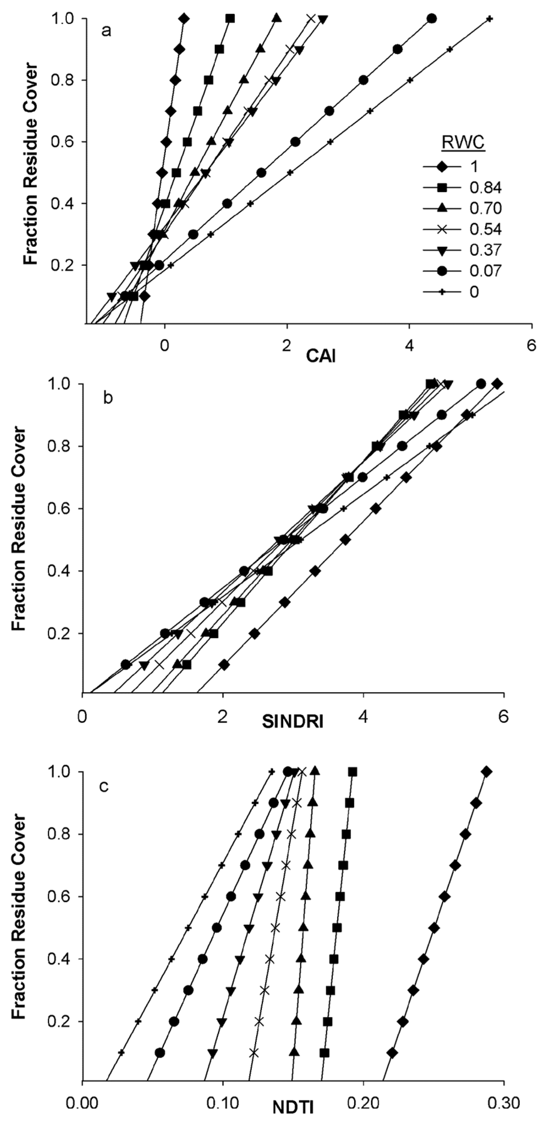
3.2. Simulated Reflectance Spectra of Mixed Scenes

Reflectance spectra of mixed scenes were simulated as linear combinations of the reflectance factors of crop residues and soils using Equation (5), and CAI, SINDRI and NDTI were calculated. The slope of the linear relationship between f_R and CAI was altered by RWC, particularly when RWC was >0.5 (Figure 5a), in agreement with previous observations [16,20]. Both the slope and intercept of f_R vs. CAI were significantly affected by changes in scene RWC (Figure 5a) and were described by exponential models with three parameters (

Table 4. Regression coefficients (mean ± SE), root mean square error of the estimate (RMSE) and adjusted coefficient of determination (Adj. r²) of the models fitted to changes in the slope and the intercept of the percentage of residue cover (f_R) versus the various indices studied due to the RWC of the crop residues and soil (Matawan) mixed scene from the laboratory experiment. The models are plotted in the Supplementary Materials (Figure S1). Coefficient a is the slope and intercept under dry conditions.

Model	Residue	fR Versus Index				RMSE	Adj. r2
		a ± SE	b ± SE	c ± SE	d ± SE
Cellulose Adsorption Index (CAI)
Slope = a + b × exp (c × RWC)	Maize	0.21 ± 0.29	0.001 ± 0.010	8.15 ± 1.08	-	0.055	0.98
	Soybean	0.18 ± 0.02	0.008 ± 0.002	5.52 ± 0.24	-	0.030	0.99
	Wheat	0.14 ± 0.02	0.018 ± 0.004	4.47 ± 0.20	-	0.024	0.99
Intercept = a + b × exp (c × RWC)	Maize	0.20 ± 0.02	0.009 ± 0.008	3.67 ± 0.92	-	0.028	0.95
	Soybean	0.20 ± 0.03	0.029 ± 0.013	3.11 ± 0.41	-	0.025	0.98
	Wheat	0.26 ± 0.02	0.101 ± 0.005	4.09 ± 0.48	-	0.023	0.99
Shortwave Infrared Normalized Difference Residue Index (SINDRI)
RWC < d Slope = (a × (d − RWC) + b × (RWC − RWCmin))/(d − RWCmin) RWC > d Slope = (b × (RWCmax − RWC) + c × (RWC − d))/(RWCmax − d)	Maize	0.17 ± 0.01	0.267 ± 0.028	0.23 ± 0.01	0.88 ± 0.26	0.006	0.97
	Soybean	0.18 ± 0.01	0.286 ± 0.009	0.25 ± 0.01	0.76 ± 0.06	0.013	0.88
	Wheat	0.15 ± 0.02	0.254 ± 0.679	0.22 ± 0.01	0.78 ± 0.69	0.004	0.99
Intercept = a + b × RWC	Maize	0.01 ± 0.02	−0.348 ± 0.026	-	-	0.025	0.97
	Soybean	0.01 ± 0.02	−0.367 ± 0.031	-	-	0.024	0.97
	Wheat	0.01 ± 0.01	−0.358 ± 0.006	-	-	0.005	0.99
Normalized Difference Tillage Index (NDTI)
Slope = a + b × exp (−0.5 × ((RWC − c)/d)2)	Maize	10.6 ± 2.2	52.8 ± 4.1	0.74 ± 0.01	0.12 ± 0.01	3.772	0.97
	Soybean	11.9 ± 5.9	90.9 ± 11.1	0.57 ± 0.02	0.14 ± 0.02	8.704	0.92
	Wheat	6.8 ± 0.8	100.1 ± 1.4	0.48 ± 0.01	0.16 ± 0.94	0.936	0.99
Intercept = a + b × exp (−0.5 × ((RWC − c)/d)2)	Maize	−0.59 ± 0.28	−9.1 ± 0.5	0.77 ± 0.01	0.14 ± 0.01	0.476	0.98
	Soybean	−0.20 ± 1.71	−11.7 ± 2.1	0.61 ± 0.03	0.18 ± 0.05	1.888	0.86
	Wheat	−0.77 ± 0.64	−13.6 ± 1.4	0.51 ± 0.00	0.15 ± 0.02	0.782	0.96

). Corrections for scene RWC were required to accurately assess f_R for all combinations of crop residues and soils. However, we are only showing combinations with Matawan soil for clarity.

The slopes of the linear relationships for f_R vs. SINDRI increased linearly and reached their maxima as RWC exceeded 0.75 and then decreased at saturation (Figure 5b). The intercepts linearly decreased with RWC (Figure 5b; Table 4).

Both the slope and intercept of the linear relationship between f_R and NDTI were significantly altered by changes in RWC (Figure 5c). Initially, both parameters changed little when the scenes were relatively dry (RWC < 0.2), but as RWC increased, both slopes and intercepts changed rapidly (Figure 5c; Table 4), which indicated that NDTI is not reliable for assessing crop residue cover when moisture increases.

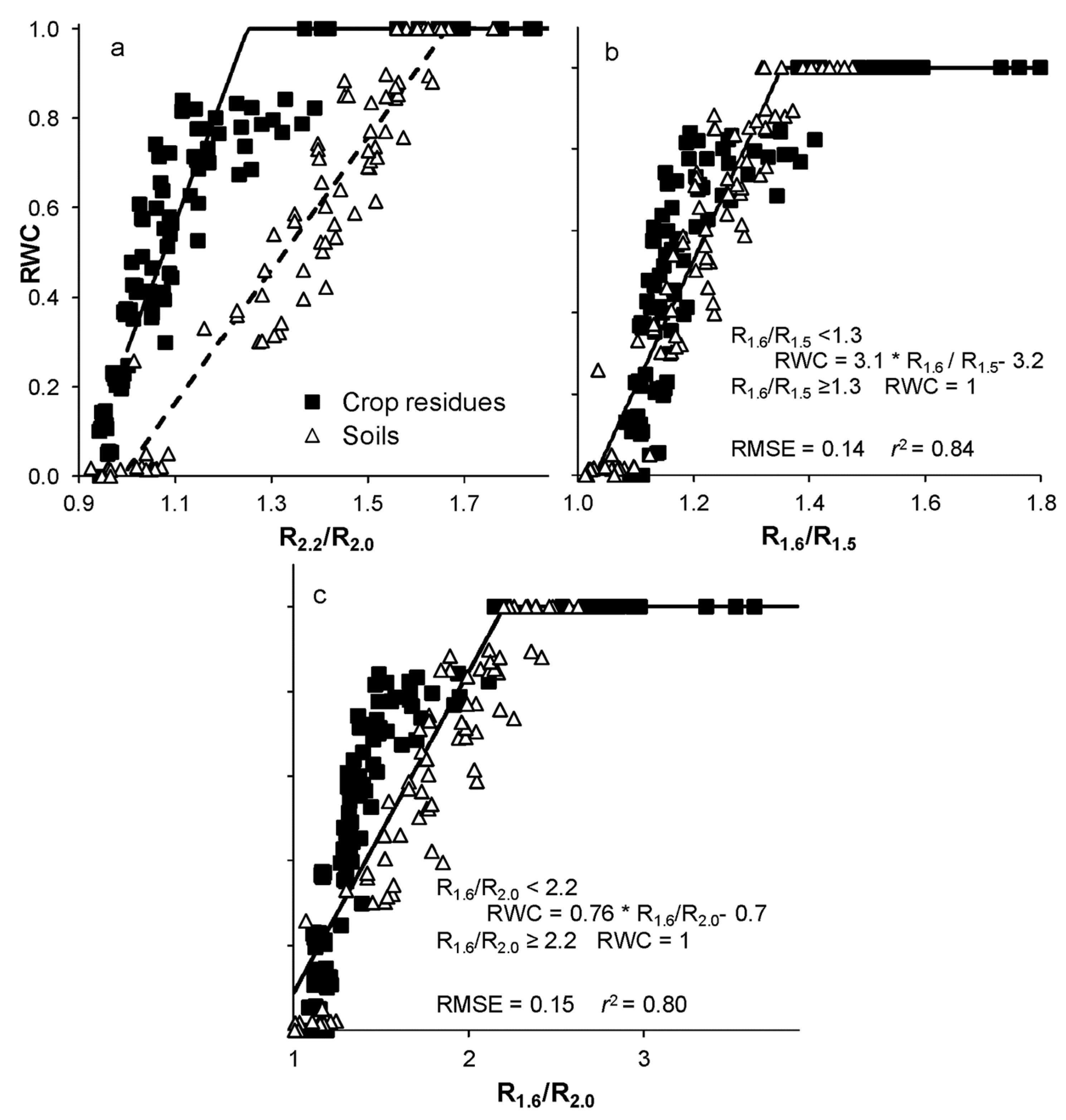
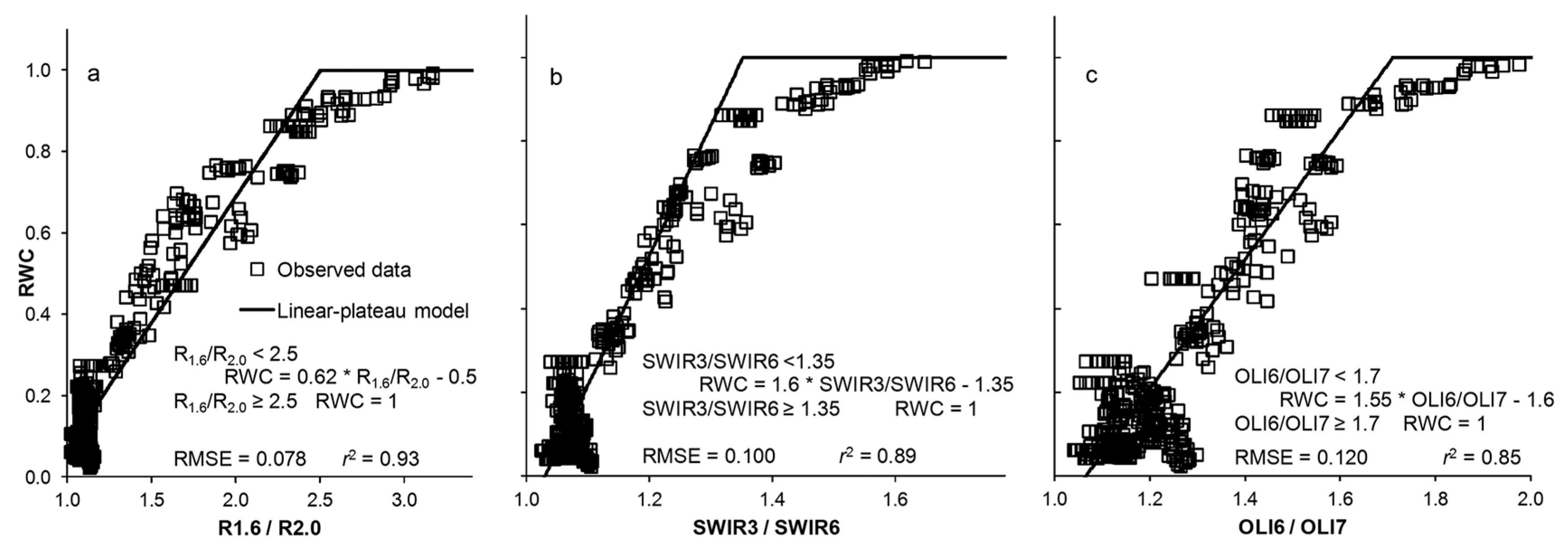
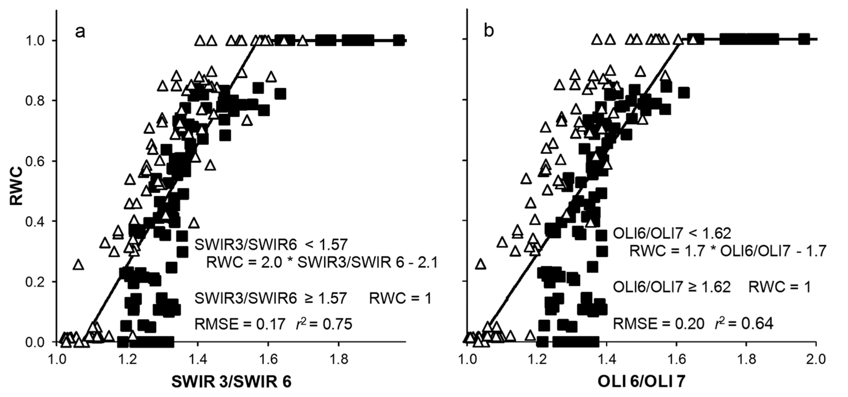
3.3. Spectral Water Indices: RWC Estimation from Lab Equations

Clearly, reliable remotely-sensed estimates of crop residue cover must account for spatial and temporal variations in the RWC of crop residues and soils. However, direct measurements of RWC are impractical for large areas in a timely manner. Thus, spectral water indices that can estimate the spatial and temporal variability of RWC are required. Reflectance in the shortwave infrared region (SWIR) is particularly sensitive to the water content of soils and vegetation [35,44,45]. We examined the ability of several existing and new SWIR spectral water indices to estimate RWC of crop residues and soils. Ideally, the spectral bands used for the water indices would be included in the complement of spectral bands for each satellite sensor. In most cases, RWC was linearly related to the ratio water indices until the soils and crop residues were nearly saturated, i.e., RWC > 0.9 (Figure 6). The linear-, quadratic- and exponential-plateau models significantly fit the data, and the RMSE for the linear-plateau model is shown for comparison purposes (Table 4). Although the reflectance ratio R_2.2/R_2.0 was highly related to the RWC, the relationship differed for soils and crop residues (Figure 6a). Daughtry and Hunt [20] observed that R_2.2/R_2.0 described the changes in the slope of f_R vs. CAI as RWC varied, but did not estimate RWC directly. The reflectance ratios R_1.6/R_1.5 and R_1.6/R_2.0 were equally valuable for the soils and crop residues (Figure 6b,c), which is an advantage, as most agricultural scenes are combinations of soils and crop residues. The indices R_1.6/R_0.8 [33] and the Normalized Difference Infrared Index [36] were also related to RWC, but did not perform as well as R_1.6/R_1.5 and R_1.6/R_2.0 (Table 2).

Because these hyperspectral bands are not available on advanced and broadband multispectral satellite sensors, we also examined water indices that could be calculated using the available bands of current satellite sensors. For estimating RWC, the best relationships were SWIR3/SWIR6 for WorldView-3 and OLI6/OLI7 for Landsat (Table 4; Figure 7). Although the spectral water indices based on satellite bands had larger errors than the narrow band indices for estimating RWC, all were highly significant. Therefore, the moisture conditions for each pixel could be estimated and used to correct the slope and intercept of the equations in Table 4 for assessing residue cover.

3.4. Field Reflectance Spectra and Indices for f_R Assessment

3.4.1. Reflectance Spectra

Representative reflectance spectra of maize residues on the Matawan soil collected in the field at various RWC levels are presented in Figure 8. Atmospheric water absorption features near 1450 and 1960 nm attenuated the incoming solar radiation and were removed.

The absorption feature near 2100 nm remained as the major difference between soil and residue spectra at low water content. As water content in crop residues and soil increased, the reflectance across all wavelengths decreased. In particular, the reflectance at 2030 nm (R_2.0) was reduced with respect to reflectance at 2200 nm (R_2.2), and the cellulose absorption feature near 2100 nm was attenuated as water content increased (Figure 1, Figure 2 and Figure 8). The effects of water on the reflectance spectra measured in the laboratory and in the field were similar. Therefore, correction factors based on the laboratory data should improve our understanding of the field data.

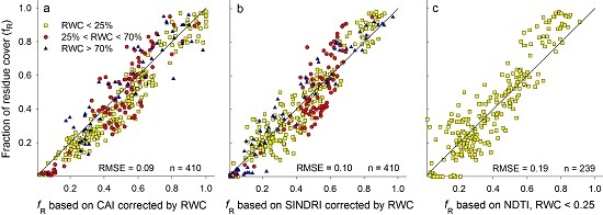
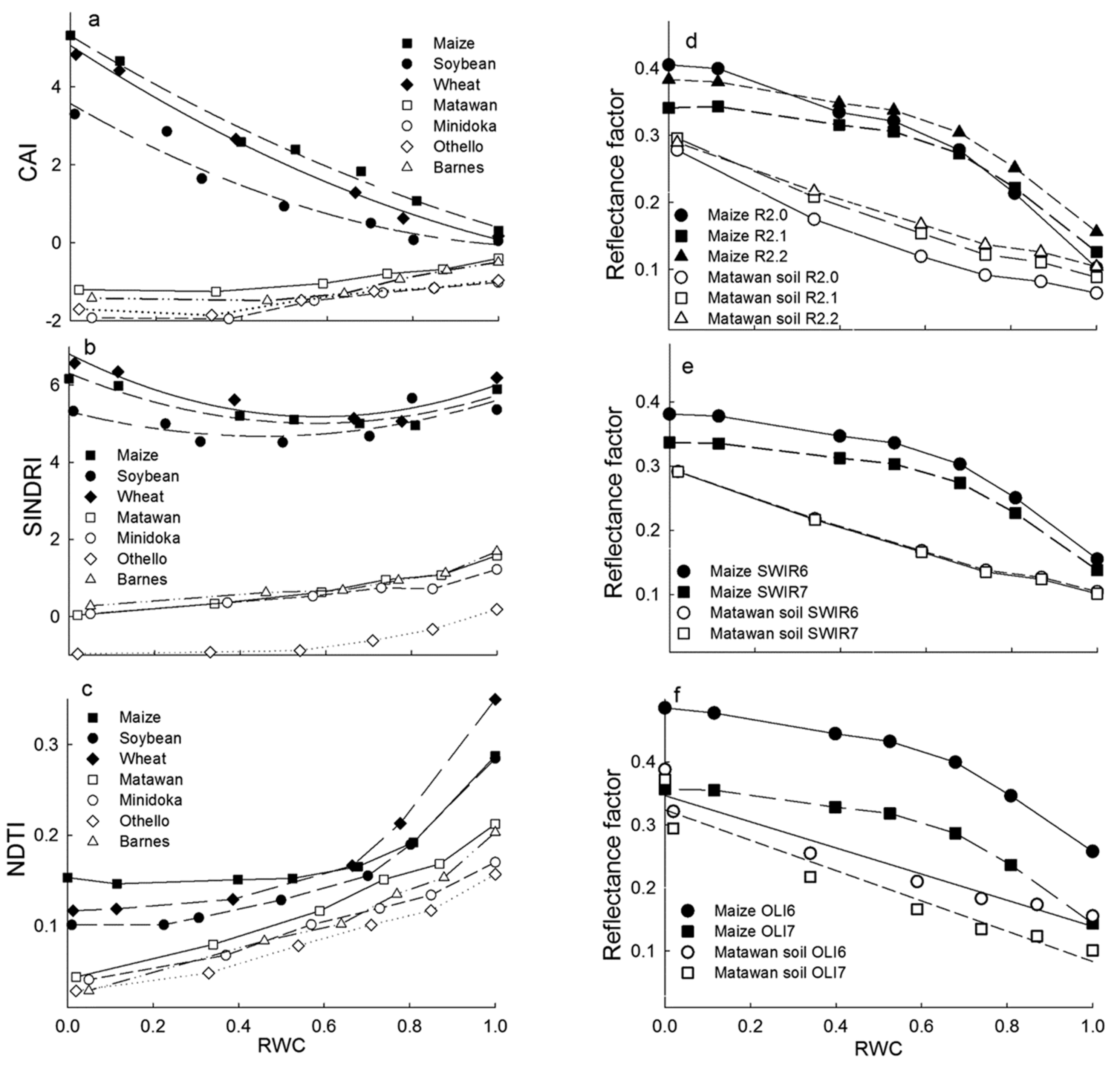
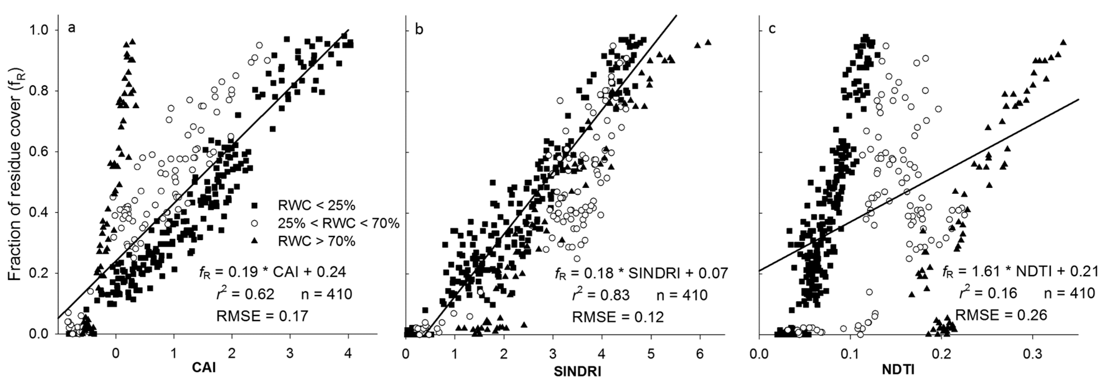
3.4.2. Relationship between f_R and Spectral Indices

When all of the field observations were considered together, the linear regression of f_R and CAI was significant with an adjusted coefficient of determination (Adj. r²) of 0.62 and the RMSE of 0.17 (Figure 9a). However, when the data were grouped based on RWC, highly significant linear relationships were observed between f_R and CAI for each group (

Table 5. Regression coefficients and adjusted coefficient of determination (Adj. r²) of the linear models fitted to the fraction of residue cover measured in the field and the spectral residue indices (CAI, SINDRI and NDTI) when the data were separated into groups based on their RWC.

	Slope	Intercept	Adj. r2	n
Cellulose Absorption Index (CAI)
RWC < 0.25	0.22	0.13	0.95 **	240
0.25 < RWC < 0.70	0.27	0.26	0.88 **	100
RWC > 0.70	1.13	0.56	0.93 **	70
Shortwave Infrared Normalized Difference Residue Index (SINDRI)
RWC < 0.25	0.20	−0.05	0.91 **	240
0.25 < RWC < 0.70	0.17	−0.07	0.76 *	100
RWC > 0.70	0.23	−0.32	0.94 **	70
Normalized Difference Tillage Index (NDTI)
RWC < 0.25	10.13	−0.34	0.85 **	240
0.25 < RWC < 0.70	6.74	−0.31	0.22	100
RWC > 0.70	6.35	−1.09	0.83 **	70

* and ** significant at the 0.05 and 0.01 probability levels, respectively.

). Slopes and intercepts of the linear regressions increased with RWC content, as was observed in the laboratory experiment.

The linear regression for f_R and SINDRI was significant with an adjusted r² of 0.83 when all of the observations were considered together (Figure 9b). However, when the data were separated into three groups based on RWC, their r² improved (Table 5). The adjusted r² of the intermediate class declined slightly, but was significant. Slopes and intercepts followed trends similar to the results from the laboratory experiment. The field data also confirmed that variations in RWC had less of an impact on SINDRI than CAI.

The linear regression for f_R and NDTI was not significant when all of the observations were considered together (Figure 9c). However, when they were separated into classes based on RWC, significant linear relationships were observed for the driest and wettest classes (Table 5). The linear regression for the intermediate RWC class was not significant. This agrees with the results from the laboratory experiment, which showed that NDTI was insensitive to f_R when RWC was >0.3 (Figure 4c).

In summary, the responses of spectral crop residue indices to RWC were similar in both laboratory and field experiments. Clearly, estimates of scene RWC are required to reliably assess f_R regardless of which crop residue spectral index is used. We hypothesize that models developed to predict f_R using the laboratory data (Table 4; Figure 4) should predict f_R for the field experiment.

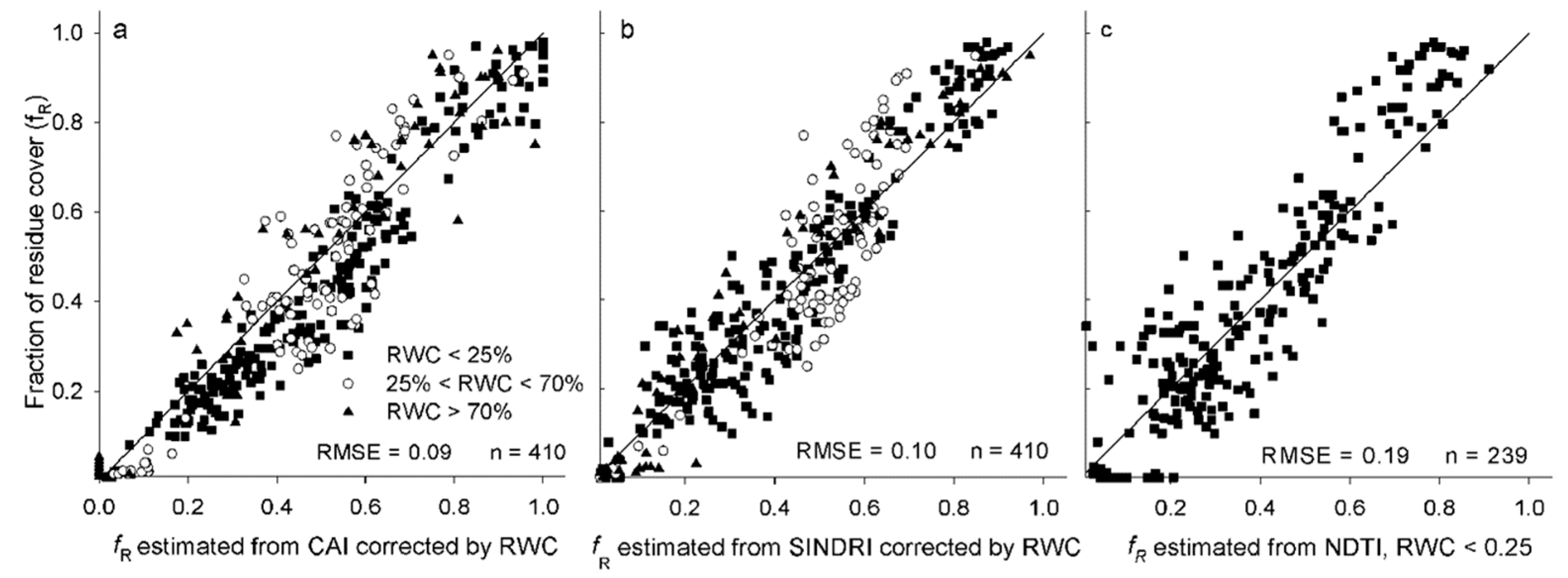
3.5. Spectral Water Indices and Prediction of f_R (Residue Cover Spectral Index, Water Spectral Index)

Spectral water indices estimated scene RWC using narrow spectral bands (Figure 6) or relatively broad satellite bands (Figure 7) from the SWIR region. Adjusted r² was >0.92, and RMSE was ≤0.10 for RWC predicted by the equations from the laboratory experiment and the RWC observed in the field (

Table 6. Root mean square error (RMSE) and adjusted coefficient of determination (Adj. r²) for the relative water content (RWC) measured in the field and estimated by the equations from the laboratory experiment, as a function of the water indexes based on narrow bands (Figure 6) or on satellite bands (Figure 7) extracted from the reflectance spectra measured in the field (n = 410).

	RMSE	Adj. r2
Water indices based on narrow bands
R2.2/R2.0	0.100	0.93
R1.6/R1.5	0.099	0.93
R1.6/R2.0	0.096	0.94
Water indices based on satellite bands
SWIR 3/SWIR 6	0.151	0.88
OLI6 /OLI7	0.177	0.84

). This is particularly important because the spectral water indices were developed for different soils and crop residues. Both linear-plateau and quadratic models fit the observed data well (

Table 7. Regression coefficients, RMSE and adjusted coefficient of determination (Adj. r²) for the RWC of field measurements as a function of the water indices based on narrow bands (Figure 6) or on satellite-like bands extracted from the reflectance spectra measured in the field (n = 410).

Spectral Water Index	Linear-Plateau Model †
	a	b	c	RMSE	Adj. r2
Water indices based on narrow bands
R2.2/R2.0	−1.1	1.23	1.66	0.081	0.92
R1.6/R1.5	−2.6	2.57	1.41	0.083	0.93
R1.6/R2.0	−0.5	0.62	2.50	0.078	0.93
Water indices based on satellite bands
SWIR 3/SWIR 6	−1.7	1.60	1.69	0.100	0.89
OLI6 /OLI7	−1.6	1.55	1.71	0.120	0.85

^† Linear-plateau model: if water index > c, RWC = 1; else, RWC = a + b.

; Figure 10). Scene RWC was also predicted using the water indices based on satellite spectral bands (Table 6). The relationships were highly significant, and the RMSE was <0.18 (Table 6). Field measurements of RWC were also highly correlated with the water indices extracted from the field reflectance spectra (Table 7; Figure 10).

Finally, the multivariate linear models (Figure 5; Table 4) predicted f_R using field reflectance spectra are shown in Figure 11. For CAI, the multivariate model adjusted the slope and intercept for changes in scene RWC with the narrow band spectral water indices and reduced the RMSE to <0.1 (

Table 8. RMSE of the fraction of residue cover observed in the field and estimated from the multivariate linear model from the laboratory experiment (Table 4) based on CAI, SINDRI and NDTI, when the relative water content was estimated from various spectra water indices based on narrow or broad bands extracted from the reflectance spectra measured in the field. The RMSE for NDTI considering only data with RWC < 0.25 or RWC < 0.50 are also included.

	R2.2/R2.0	R1.6/R1.5	R1.6/R2.0	SWIR3/SWIR6	OLI6/OLI7	Without RWC Correction	n
CAI	0.10	0.09	0.10	0.11	0.12	0.17	410
SINDRI	0.11	0.10	0.10	0.10	0.11	0.12	410
NDTIall values	0.31	0.31	0.32	0.34	0.34	0.26	410
NDTIRWC<0.50	0.21	0.21	0.22	0.24	0.25	0.25	305
NDTIRWC<0.25	0.18	0.18	0.19	0.19	0.19	0.21	239

; Figure 11a).

For SINDRI, the multivariate linear models modestly reduced RMSE from 0.12 down to 0.10–0.11 (Table 8; Figure 11b), reinforcing that SINDRI is largely independent of scene RWC. The reduction was similar for all of the spectral water indices.

Predicting field f_R using the NDTI multivariate linear model had a large RMSE (>0.30) because of the difficulty of correcting the NDTI when the RWC was between 0.5 and 0.7 (Table 8). When scene RWC was estimated using the OLI6/OLI7 index, the RMSE was 0.34. Thus, the reliability of NDTI to predict crop residue cover is limited when variations in scene moisture conditions are likely. However, when field conditions are relatively dry (RWC < 0.25), the RMSE was 0.19 for NDTI predicted field f_R (Table 8; Figure 11c).

4. General Discussion

In summary, when conditions were dry, crop residue cover was linearly related to each of the three spectral residue indices. However, when relative water content of crop residues and soils varied, estimates of crop residue cover were adversely affected. Spectral water indices were developed to estimate scene relative water content. Pairs of spectral indices were used, one for relative water content and another for crop residue cover; the overall accuracy of crop residue cover estimates when moisture conditions varied.

Both slope and intercept of the f_R vs. CAI were altered by changes in water content under laboratory conditions [16,20]. In this study, we showed that the slopes and the intercepts of the f_R vs. CAI followed similar trends for both laboratory and field conditions, confirming that corrections based on moisture conditions significantly improved the ability of CAI to predict crop residue cover. However, the use of CAI as an index for f_R at regional scales is limited by the lack of suitable hyperspectral remote sensing satellite systems. Hyperion data have been used to calculate CAI and to estimate crop residue cover for test sites in Iowa and Indiana [46,47]. However, the narrow swath width of Hyperion images cannot provide the wall-to-wall coverage needed for regional scale monitoring.

Advanced multispectral sensors with relatively narrow shortwave infrared bands, such as WorldView-3, are alternatives to hyperspectral imaging spectrometers. Our results showed that f_R estimated using SINDRI is less sensitive to variations in scene moisture conditions than f_R estimated with CAI or NDTI. Corrections based on scene moisture conditions slightly improved the ability of SINDRI to predict crop residue cover.

Variations in scene moisture conditions adversely affected f_R estimated using NDTI. Both the slope and intercept of the f_R vs. NDTI regression were significantly altered by variations in scene moisture conditions. Nevertheless, NDTI has been used successfully to distinguish a few broad tillage classes [32,48]. These studies typically evaluated test sites within a single Landsat image. Thus, variations in moisture conditions were probably small and did not significantly alter classification accuracy. Other studies [28,49] have used multi-temporal Landsat images to classify tillage intensity. Gelder et al. [49] selected Landsat images acquired more than two days after precipitation events, which allowed the surface layer to dry for most soils. In contrast, we created broad ranges of scene relative water contents to test the robustness of NDTI for estimating crop residue cover. Under relatively dry (RWC < 0.25) conditions and possibly very wet (RWC > 0.70) conditions, the regressions of f_R vs. NDTI were significant. For these very wet conditions, reflectance in the shortwave infrared bands of Landsat is significantly attenuated by water, and the spectral indices must be used with caution. However, NDTI was not a suitable predictor of f_R for intermediate values of RWC. Thus, assessments of the scene water contents are particularly crucial for estimating f_R using NDTI.

In the field experiment, some of the unexplained variability was probably associated with the experimental protocol for determining residue cover and RWC. The accuracy of SamplePoint measurements to determine ground-cover under field conditions ranges from 92%–98% depending on the quality of the image analyzed [41]. Determining the water content of soil and residue samples is associated with some uncertainty, as the moisture distribution is not homogenous and is affected by soil texture and litter composition [50,51]. Considering this unexplained variability inherent to the field dataset, the accuracy attained (RMSE = 0.09–0.12) when using the equations based on CAI and SINDRI to predict f_R was very high.

In our field experiment, the soil, maize residues and water contents were quite uniform. Within any real agricultural scene, variations in topography, soil roughness, soil texture, green vegetation cover and precipitation affect moisture conditions and spectral reflectance. Therefore, these correlations to estimate RWC in a scene should be used with caution. Additional information about the local soil reflectance and crop type may be useful for estimating scene moisture conditions.

Baird and Baret [52] proposed the CRIM (Crop Residue Index Multiband) method for estimating crop residue cover, which is based on the distance between the soil line and the residue line. In our experiment (data not shown), the contrasts between the soil and residue lines for pairs of visible (OLI4), near infrared (OLI5) and SWIR (OLI6 and OLI7) were very low, which limited the accuracy of the relationship between CRIM and the crop residue cover.

Current hyperspectral sensors (e.g., Hyperion and EnMAP) and advanced multispectral sensors (e.g., WorldView-3) have narrow swaths and are well suited for studying episodic events, but do not have the capacity to map large areas in a timely manner [25]. Therefore, the challenge is how to best use a few hyperspectral and/or advanced multispectral images and many multispectral images (e.g., Landsat, Sentinel-2) to produce regional surveys and maps of crop residue cover and tillage intensity. For example, a simple robust method for quantitatively mapping the fractions of photosynthetic vegetation, non-photosynthetic vegetation and bare soil was developed using Hyperion and MODIS data [52]. The three fractions were successfully mapped over large areas of Australian savannas with daily MODIS data. However, the relatively coarse spatial resolution of MODIS data (i.e., 250–1000 m) would be a limitation for assessing crop residue cover and tillage intensity in agricultural regions with many fields and diverse crops. Another promising example is the Spatial Temporal Adaptive Reflectance Fusion Model (STARFM [53,54]), which combines Landsat and MODIS reflectance data to produce composite images with the spatial resolution of Landsat and the temporal resolution of MODIS. These fused Landsat-MODIS images potentially could provide reliable temporal profiles of NDTI for estimating crop residue cover and soil tillage intensity using the minNDTI approach [28].

5. Conclusions

Each of the spectral residue indices accurately estimated crop residue cover when scene moisture conditions were relatively dry (i.e., relative water content (RWC) <0.25). However, when scene moisture conditions varied from dry to wet, Shortwave Infrared Normalized Difference Residue Index (SINDRI) was the most robust of the three indices without any corrections for moisture. Spectral water indices were evaluated and sufficiently characterized scene water conditions. Pairs of spectral indices—one for scene moisture and one for crop residue cover—improved the overall accuracy of both the Cellulose Absorption Index (CAI) and SINDRI to estimate f_R when scene moisture conditions varied. The Normalized Difference Tillage Index (NDTI) should be used only when scene conditions are relatively dry (RWC < 0.25). These remotely-sensed indices will support mapping broad soil tillage intensity categories (i.e., intensive tillage = f_R < 0.15; reduced tillage = 0.15–0.30; conservation tillage = f_R > 0.30) of the USDA (United States Department of Agriculture) and the ECAF (European Conservation Agriculture Federation).

References

1. Delgado, J.A. Crop residue is a key for sustaining maximum food production and for conservation of our biosphere. J. Soil Water Conserv. 2010, 65, 111–116. [Google Scholar] [CrossRef]
2. Lal, R.; Kimble, J.M.; Follett, R.F.; Cole, C.V. The Potential of U.S. Cropland to Sequester Carbon and Mitigate the Greenhouse Effect; Lewis Publishers: Boca Raton, FL, USA, 1999; p. 128. [Google Scholar]
3. Izaurralde, R.C.; Williams, J.R.; McGill, W.B.; Rosenberg, N.J.; Quiroga Jakas, M.C. Simulating soil C dynamics with EPIC: Model description and testing against long-term data. Ecol. Model. 2006, 192, 362–384. [Google Scholar] [CrossRef]
4. Gassman, P.W.; Reyes, M.; Green, C.H.; Arnold, J.G. The Soil and Water Assessment Tool: historical development, applications, and future directions. Trans. ASABE 2007, 50, 1211–1250. [Google Scholar] [CrossRef]
5. CTIC Crop. Residue Management Survey System; Conservation Technology Information Center: West Lafayette, IN, USA, 2015. [Google Scholar]
6. Morrison, J.E., Jr.; Huang, C.H.; Lightle, D.T.; Daughtry, C.S.T. Residue measurements techniques. J. Soil Water Conserv. 1993, 48, 479–483. [Google Scholar]
7. Laflen, J.M.; Ameniya, M.; Hintz, E.A. Measuring crop residue cover. J. Soil Water Conserv. 1981, 36, 341–343. [Google Scholar]
8. Corak, S.J.; Kaspar, T.C.; Meek, D.W. Evaluating methods for measuring residue cover. J. Soil Water Conserv. 1993, 48, 700–704. [Google Scholar]
9. Thoma, D.P.; Gupta, S.C.; Bauer, M.E. Evaluation of optical remote sensing models for crop residue cover assessment. J. Soil Water Conserv. 2004, 59, 224–233. [Google Scholar]
10. Serbin, G.; Hunt, E.R., Jr.; Daughtry, C.S.T.; Doraiswamy, P.C. An improved ASTER index for remote sensing of crop residue. Remote Sens. 2009, 1, 971–991. [Google Scholar] [CrossRef]
11. Zheng, B.; Campbell, J.B.; de Beurs, K.M. Remote sensing of crop residue cover using multi-temporal Landsat imagery. Remote Sens. Environ. 2012, 117, 111–183. [Google Scholar] [CrossRef]
12. Huete, A.R. Soil influences in remotely sensed vegetation-canopy spectra. In Theory and Applications of Optical Remote Sensing; Asrar, G., Ed.; John Wiley & Sons Inc.: New York, NY, USA, 1989; pp. 107–141. [Google Scholar]
13. Brown, D.J.; Schepherd, K.D.; Walsh, M.G.; Mays, M.D.; Reinsch, T.G. Global soil characterization with VNIR diffuse reflectance spectroscopy. Geoderma 2006, 132, 273–290. [Google Scholar] [CrossRef]
14. Daughtry, C.S.T.; Serbin, G.; Reeves, J.B.; Doraiswamy, P.C.; Hunt, E.R., Jr. Spectral reflectance of wheat residue during decomposition and remotely sensed estimates of residue cover. Remote Sens. 2010, 2, 416–431. [Google Scholar] [CrossRef]
15. Nagler, P.L.; Daughtry, C.S.T.; Goward, S.N. Plant litter and soil reflectance. Remote Sens. Environ. 2000, 71, 207–215. [Google Scholar] [CrossRef]
16. Wang, C.K.; Pan, X.Z.; Liu, Y.; Li, Y.L.; Shi, R.; Zhou, R.; Xie, X.L. Alleviating moisture effects on remote Sensing estimation of crop residue cover. Agron. J. 2013, 105, 967–976. [Google Scholar] [CrossRef]
17. Kokaly, R.F.; Clark, R.N. Spectroscopic determination of leaf biochemistry using band-depth analysis of absorption features and stepwise multiple linear regression. Remote Sens. Environ. 1999, 67, 267–287. [Google Scholar] [CrossRef]
18. Curran, P.J. Remote sensing of foliar chemistry. Remote Sens. Environ. 1999, 30, 271–278. [Google Scholar] [CrossRef]
19. Daughtry, C.S.T.; Hunt, E.R., Jr.; Doraiswamy, P.C.; McMurtrey, J.E., III. Remote sensing the spatial distribution of crop residues. Agron. J. 2005, 97, 864–871. [Google Scholar] [CrossRef]
20. Daughtry, C.S.T.; Hunt, E.R., Jr. Mitigating the effects of soil and residue water contents on remotely sensed estimates of crop residue cover. Remote Sens. Environ. 2008, 112, 1647–1657. [Google Scholar] [CrossRef]
21. USGS. Earth Observing 1 (EO-1): Sensors—Hyperion. Available online: http://eo1.usgs.gov/hyperion.php (accessed on 9 June 2016).
22. EnMap. EnMap Hyperspectral Imager. Available online: http://www.enmap.org/ (accessed on 9 June 2016).
23. Daughtry, C.S.T. Discriminating crop residues from soil by shortwave infrared reflectance. Agron. J. 2001, 93, 125–131. [Google Scholar] [CrossRef]
24. Goward, S.N.; Arvindson, T.; Williams, D.L.; Irish, R.; Irons, J.R. Moderate Spatial Resolution Optical Sensors. In The Sage Handbook of Remote Sensing; Warner, T.A., Ed.; Sage Publications: Thousand Oaks, CA, USA, 2009; pp. 123–138. [Google Scholar]
25. SIC. Satellite Imaging Corporation. Available online: http://www.satimagingcorp.com/satellite-sensors/worldview-3/ (accessed on 9 June 2016).
26. Abrams, M. The Advanced Spaceborne Thermal Emission and Reflection Radiometer (ASTER): Data products for the high spatial resolution imager on NASA’s Terra platform. Int. J. Remote Sens. 2000, 21, 847–859. [Google Scholar] [CrossRef]
27. Bannari, A.; Pacheco, A.; Staenz, K.; McNairn, H.; Omari, K. Estimating and Mapping Crop Residue Cover in Agricultural Lands Using Hyperspectral and IKONOS data. Remote Sens. Environ. 2006, 104, 447–459. [Google Scholar] [CrossRef]
28. Zheng, B.; Campbell, J.; Serbin, G.; Daughtry, C.S.T. Multi-temporal remote sensing of crop residue cover and tillage practices: A validation of the minNDTI strategy in the United States. J. Soil Water Conserv. 2013, 68, 120–131. [Google Scholar] [CrossRef]
29. NASA. International Space Station. Available online: http://www.nasa.gov/mission_pages/landsat/main (accessed on 9 June 2016).
30. European Space Agency. Available online: http://www.esa.int/Our_Activities/Observing_the_Earth/Copernicus/Sentinel-2 (accessed on 9 June 2016).
31. McNairn, H.; Protz, R. Mapping corn residue cover on agricultural fields in Oxford County, Ontario using Thematic Mapper. Can. J. Remote Sens. 1993, 19, 152–158. [Google Scholar] [CrossRef]
32. Van Deventer, A.P.; Ward, A.D.; Gowda, P.H.; Lyon, J.G. Using Thematic Mapper Data to Identify Contrasting Soil Plains and Tillage Practices. Photogramm. Eng. Remote Sens. 1997, 63, 87–93. [Google Scholar]
33. Hunt, E.R.; Rock, B.N. Detection of changes in leaf water content using near- and middle-infrared reflectances. Remote Sens. Environ. 1989, 30, 43–54. [Google Scholar]
34. Hunt, E.R., Jr.; Daughtry, C.S.T.; Li, L. Feasibility of estimating leaf water content using spectral indices from WolrdView-3’s near-infrared and shortwave infrared bands. Int. J. Remote Sens. 2016, 37, 388–402. [Google Scholar] [CrossRef]
35. Lobell, D.; Asner, G.P. Moisture effects on soil reflectance. Soil Sci. Soc. Am. J. 2002, 66, 722–727. [Google Scholar] [CrossRef]
36. Hardisky, M.A.; Klemas, V.; Smart, R.M. The influence of soil-salinity, growth form, and leaf moisture on the spectral radiance of Spartina alterniflora canopies. Photogramm. Eng. Remote Sens. 1983, 49, 77–83. [Google Scholar]
37. Gao, Y.; Walker, J.P.; Allahmoradi, M.; Monerris, A.; Ryu, D.; Thomas, J.J. Optical sensing of vegetation water content: A synthesis study. IEEE J. Sel. Top. Appl. 2015, 8, 1456–1464. [Google Scholar]
38. Pyne, S.J.; Andrews, P.L.; Laven, R.D. Introduction to Wildland Fire; John Wiley & Son Publishing: New York, NY, USA, 1996; p. 769. [Google Scholar]
39. Robinson, B.F.; Biehl, L.L. Calibration procedures for measurement of reflectance factor in remote sensing field research. Soc. Photo-Opt. Instrum. 1979, 196, 16–26. [Google Scholar]
40. Gish, T.J.; Walthall, C.L.; Daughtry, C.S.T.; Kung, K.-J.S. Using soil moisture and spatial yield patterns to identify subsurface flow pathways. J. Environ. Qual. 2005, 34, 274–286. [Google Scholar] [CrossRef] [PubMed]
41. Booth, D.T.; Cox, S.E.; Berryman, R.D. Precision measurements from very-large scale aerial digital imagery. Environ. Monit. Assess. 2006, 112, 293–307. [Google Scholar] [CrossRef] [PubMed]
42. Liaw, A.; Wiener, M. Classification and regression by random forest. R. News 2002, 2, 18–22. [Google Scholar]
43. Murray, I.; Williams, P.C. Chemical Principles of Near-Infrared Technology. In Near-Infrared Technology in the Agricultural and Food Industries; Williams, P.C., Norris, K., Eds.; American Association Cereal Chemists: St. Paul, MN, USA, 1988. [Google Scholar]
44. Whiting, M.L.; Li, L.; Ustin, S. Predicting water content using Gaussian model on soil spectra. Remote Sens. Environ. 2004, 89, 535–552. [Google Scholar] [CrossRef]
45. Dematte, J.A.M.; Soussa, A.A.; Alves, M.C.; Nanni, M.R.; Fiorio, P.R.; Campos, R.C. Determining soil water status and other soil characteristics by spectral proximal sensing. Geoderma 2006, 135, 179–195. [Google Scholar] [CrossRef]
46. Daughtry, C.S.T.; Doraiswamy, P.C.; Hunt, E.R.; Stern, A.J.; McMurtrey, J.E., III; Prueger, J.H. Remote sensing of crop residue cover and soil tillage intensity. Soil Tillage Res. 2006, 91, 101–108. [Google Scholar] [CrossRef]
47. Galloza, M.S.; Crawford, M.M.; Heathman, G.C. Crop residue modeling and mapping using Landsat, ALI, Hyperion, airborne remote sensing data. IEEE J. Sel. Top. Appl. 2013, 6, 446–456. [Google Scholar] [CrossRef]
48. Sullivan, D.G.; Strickland, T.C.; Masters, M.H. Satellite mapping of conservation tillage adoption in the Little River experimental watershed, Georgia. J. Soil Water Conserv. 2008, 63, 112–119. [Google Scholar] [CrossRef]
49. Gelder, B.K.; Kaleita, A.L.; Cruse, R.M. Estimating Mean Field Residue Cover on Midwestern Soils Using Satellite Imagery. Agron. J. 2009, 101, 635–643. [Google Scholar] [CrossRef]
50. Quemada, M.; Cabrera, M.L. Characteristic moisture curves and maximum water content of two crop residues. Plant. Soil 2002, 238, 295–299. [Google Scholar] [CrossRef]
51. Quemada, M.; Cabrera, M.L. Predicting crop residue decomposition using moisture adjusted time scales. Nutr. Cycl. Agroecosyst. 2004, 70, 283–291. [Google Scholar] [CrossRef]
52. Guerschman, J.P.; Hill, M.J.; Renzullo, L.J.; Barrett, D.J.; Marks, A.S.; Botha, E.J. Estimating fractional cover of photosynthetic vegetation, non-photosynthetic vegetation and bare soil in the Australian tropical savanna region upscaling the EO-1 Hyperion and MODIS sensors. Remote Sens. Environ. 2009, 113, 928–945. [Google Scholar] [CrossRef]
53. Gao, F.; Masek, J.G.; Hall, J.; Schwaller, M. On the blending of the Landsat and MODIS surface reflectance: predicting daily Landsat surface reflectance. IEEE Trans. Geosci. Remote 2006, 44, 2207–2218. [Google Scholar]
54. Gao, F.; Masek, J.; Wolfe, R.; Huang, C. Building consistent medium resolution satellite data set using moderate resolution imaging spectroradiometer products as reference. J. Appl. Remote Sens. 2010, 4, 043526. [Google Scholar]
Figure 1. Photographs of: (a) the image and spectra acquisition from the research field in Beltsville, MD, USA; (b) detail of the digital camera and the 18° fore optic of the spectroradiometer aligned; and examples of the soil surface covered by (c) <15%; (d) 30% and (e) >90% of crop residues.
Remotesensing 08 00660 g001
Figure 2. Reflectance spectra of three crop residues at various relative water contents (RWC) collected in the laboratory.
Remotesensing 08 00660 g002
Figure 3. Reflectance spectra of four soils at various relative water contents (RWC) collected in the laboratory.
Remotesensing 08 00660 g003
Figure 4. Changes in CAI (a); SINDRI (b) and NDTI (c) of three crop residues and four soils and bands R2.0, R2.1 and R2.2 (d); bands SWIR6 and SWIR7 (e) and OLI6 and OLI7 (f) of maize residue as a function of relative water content (RWC) based on the spectra collected in the laboratory.
Remotesensing 08 00660 g004
Figure 5. Residue cover as a function of (a) CAI; (b) SINDRI and (c) NDTI for simulated scenes of maize residues on Matawan soil for RWC ranging from dry to saturated.
Remotesensing 08 00660 g005
Figure 6. RWC for crop residues and soils as a function of three narrow band reflectance ratios: (a) R2.2/R2.0; (b) R1.6/R1.5; and (c) R1.6/R2.0. The bands R1.5, R1.6, R2.0 and R2.2 are 10-nm bands centered at 1500, 1600, 2030 and 2200 nm, respectively.
Remotesensing 08 00660 g006
Figure 7. RWC for crop residues and soils as a function of two water indices based on satellite band ratios: (a) SWIR3/SWIR6 for WorldView-3; and (b) OLI6/OLI7 for Landsat. The spectral bands are: SWIR3 (1640–1680 nm), SWIR6 (2185–2225 nm), OLI6 (1570–1650 nm) and OLI7 (2110–2290 nm).
Remotesensing 08 00660 g007
Figure 8. Field reflectance spectra of (a) maize residues; (b) Matawan soil; (c) 0.30 residue cover (fR) and (d) 0.60 fR at various RWC. Maize residue spectra are from scenes with fR > 0.95, whereas Matawan soil spectra are scenes with fR < 0.02. The remaining two graphs represent scenes with maize fR = 0.30 ± 0.03 and fR = 0.60 ± 0.03.
Remotesensing 08 00660 g008
Figure 9. Fractions of maize residue cover on Matawan soil as a function of (a) CAI; (b) SINDRI and (c) NDTI for the range of scene RWC observed in the field experiments.
Remotesensing 08 00660 g009
Figure 10. RWC for mixture scenes of crop residues and soils in the field measurements as a function of water indices based on reflectance ratios for: (a) narrow bands (R1.6/R2.0); (b) WorldView-3 bands (SWIR3/SWIR6); and (c) Landsat bands (OLI6/OLI7).
Remotesensing 08 00660 g010
Figure 11. Measured residue cover and predicted residue cover with the multivariable linear model in which: (a) CAI was corrected by RWC estimated from the ratio of the narrow spectral bands R1.5/R1.6; (b) SINDRI was corrected by RWC estimated from the ratio of the WorldView-3 SWIR3/SWIR6 spectral bands; and (c) NDTI was only used for RWC < 0.25. The solid line is the 1:1 line.
Remotesensing 08 00660 g011