
Quantifying the Impacts of Environmental Factors on Vegetation Dynamics over Climatic and Management Gradients of Central Asia


Abstract
:
1. Introduction
2. Study Area and Datasets
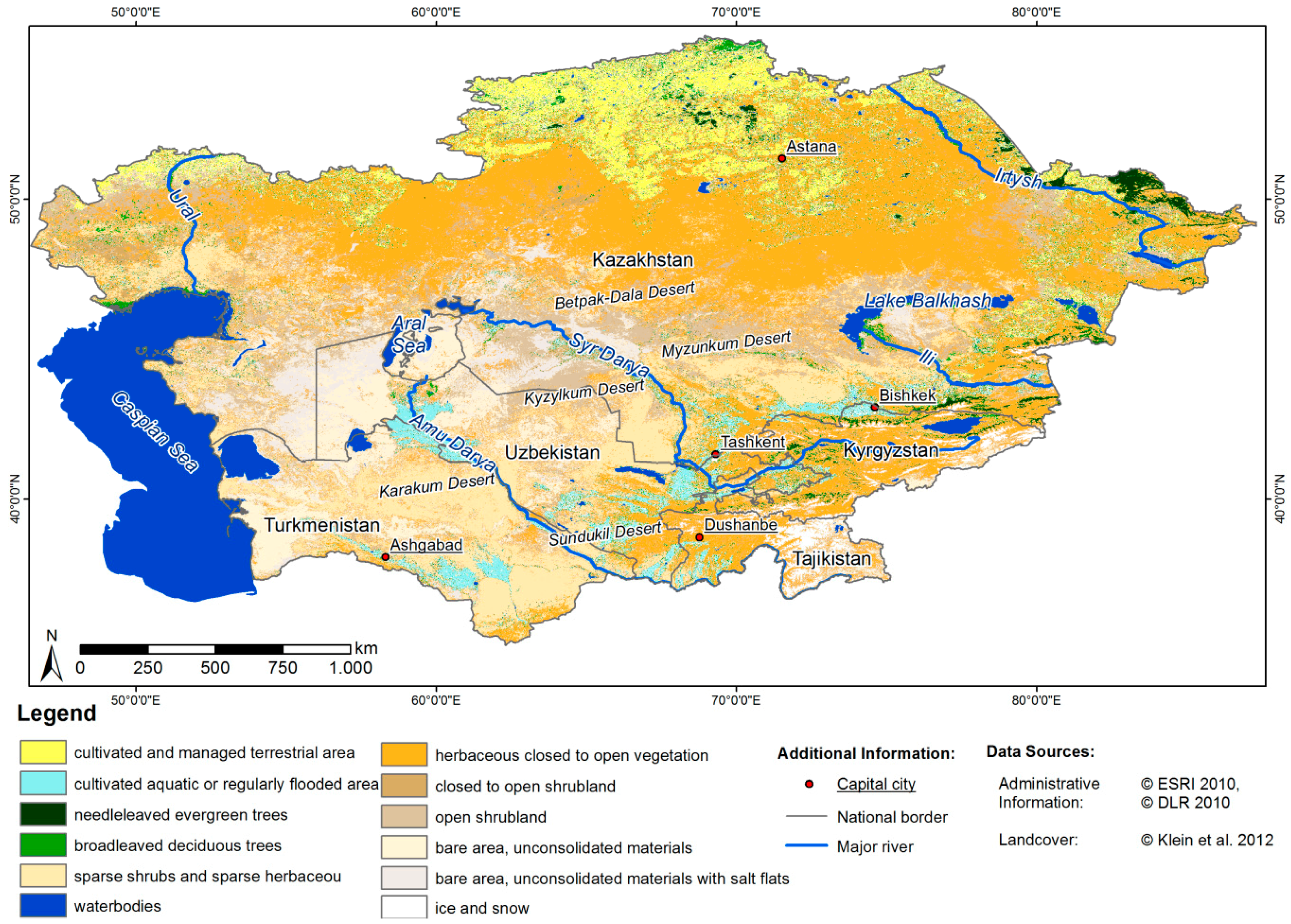
2.1. Study Area
2.2. Datasets
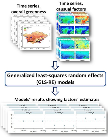
3. Methods
3.1. Data Compilation for Statistical Modelling
3.2. Calculating Seasonality Metrics from NDVI and Climatic Data
3.3. Statistical Modelling
- is the dependent variable where i = entity and t = time,
- represents one independent variable,
- is the coefficient for that X,
- (i = 1….n) is the unknown intercept for each entity (n entity-specific intercepts),
- is the between-entity error,
- is the within-entity error.
4. Results and Discussion
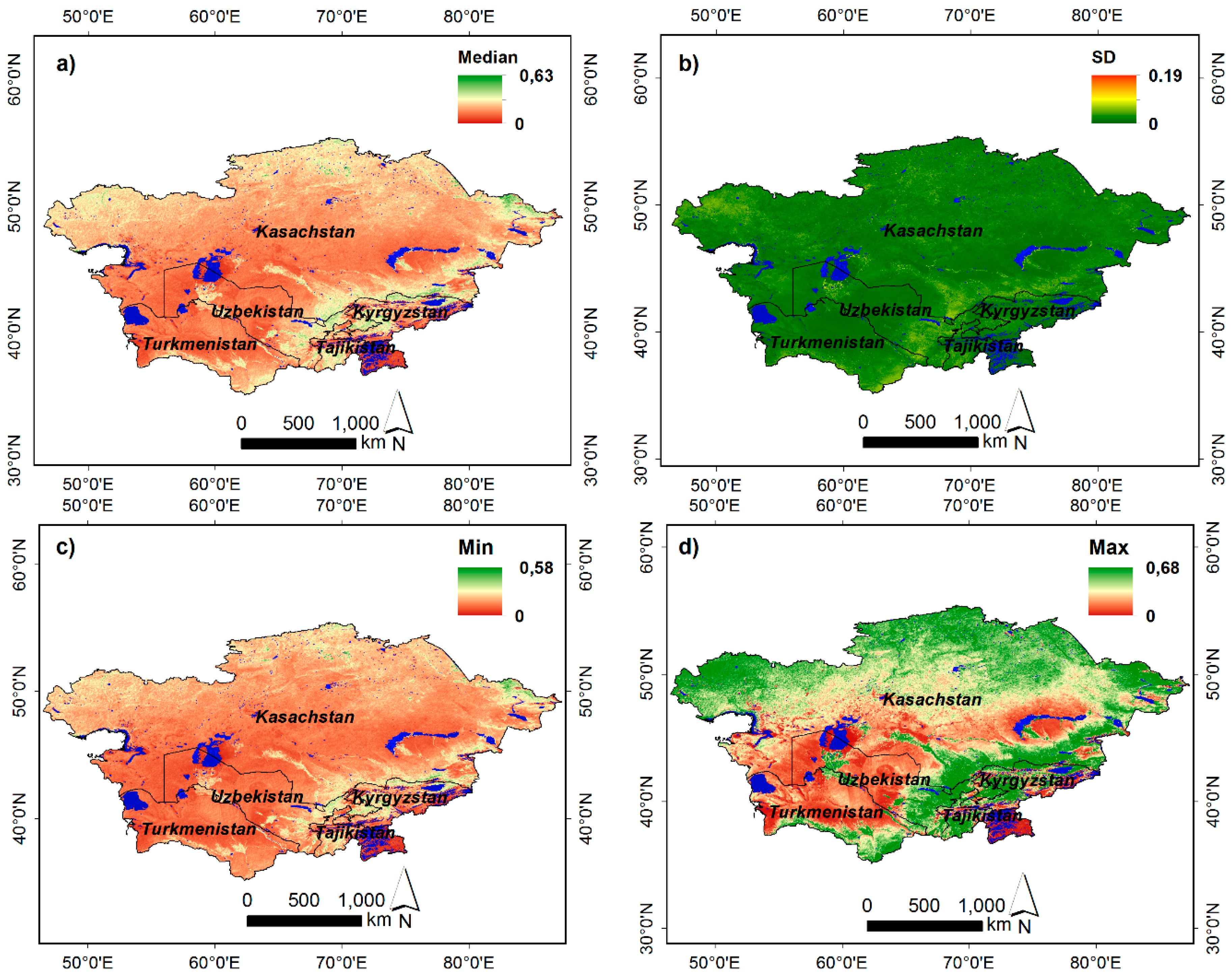
4.1. Distribution of Overall Greenness in Central Asia during 2000–2009
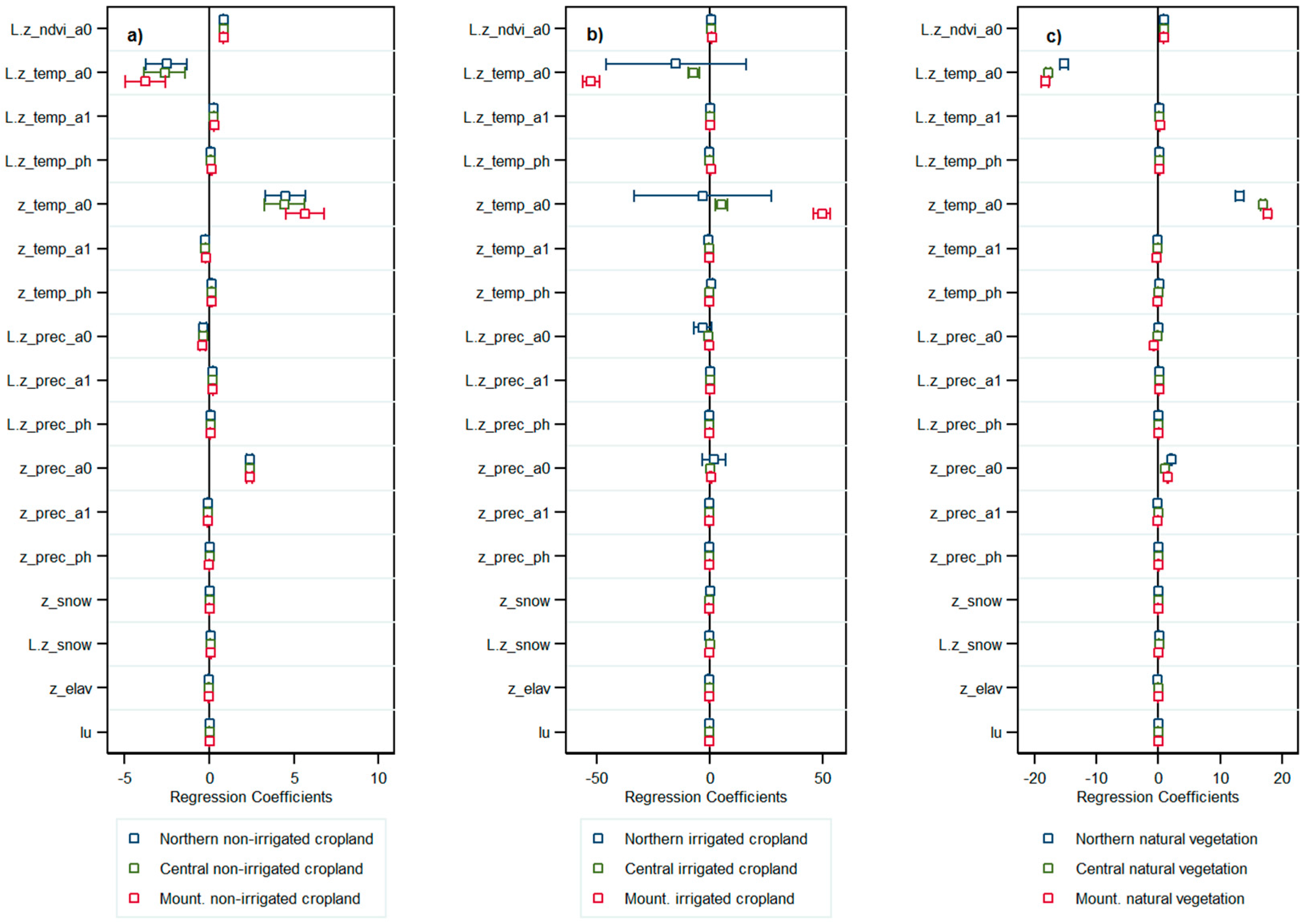
4.2. Factors of Inter-Annual Vegetation Dynamics
4.2.1. Environmental Factors of Inter-Annual Dynamics of Natural Vegetation and Rain Fed Croplands
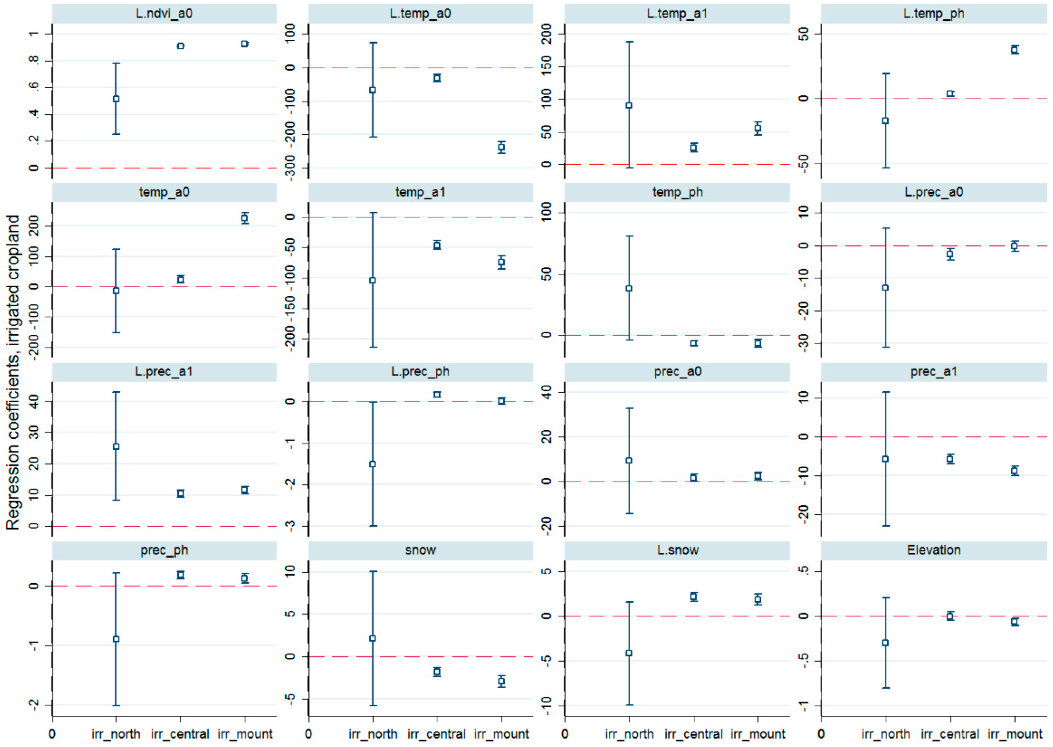
4.2.2. Factors of Inter-Annual Dynamics of Irrigated Croplands
4.2.3. Other Factors of Inter-Annual Vegetation Dynamics of Central Asia
5. Conclusions
Acknowledgments
Author Contributions
Conflicts of Interest
References
- Mueller, L.; Suleimenov, M.; Karimov, A.; Qadir, M.; Saparov, A.; Balgabayev, N.; Helming, K.; Lischeid, G. Land and water resources of Central Asia, their utilisation and ecological status. In Novel Measurement and Assessment Tools for Monitoring and Management of Land and Water Resources in Agricultural Landscapes of Central Asia; Mueller, L., Saparov, A., Lischeid, G., Eds.; Springer International Publishing: Cham, Switzerland, 2014; pp. 3–59. [Google Scholar]
- Karthe, D.; Chalov, S.; Borchardt, D. Water resources and their management in Central Asia in the early twenty first century: Status, challenges and future prospects. Environ. Earth Sci. 2014, 73, 487–499. [Google Scholar] [CrossRef]
- Löw, F.; Fliemann, E.; Abdullaev, I.; Conrad, C.; Lamers, J.P.A. Mapping abandoned agricultural land in Kyzylorda, Kazakhstan using satellite remote sensing. Appl. Geogr. 2015, 62, 377–390. [Google Scholar] [CrossRef]
- Tüshaus, J.; Dubovyk, O.; Khamzina, A.; Menz, G. Comparison of medium spatial resolution ENVISAT-MERIS and Terra-MODIS time series for vegetation decline analysis: A case study in Central Asia. Remote Sens. 2014, 6, 5238–5256. [Google Scholar] [CrossRef]
- Siegfried, T.; Bernauer, T.; Guiennet, R.; Sellars, S.; Robertson, A.; Mankin, J.; Bauer-Gottwein, P.; Yakovlev, A. Will climate change exacerbate water stress in Central Asia? Clim. Chang. 2012, 112, 881–899. [Google Scholar] [CrossRef]
- Fensholt, R.; Proud, S.R. Evaluation of earth observation based global long term vegetation trends—Comparing GIMMS and MODIS global NDVI time series. Remote Sens. Environ. 2012, 119, 131–147. [Google Scholar] [CrossRef]
- Landmann, T.; Dubovyk, O. Spatial analysis of human-induced vegetation productivity decline over Eastern Africa using a decade (2001–2011) of medium resolution MODIS time-series data. Int. J. Appl. Earth Obs. Geoinf. 2014, 33, 76–82. [Google Scholar] [CrossRef]
- Klein, I.; Gessner, U.; Künzer, C. Generation of up to date land cover maps for Central Asia. In Novel Measurement and Assessment Tools for Monitoring and Management of Land and Water Resources in Agricultural Landscapes of Central Asia; Mueller, L., Saparov, A., Lischeid, G., Eds.; Springer International Publishing: Cham, Switzerland, 2014; pp. 329–346. [Google Scholar]
- Bajocco, S.; Angelis, A.; Perini, L.; Ferrara, A.; Salvati, L. The impact of land use/land cover changes on land degradation dynamics: A Mediterranean case study. Environ. Manag. 2012, 49, 980–989. [Google Scholar] [CrossRef] [PubMed]
- Walker, J.J.; de Beurs, K.M.; Henebry, G.M. Land surface phenology along urban to rural gradients in the US Great Plains. Remote Sens. Environ. 2015, 165, 42–52. [Google Scholar] [CrossRef]
- Dubovyk, O.; Landmann, T.; Erasmus, B.F.N.; Tewes, A.; Schellberg, J. Monitoring vegetation dynamics with medium resolution MODIS-EVI time series at sub-regional scale in Southern Africa. Int. J. Appl. Earth Obs. Geoinf. 2015, 38, 175–183. [Google Scholar] [CrossRef]
- Zhou, Y.; Zhang, L.; Fensholt, R.; Wang, K.; Vitkovskaya, I.; Tian, F. Climate contributions to vegetation variations in Central Asian drylands: Pre- and post-USSR collapse. Remote Sens. 2015, 7, 2449–2470. [Google Scholar] [CrossRef]
- Kariyeva, J.; van Leeuwen, W.J.D. Phenological dynamics of irrigated and natural drylands in Central Asia before and after the USSR collapse. Agric. Ecosyst. Environ. 2012, 162, 77–89. [Google Scholar] [CrossRef]
- Gessner, U.; Naeimi, V.; Klein, I.; Kuenzer, C.; Klein, D.; Dech, S. The relationship between precipitation anomalies and satellite-derived vegetation activity in Central Asia. Glob. Planet. Chang. 2013, 110, 74–87. [Google Scholar] [CrossRef]
- Propastin, P.A.; Kappas, M.; Muratova, N.R. Inter-annual changes in vegetation activities and their relationship to temperature and precipitation in Central Asia from 1982 to 2003. J. Environ. Inf. 2008, 12, 75–87. [Google Scholar] [CrossRef]
- De Beurs, K.M.; Henebry, G.M. Land surface phenology, climatic variation, and institutional change: Analyzing agricultural land cover change in Kazakhstan. Remote Sens. Environ. 2004, 89, 497–509. [Google Scholar] [CrossRef]
- Dubovyk, O. Multi-scale Targeting of Land Degradation in Northern Uzbekistan Using Satellite Remote Sensing. Ph.D. Thesis, University of Bonn, Bonn, Germany, 2013. [Google Scholar]
- Dubovyk, O.; Menz, G.; Conrad, C.; Kan, E.; Machwitz, M.; Khamzina, A. Spatio-temporal analyses of cropland degradation in the irrigated lowlands of Uzbekistan using remote-sensing and logistic regression modeling. Environ. Monit. Assess. 2013, 185, 4775–4790. [Google Scholar] [CrossRef] [PubMed]
- De Beurs, K.M.; Henebry, G.M.; Owsley, B.C.; Sokolik, I. Using multiple remote sensing perspectives to identify and attribute land surface dynamics in Central Asia 2001–2013. Remote Sens. Environ. 2015, 170, 48–61. [Google Scholar] [CrossRef]
- Allison, P.D. Fixed Effects Regression Models; SAGE Publications: London, UK, 2009. [Google Scholar]
- Walker, J.J.; de Beurs, K.M.; Wynne, R.H. Dryland vegetation phenology across an elevation gradient in Arizona, USA, investigated with fused MODIS and Landsat data. Remote Sens. Environ. 2014, 144, 85–97. [Google Scholar] [CrossRef]
- Ganguly, S.; Friedl, M.A.; Tan, B.; Zhang, X.; Verma, M. Land surface phenology from MODIS: Characterization of the Collection 5 global land cover dynamics product. Remote Sen. Environ. 2010, 114, 1805–1816. [Google Scholar] [CrossRef]
- Shuai, Y.; Schaaf, C.; Zhang, X.; Strahler, A.; Roy, D.; Morisette, J.; Wang, Z.; Nightingale, J.; Nickeson, J.; Richardson, A.; et al. Daily MODIS 500 m reflectance anisotropy direct broadcast (DB) products for monitoring vegetation phenology dynamics. Int. J. Remote Sens. 2013, 34, 5997–6016. [Google Scholar] [CrossRef]
- Mirzabaev, A.; Goedecke, J.; Dubovyk, O.; Djanibekov, U.; Le, Q.; Aw-Hassan, A. Economics of land degradation in Central Asia. In Economics of Land Degradation and Improvement—A Global Assessment for Sustainable Development; Nkonya, E., Mirzabaev, A., von Braun, J., Eds.; Springer International Publishing: Cham, Switzerland, 2016; pp. 261–290. [Google Scholar]
- Xu, L.; Zhou, H.; Du, L.; Yao, H.; Wang, H. Precipitation trends and variability from 1950 to 2000 in arid lands of Central Asia. J. Arid Land 2015, 7, 514–526. [Google Scholar] [CrossRef]
- Lioubimtseva, E.; Henebry, G.M. Climate and environmental change in arid Central Asia: Impacts, vulnerability, and adaptations. J. Arid Environ. 2009, 73, 963–977. [Google Scholar] [CrossRef]
- Kariyeva, J.; van Leeuwen, W.J.D. Environmental drivers of NDVI-based vegetation phenology in Central Asia. Remote Sens. 2011, 3, 203–246. [Google Scholar] [CrossRef]
- Klein, I.; Gessner, U.; Kuenzer, C. Regional land cover mapping and change detection in Central Asia using MODIS time-series. Appl. Geogr. 2012, 35, 219–234. [Google Scholar] [CrossRef]
- Le, Q.B.; Tamene, L.; Vlek, P.L.G. Multi-pronged assessment of land degradation in West Africa to assess the importance of atmospheric fertilization in masking the processes involved. Glob. Planet. Chang. 2012, 92, 71–81. [Google Scholar] [CrossRef]
- Harris, I.; Jones, P.D.; Osborn, T.J.; Lister, D.H. Updated high-resolution grids of monthly climatic observations—The CRU TS3.10 Dataset. Int. J. Climatol. 2013, 34, 623–642. [Google Scholar] [CrossRef] [Green Version]
- Glantz, M.H. Water, climate, and development issues in the Amu Darya Basin. Mitig. Adapt. Strateg. Glob. Chang. 2005, 10, 23–50. [Google Scholar] [CrossRef]
- Dietz, A.J.; Kuenzer, C.; Dech, S. Global snowpack: A new set of snow cover parameters for studying status and dynamics of the planetary snow cover extent. Remote Sens. Lett. 2015, 6, 844–853. [Google Scholar] [CrossRef]
- Dietz, A.J.; Kuenzer, C.; Conrad, C. Snow-cover variability in Central Asia between 2000 and 2011 derived from improved MODIS daily snow-cover products. Int. J. Remote Sens. 2013, 34, 3879–3902. [Google Scholar] [CrossRef]
- Eastman, R.; Sangermano, F.; Ghimire, B.; Zhu, H.; Chen, H.; Neeti, N.; Cai, Y.; Machado, E.A.; Crema, S.C. Seasonal trend analysis of image time series. Int. J. Remote Sens. 2009, 30, 2721–2726. [Google Scholar] [CrossRef]
- Freedman, D. Statistical Models: Theory and Practice; Cambridge University Press: Cambridge, UK, 2006. [Google Scholar]
- Bradley, B.A.; Jacob, R.W.; Hermance, J.F.; Mustard, J.F. A curve fitting procedure to derive inter-annual phenologies from time series of noisy satellite NDVI data. Remote Sens. Environ. 2007, 106, 137–145. [Google Scholar] [CrossRef]
- Neeti, N.; Rogan, J.; Christman, Z.; Eastman, J.R.; Millones, M.; Schneider, L.; Nickl, E.; Schmook, B.; Turner, B.L.; Ghimire, B. Mapping seasonal trends in vegetation using AVHRR-NDVI time series in the Yucatã¡n Peninsula, Mexico. Remote Sens. Lett. 2012, 3, 433–442. [Google Scholar] [CrossRef]
- De Jong, R.; de Bruin, S.; de Wit, A.; Schaepman, M.E.; Dent, D.L. Analysis of monotonic greening and browning trends from global NDVI time-series. Remote Sens. Environ. 2011, 115, 692–702. [Google Scholar] [CrossRef] [Green Version]
- Kerlinger, F.N. Foundations of Behavioral Research; Holt, Rinehart & Winston: New York, NY, USA, 1964. [Google Scholar]
- Kariyeva, J.; van Leeuwen, W.J.D.; Woodhouse, C.A. Impacts of climate gradients on the vegetation phenology of major land use types in Central Asia (1981–2008). Front. Earth Sci. 2012, 6, 206–225. [Google Scholar] [CrossRef]
- Mirzabaev, A. Climate Volatility and Change in Central Asia: Economic Impacts and Adaptation. Ph.D. Thesis, University of Bonn, Bonn, Germany, 2013. [Google Scholar]
- Aw-Hassan, A.; Korol, V.; Nishanov, N.; Djanibekov, U.; Dubovyk, O.; Mirzabaev, A. Economics of land degradation and improvement in Uzbekistan. In Economics of Land Degradation and Improvement—A Global Assessment for Sustainable Development; Nkonya, E., Mirzabaev, A., von Braun, J., Eds.; Springer International Publishing: Cham, Switzerland, 2016; pp. 651–682. [Google Scholar]
- Dubovyk, O.; Landmann, T.; Erasmus, B.; Thonfeld, F.; Schellberg, J.; Menz, G. Observing vegetation dynamics at medium spatial scale: Lessons from Africa and Asia. In Proceedings of the 2015 IEEE International Geoscience and Remote Sensing Symposium (IGARSS), Milan, Italy, 26–31 July 2015; pp. 3969–3972.
- Lu, L.; Guo, H.; Kuenzer, C.; Klein, I.; Zhang, L.; Li, X. Analyzing phenological changes with remote sensing data in Central Asia. IOP Conf. Ser.: Earth Environ. Sci. 2014, 17, 012005. [Google Scholar] [CrossRef]
- Dukhovny, V.A.; de Schutter, J. Water in Central Asia: Past, Present, Future; CRC Press: London, UK, 2011. [Google Scholar]
- Shigaeva, J.; Kollmair, M.; Niederer, P.; Maselli, D. Livelihoods in transition: Changing land use strategies and ecological implications in a post-Soviet setting (Kyrgyzstan). Cent. Asian Surv. 2007, 26, 389–406. [Google Scholar] [CrossRef]
- Bucknall, J.; Klytchnikova, I.; Lampietti, J.; Lundell, M.; Scatasta, M.; Thurman, M. Irrigation in Central Asia: Social, Economic and Environmental Considerations; World Bank: Washington, DC, USA, 2003. [Google Scholar]
- Kraemer, R.; Prishchepov, A.V.; Müller, D.; Kuemmerle, T.; Radeloff, V.C.; Dara, A.; Terekhov, A.; Frühauf, M. Long-term agricultural land-cover change and potential for cropland expansion in the former Virgin Lands area of Kazakhstan. Environ. Res. Lett. 2015, 10, 054012. [Google Scholar] [CrossRef]
- Meyfroidt, P.; Schierhorn, F.; Prishchepov, A.V.; Müller, D.; Kuemmerle, T. Drivers, constraints and trade-offs associated with recultivating abandoned cropland in Russia, Ukraine and Kazakhstan. Glob. Environ. Chang. 2016, 37, 1–15. [Google Scholar] [CrossRef]
- Djanibekov, N.; Bobojonov, I.; Lamers, J.A. Farm reform in Uzbekistan. In Cotton, Water, Salts and Soums; Martius, C., Rudenko, I., Lamers, J.P.A., Vlek, P.L.G., Eds.; Springer Netherlands: Dordrecht, The Netherlands, 2012; pp. 95–112. [Google Scholar]


| Variable | Description | Time Step | Data Source |
|---|---|---|---|
| L.ndvi_a0 | Lagged overall greenness | Yearly | MOD13Q1 |
| temp_a0 | Overall temperature | Yearly | CRU TS3.10 |
| temp_a1 | Peak temperature | Yearly | |
| temp_ph | Timing of peak temperature | Yearly | |
| L.temp_a0 | Lagged overall temperature | Yearly | |
| L.temp_a1 | Lagged peak temperature | Yearly | |
| L.temp_ph | Lagged timing of peak temperature | Yearly | |
| prec_a0 | Overall precipitation | Yearly | |
| prec_a1 | Peak precipitation | Yearly | |
| prec_ph | Timing of peak precipitation | Yearly | |
| L.prec_a0 | Lagged overall precipitation | Yearly | |
| L.prec_a1 | Lagged peak precipitation | Yearly | |
| L.prec_ph | Lagged timing of peak precipitation | Yearly | |
| snow | Stop of the snow cover season | Yearly | MOD10A1, MYD10A1 |
| L.snow | Lagged stop of the snow cover season | Yearly | |
| elav | Slope | Time invariant | SRTM |
| LU | Land use land cover | Year 2009 | MYD13Q1, MYD09Q1 |
| Irrigated | Non-irrigated | Natural Vegetation | |||||||
|---|---|---|---|---|---|---|---|---|---|
| Variable | N. | C. | M. | N. | C. | M. | N. | C. | M. |
| L.ndvi_a0 | 29 | 87 | 84 | 72 | 72 | 73 | 74 | 78 | 83 |
| L.temp_a0 | 2 | 0 | 10 | 0 | 0 | 0 | 2 | 4 | 3 |
| L.temp_a1 | 8 | 1 | 2 | 5 | 5 | 6 | 4 | 2 | 7 |
| L.temp_ph | 2 | 0 | 7 | 0 | 0 | 0 | 1 | 2 | 1 |
| temp_a0 | 0 | 0 | 9 | 0 | 0 | 0 | 2 | 3 | 3 |
| temp_a1 | 8 | 2 | 3 | 3 | 3 | 3 | 2 | 2 | 6 |
| temp_ph | 8 | 1 | 0 | 0 | 0 | 0 | 0 | 0 | 1 |
| L.prec_a0 | 5 | 0 | 0 | 0 | 0 | 0 | 0 | 0 | 0 |
| L.prec_a1 | 18 | 3 | 6 | 6 | 6 | 6 | 4 | 5 | 4 |
| L.prec_ph | 10 | 0 | 0 | 1 | 1 | 0 | 1 | 0 | 0 |
| prec_a0 | 2 | 0 | 0 | 2 | 2 | 2 | 2 | 1 | 1 |
| prec_a1 | 1 | 1 | 3 | 1 | 1 | 1 | 1 | 1 | 2 |
| prec_ph | 6 | 0 | 0 | 0 | 0 | 0 | 0 | 0 | 0 |
| snow | 1 | 1 | 1 | 0 | 0 | 0 | 0 | 0 | 0 |
| L.snow | 5 | 1 | 0 | 0 | 0 | 0 | 1 | 1 | 0 |
| LULC | 0 | 0 | 4 | 0 | 1 | 1 | 0 | 0 | 0 |
| elav | 4 | 0 | 0 | 0 | 0 | 0 | 1 | 0 | 0 |
© 2016 by the authors; licensee MDPI, Basel, Switzerland. This article is an open access article distributed under the terms and conditions of the Creative Commons Attribution (CC-BY) license (http://creativecommons.org/licenses/by/4.0/).
Share and Cite
Dubovyk, O.; Landmann, T.; Dietz, A.; Menz, G. Quantifying the Impacts of Environmental Factors on Vegetation Dynamics over Climatic and Management Gradients of Central Asia. Remote Sens. 2016, 8, 600. https://doi.org/10.3390/rs8070600
Dubovyk O, Landmann T, Dietz A, Menz G. Quantifying the Impacts of Environmental Factors on Vegetation Dynamics over Climatic and Management Gradients of Central Asia. Remote Sensing. 2016; 8(7):600. https://doi.org/10.3390/rs8070600
Chicago/Turabian StyleDubovyk, Olena, Tobias Landmann, Andreas Dietz, and Gunter Menz. 2016. "Quantifying the Impacts of Environmental Factors on Vegetation Dynamics over Climatic and Management Gradients of Central Asia" Remote Sensing 8, no. 7: 600. https://doi.org/10.3390/rs8070600