
Sixteen Years of Agricultural Drought Assessment of the BioBío Region in Chile Using a 250 m Resolution Vegetation Condition Index (VCI)

 ,
,  ,
,
Abstract
:
1. Introduction
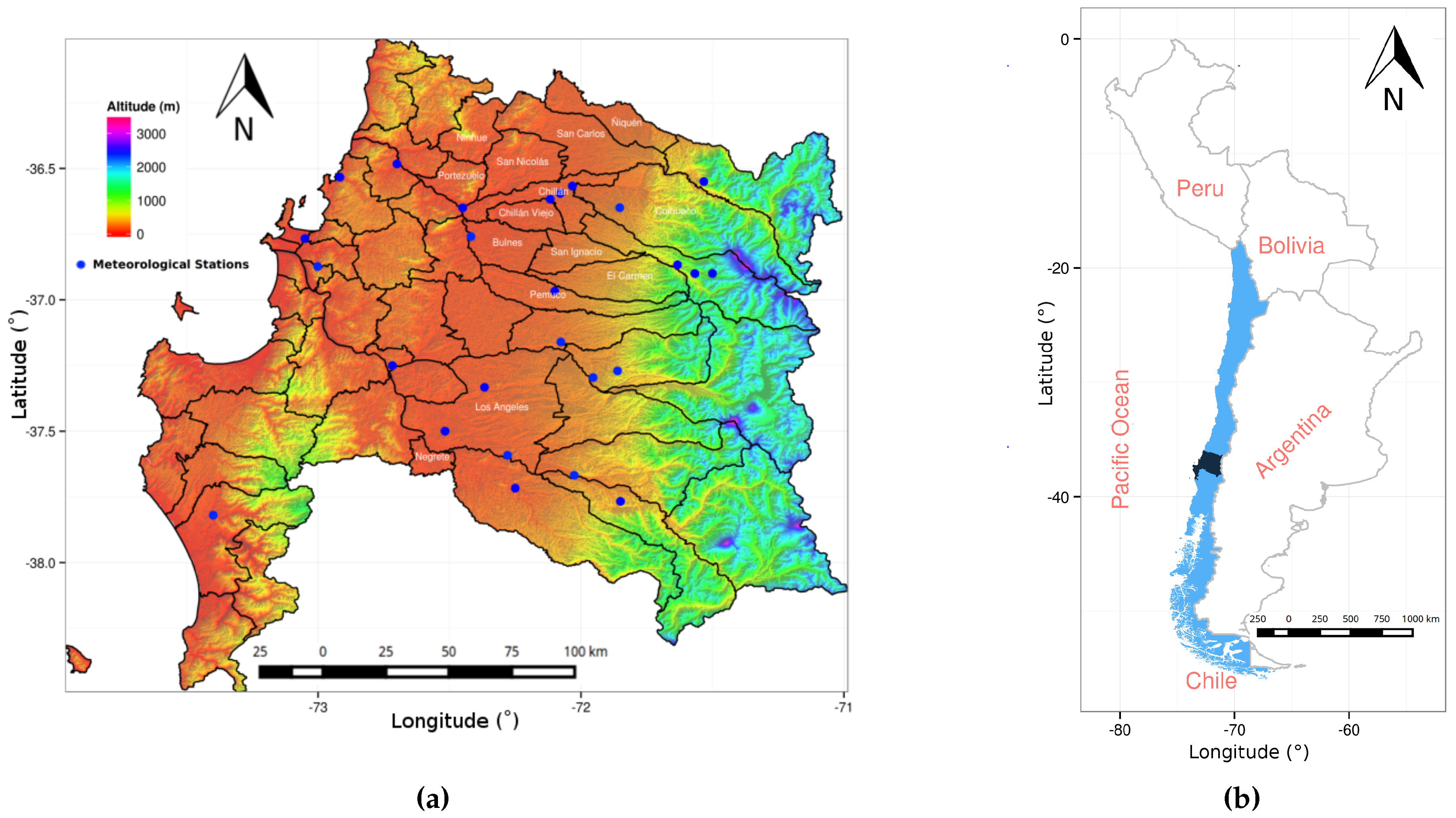
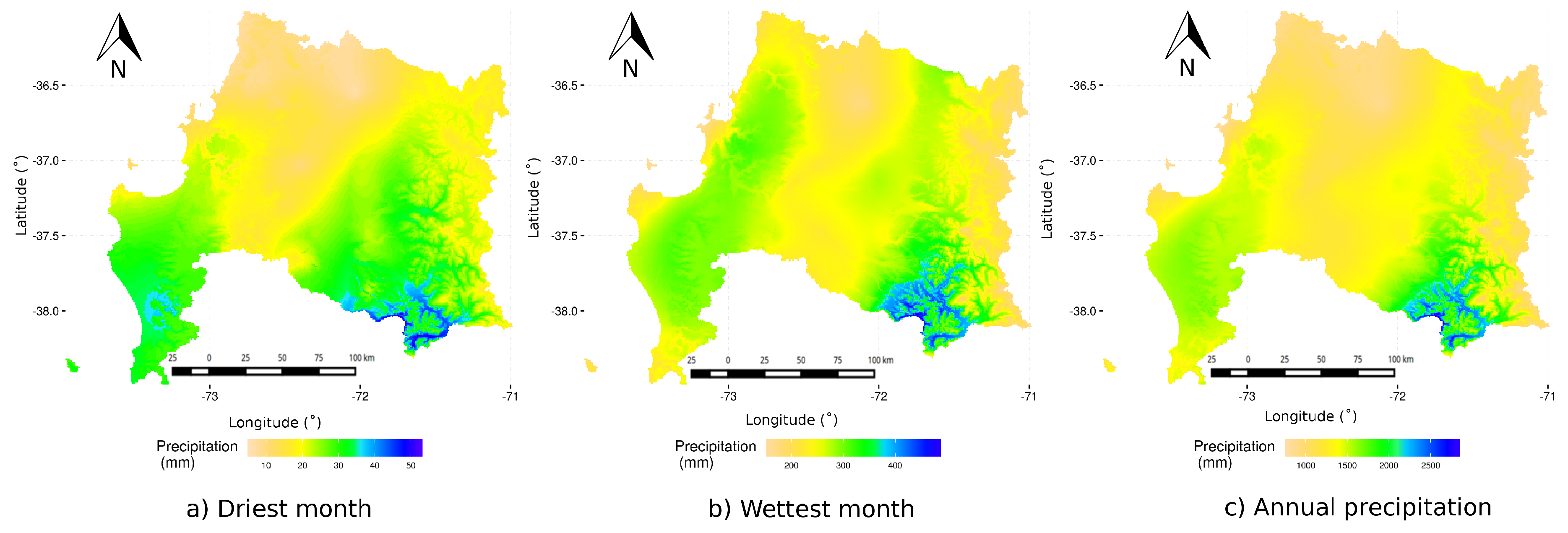
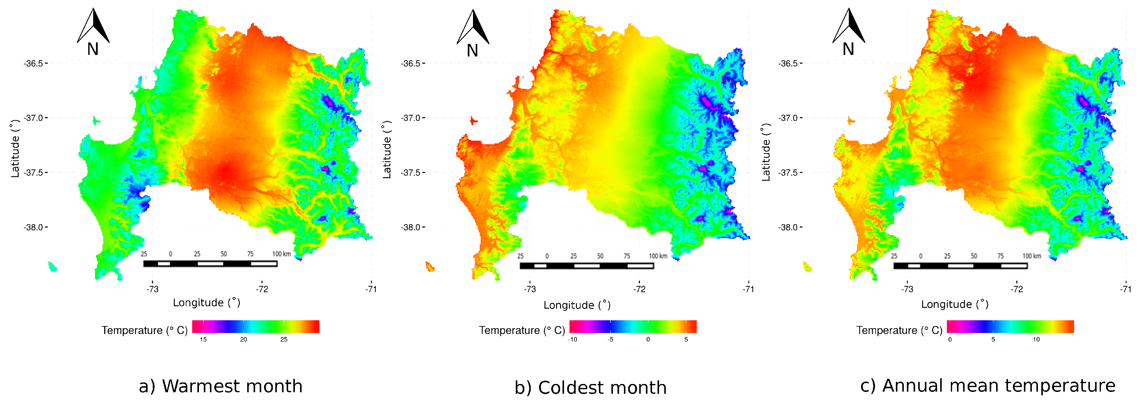
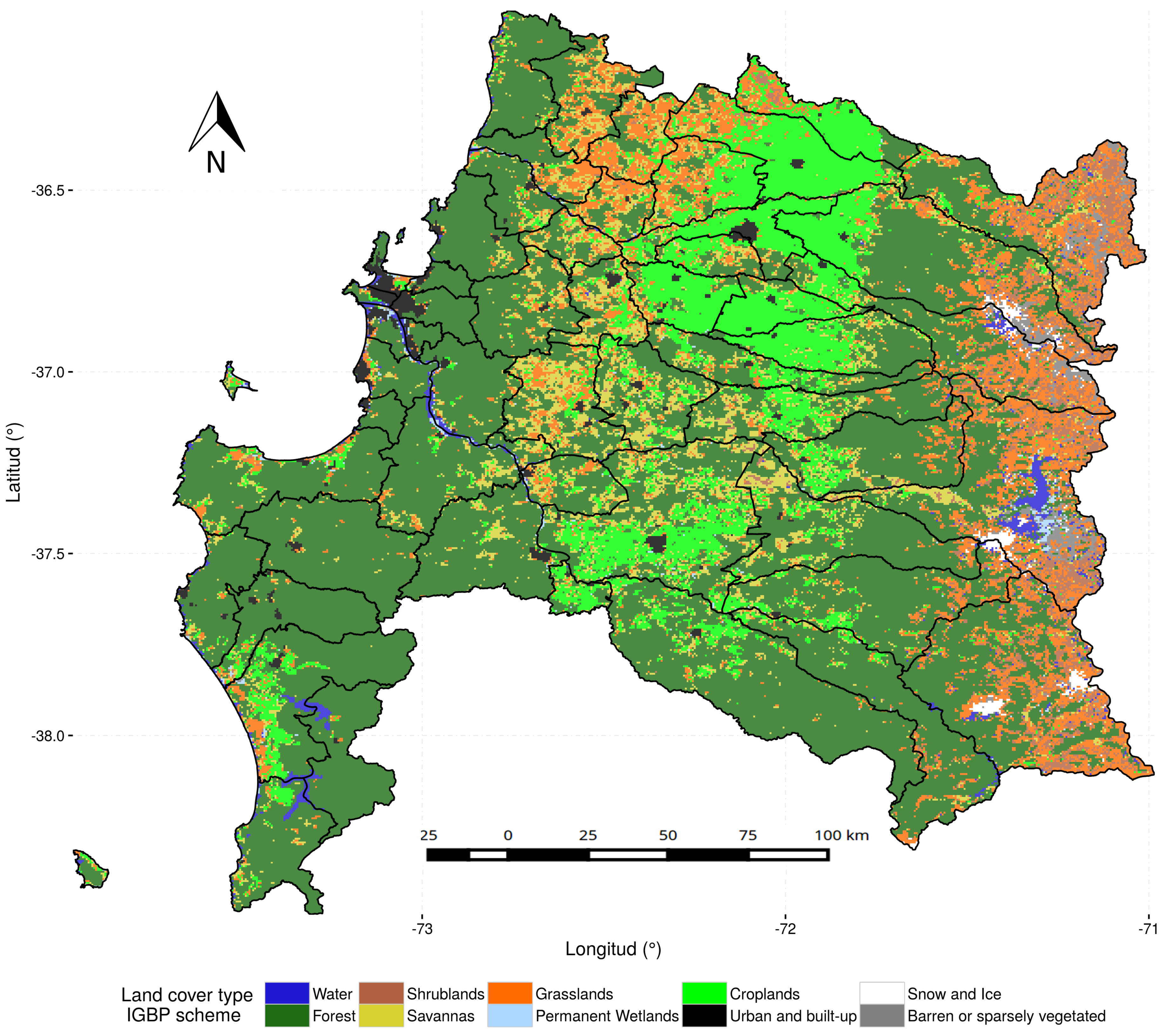
2. Study Area
3. Data
4. Methods
4.1. Procedure for Calculating VCI in Cropland Areas
4.2. Cropland Mask
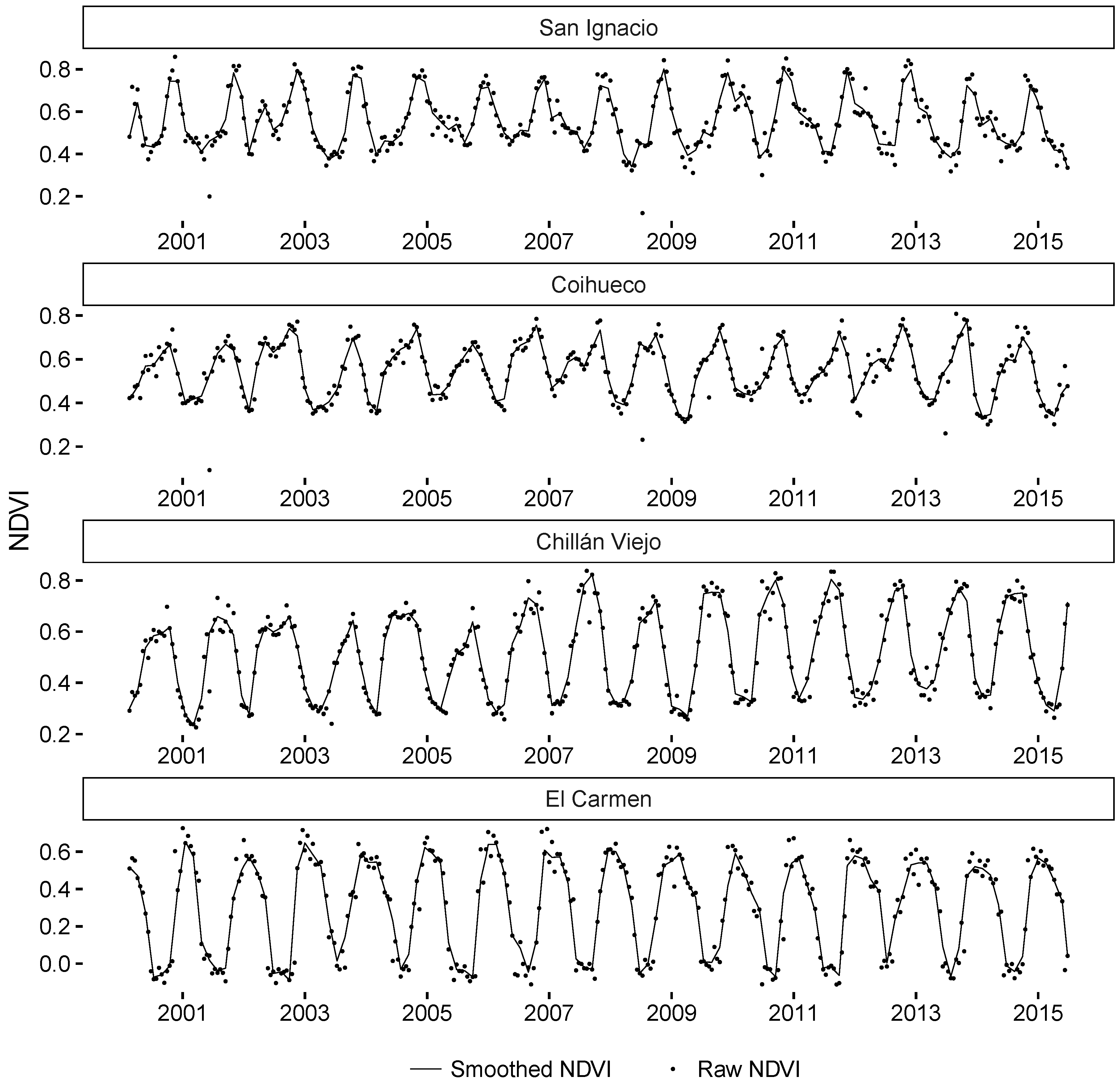
4.3. Vegetation Condition Index (VCI)
4.4. Standardized Precipitation Index (SPI)
4.5. Correlation between VCI and SPI
5. Results and Discussion
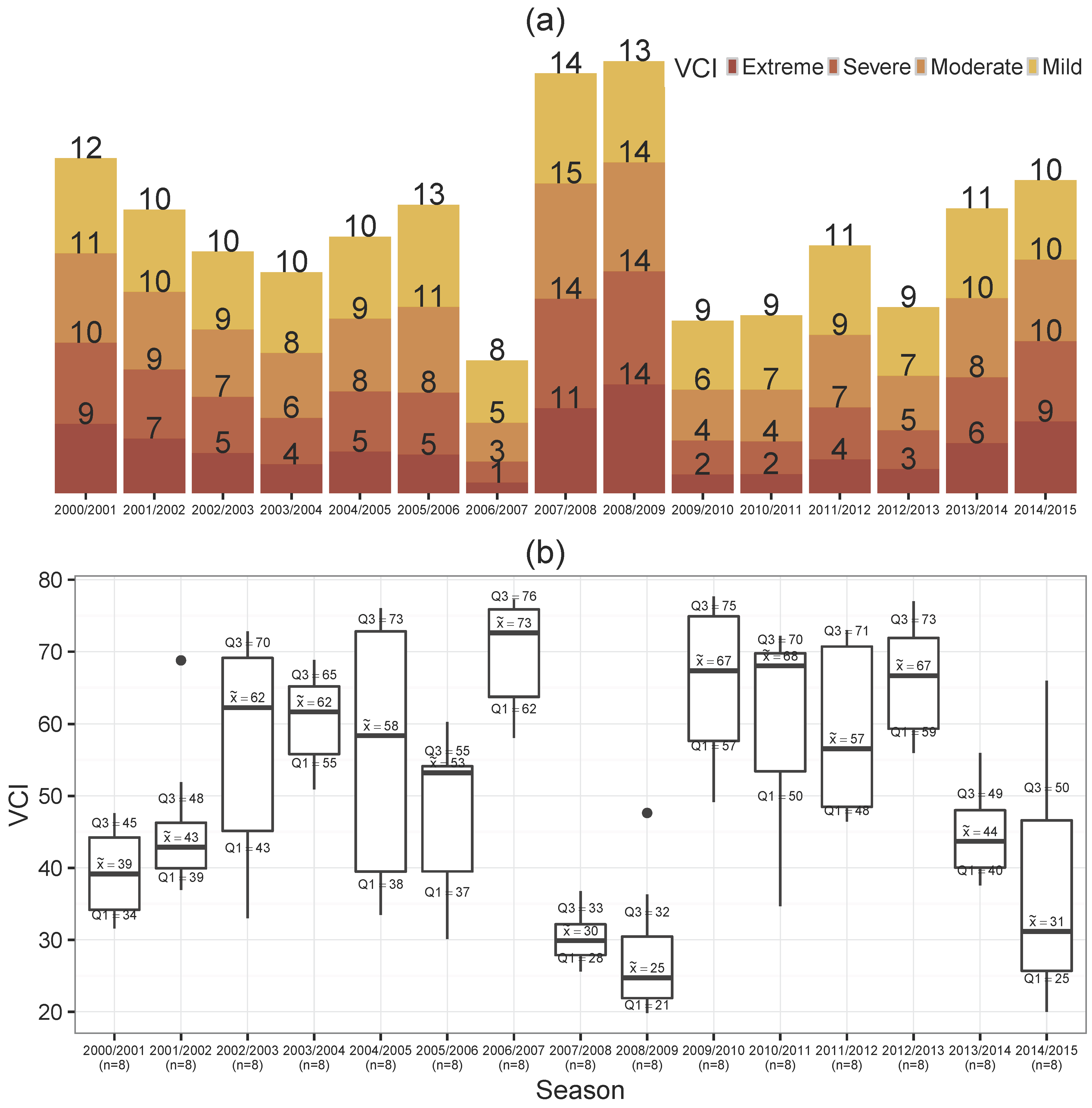
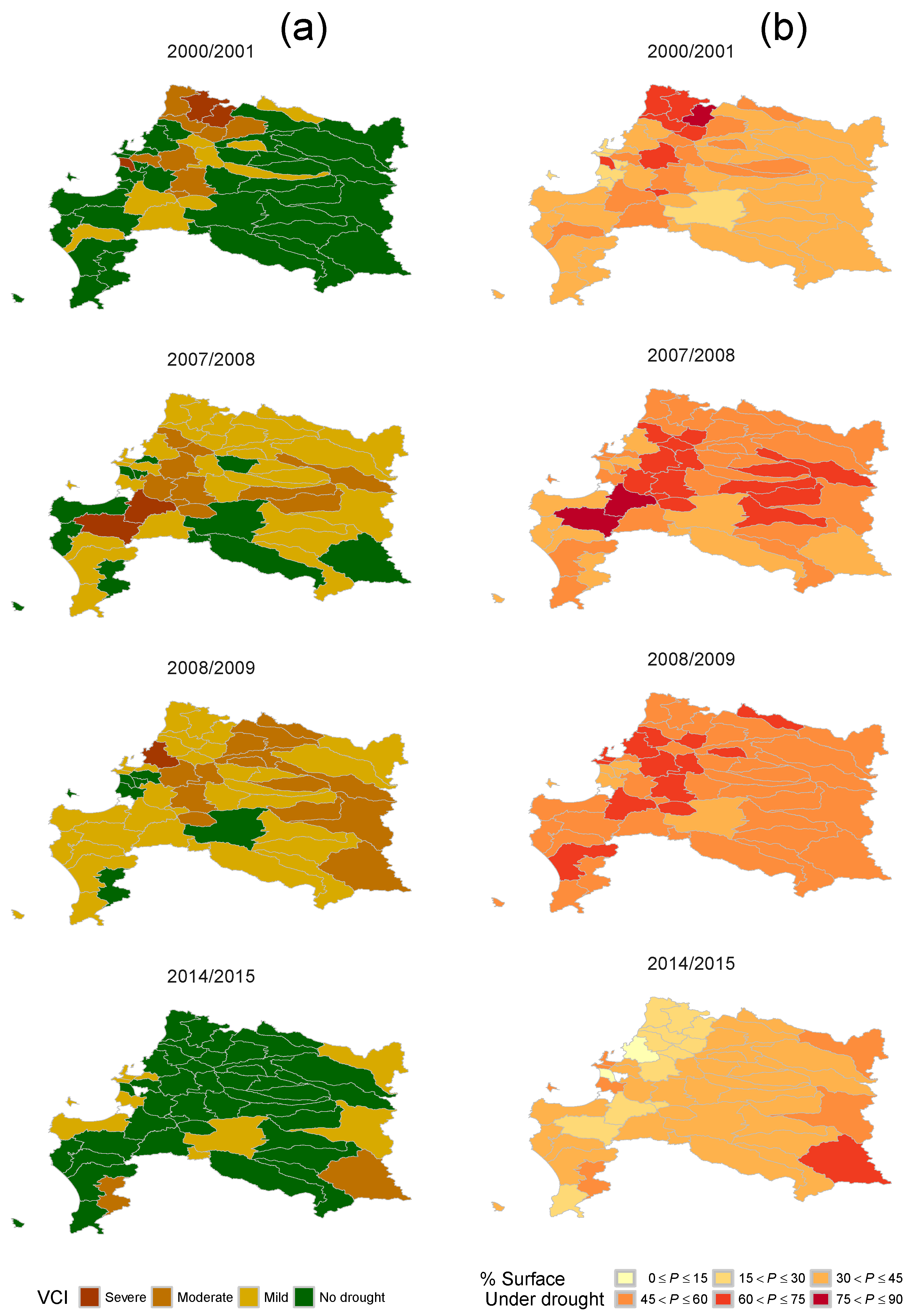
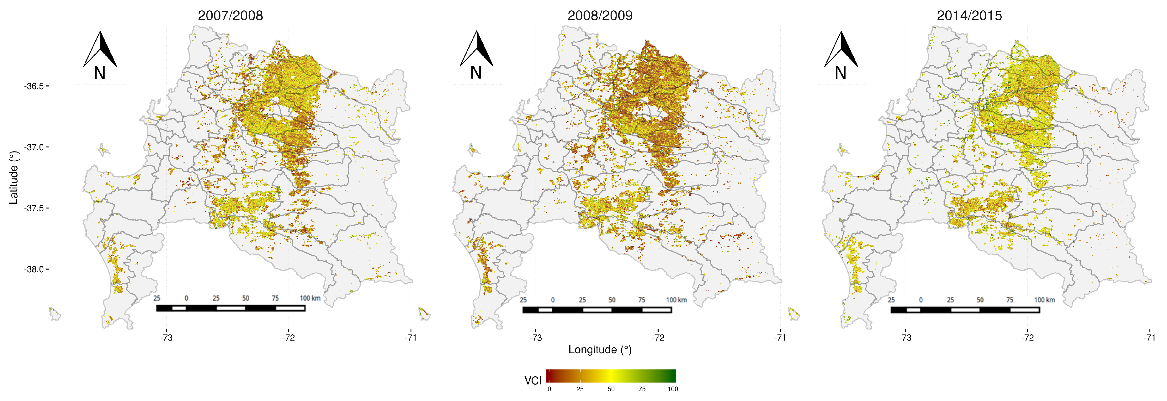
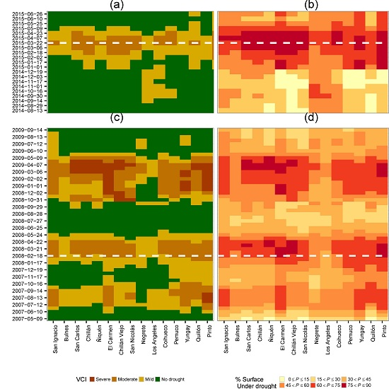
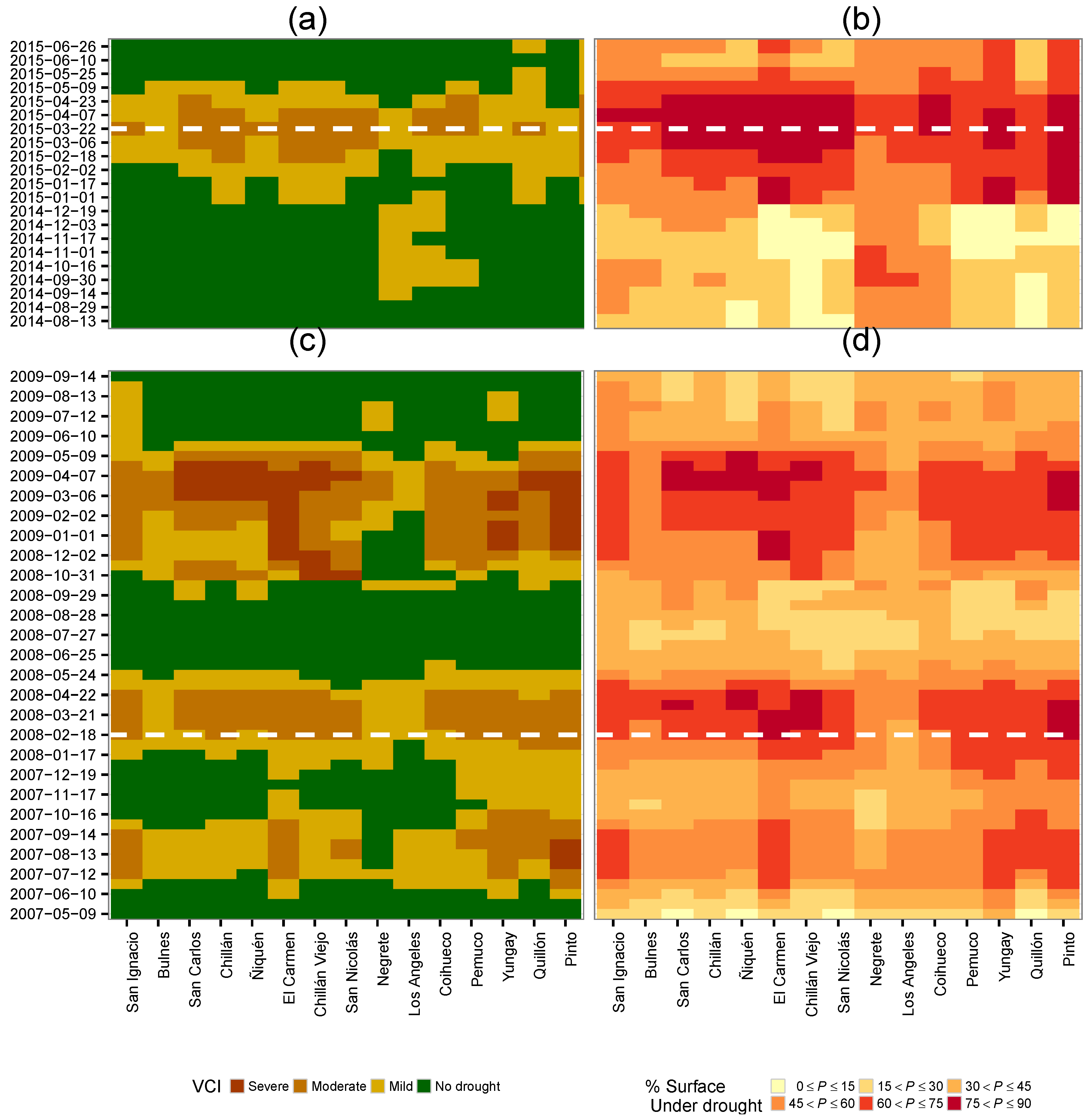
5.1. Spatio-Temporal Variation of VCI and Comparison with Drought Declaration
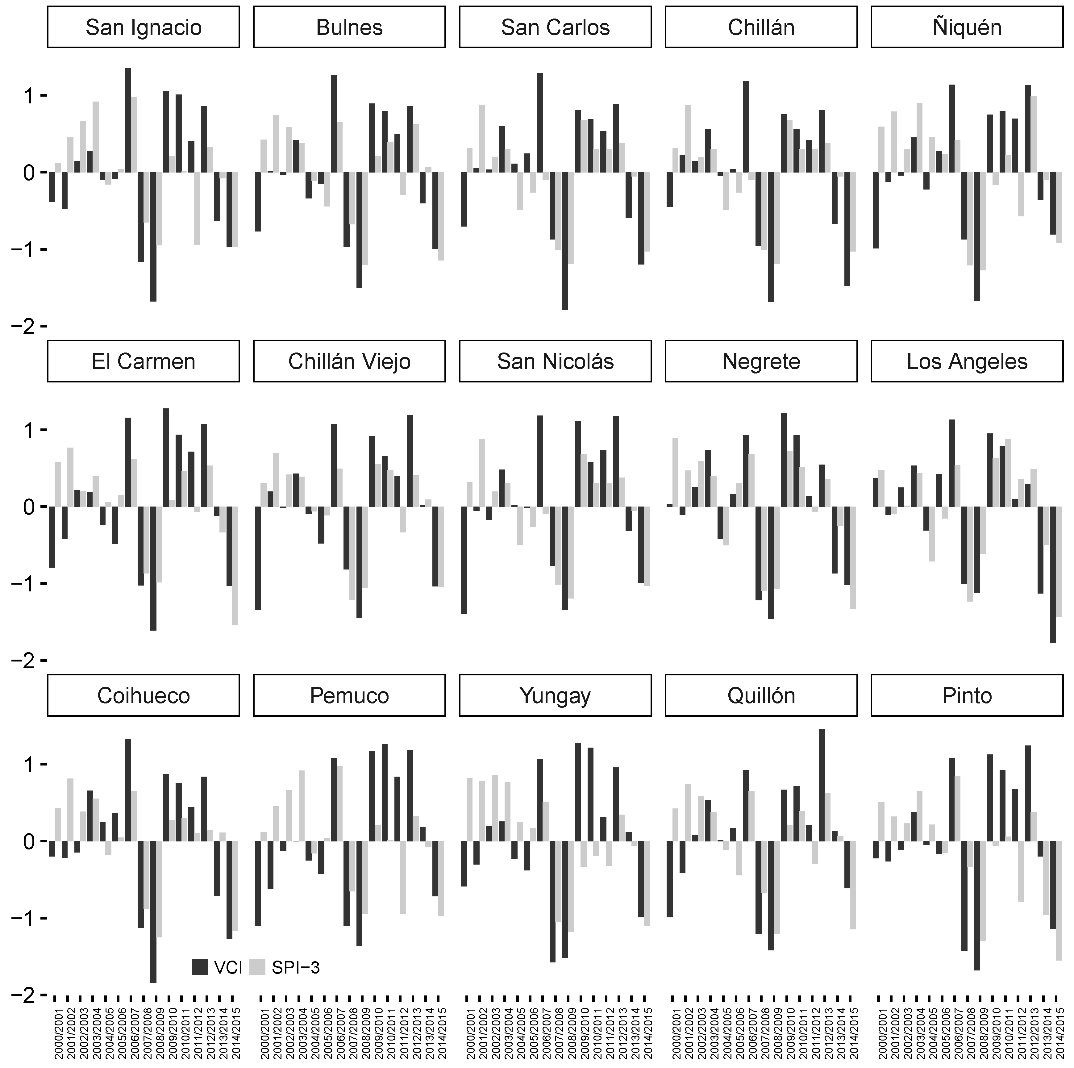
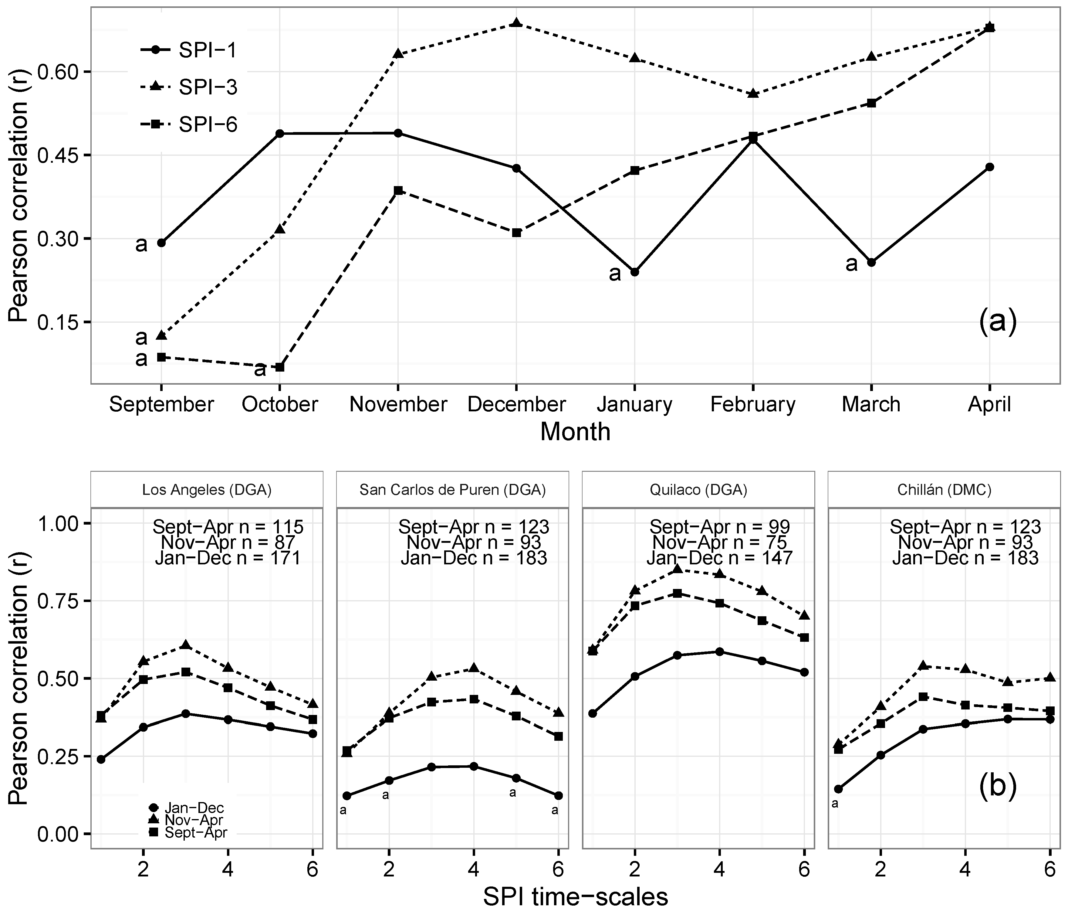
5.2. Correlation VCI vs. SPI
6. Conclusions
Acknowledgments
Author Contributions
Conflicts of Interest
References
- Dore, M.H. Climate change and changes in global precipitation patterns: What do we know? Environ. Int. 2005, 31, 1167–1181. [Google Scholar] [CrossRef] [PubMed]
- IPCC. Climate Change 2013: The Physical Science Basis. Contribution of Working Group I to the Fifth Assessment Report of the Intergovernmental Panel on Climate Change; Cambridge University Press: Cambridge, UK; New York, NY, USA, 2013; p. 1535. [Google Scholar]
- Wilhite, D.A.; Glantz, M.H. Understanding: The Drought Phenomenon: The Role of Definitions. Water Int. 1985, 10, 111–120. [Google Scholar] [CrossRef]
- Niemeyer, S. New drought indices. Opt. Méd. 2008, 267–274. [Google Scholar]
- Amin, Z.; Rehan, S.; Bahman, N.; Faisal, K. A review of drought indices. Environ. Rev. 2011, 19, 333–349. [Google Scholar]
- McKee, T.B.; Doesken, N.J.; Kleist, J. The relationship of drought frecuency and duration to time scales. In Proceedings of the International 8th Conference on Applied Climatology, Anaheim, CA, USA, 17–22 January 1993; pp. 179–184.
- Mishra, A.K.; Singh, V.P. A review of drought concepts. J. Hydrol. 2010, 391, 202–216. [Google Scholar] [CrossRef]
- Vicente-Serrano, S.M.; Beguería, S.; López-Moreno, J.I. A multiscalar drought index sensitive to global warming: The standardized precipitation evapotranspiration index. J. Clim. 2010, 23, 1696–1718. [Google Scholar] [CrossRef]
- Palmer, W.C. Meteorological Drought; Research Paper No. 45; US Department of Commerce, Weather Bureau: Washington, DC, USA, 1965.
- Alley, W.M. The palmer drought severity index: Limitations and assumptions. J. Clim. Appl. Meteor. 1984, 23, 1100–1109. [Google Scholar] [CrossRef]
- Palmer, W.C. Keeping track of crop moisture conditions, nationwide: The new crop moisture index. Weatherwise 1968, 21, 156–161. [Google Scholar] [CrossRef]
- Shafer, B.A.; Dezman, L.E. Development of a Surface Water Supply Index (SWSI) to Assess the Severity of Drought Conditions in Snowpack Runoff Areas. In Proceedings of the Western Snow Conference, Fort Collins, CO, USA, 19–23 April 1982; pp. 164–175.
- Vicente-Serrano, S.M.; López-Moreno, J.I.; Beguería, S.; Lorenzo-Lacruz, J.; Azorin-Molina, C.; Morán-Tejeda, E. Accurate computation of a streamflow drought index. J. Hydrol. Eng. 2012, 17, 318–332. [Google Scholar] [CrossRef]
- Caccamo, G.; Chisholm, L.; Bradstock, R.; Puotinen, M. Assessing the sensitivity of MODIS to monitor drought in high biomass ecosystems. Remote. Sens. Environ. 2011, 115, 2626–2639. [Google Scholar] [CrossRef]
- Wu, J.; Zhou, L.; Liu, M.; Zhang, J.; Leng, S.; Diao, C. Establishing and assessing the Integrated Surface Drought Index (ISDI) for agricultural drought monitoring in mid-eastern China. Int. J. Appl. Earth Obs. Geoinf. 2013, 23, 397–410. [Google Scholar] [CrossRef]
- Rojas, O.; Vrieling, A.; Rembold, F. Assessing drought probability for agricultural areas in Africa with coarse resolution remote sensing imagery. Remote. Sens. Environ. 2011, 115, 343–352. [Google Scholar] [CrossRef]
- Rhee, J.; Im, J.; Carbone, G.J. Monitoring agricultural drought for arid and humid regions using multi-sensor remote sensing data. Remote. Sens. Environ. 2010, 114, 2875–2887. [Google Scholar] [CrossRef]
- Logan, K.; Brunsell, N.; Jones, A.; Feddema, J. Assessing spatiotemporal variability of drought in the U.S. central plains. J. Arid. Environ. 2010, 74, 247–255. [Google Scholar] [CrossRef]
- Kogan, F.N. Application of vegetation index and brightness temperature for drought detection. Adv. Space Res. 1995, 15, 91–100. [Google Scholar] [CrossRef]
- Tonini, F.; Lasinio, G.J.; Hochmair, H.H. Mapping return levels of absolute NDVI variations for the assessment of drought risk in Ethiopia. Int. J. Appl. Earth Obs. Geoinf. 2012, 18, 564–572. [Google Scholar] [CrossRef]
- Skakun, S.; Kussul, N.; Shelestov, A.; Kussul, O. The use of satellite data for agriculture drought risk quantification in Ukraine. Geomat. Nat. Haz. Risk 2016, 7, 901–917. [Google Scholar] [CrossRef]
- Rembold, F.; Atzberger, C.; Savin, I.; Rojas, O. Using low resolution satellite imagery for yield prediction and yield anomaly detection. Remote Sens. 2013, 5, 1704–1733. [Google Scholar] [CrossRef] [Green Version]
- Rembold, F.; Meroni, M.; Rojas, O.; Atzberger, C.; Ham, F.; Fillol, E. Chapter 14. Agricultural Drought Monitoring Using Space-Derived Vegetation and Biophysical Products: A Global Perspective; CRC Press: Boca Raton, FL, USA, 2015; pp. 349–365. [Google Scholar]
- Kogan, F.N. Global drought watch from space. Bull. Am. Metor. Soc. 1997, 78, 621–636. [Google Scholar] [CrossRef]
- Kogan, F.N. Droughts of the late 1980s in the United States as derived from NOAA polar-orbiting satellite data. Bull. Am. Metor. Soc. 1995, 76, 655–668. [Google Scholar] [CrossRef]
- Zhang, A.; Jia, G. Monitoring meteorological drought in semiarid regions using multi-sensor microwave remote sensing data. Remote. Sens. Environ. 2013, 134, 12–23. [Google Scholar] [CrossRef]
- Gebrehiwot, T.; van der Veen, A.; Maathuis, B. Spatial and temporal assessment of drought in the northern highlands of Ethiopia. Int. J. Appl. Earth Obs. Geoinf. 2011, 13, 309–321. [Google Scholar] [CrossRef]
- Singh, R.P.; Roy, S.; Kogan, F. Vegetation and temperature condition indices from NOAA AVHRR data for drought monitoring over India. Int. J. Remote Sens. 2003, 24, 4393–4402. [Google Scholar] [CrossRef]
- Seiler, R.; Kogan, F.; Sullivan, J. AVHRR-based vegetation and temperature condition indices for drought detection in Argentina. Adv. Space Res. 1998, 21, 481–484. [Google Scholar] [CrossRef]
- Unganai, L.S.; Kogan, F.N. Drought Monitoring and Corn Yield Estimation in Southern Africa from AVHRR Data. Remote. Sens. Environ. 1998, 63, 219–232. [Google Scholar] [CrossRef]
- Sandholt, I.; Rasmussen, K.; Andersen, J. A simple interpretation of the surface temperature/vegetation index space for assessment of surface moisture status. Remote. Sens. Environ. 2002, 79, 213–224. [Google Scholar] [CrossRef]
- Wang, P.X.; Li, X.W.; Gong, J.Y.; Song, C. Vegetation temperature condition index and its application for drought monitoring. In Proceeding of the IEEE 2001 International Geoscience and Remote Sensing Symposium, IGARSS ’01, Sydney, NSW, Australia, 9–13 July 2001; pp. 141–143.
- Wan, Z.; Wang, P.; Li, X. Using MODIS land surface temperature and normalized difference vegetation index products for monitoring drought in the southern Great Plains, USA. Int. J. Remote Sens. 2004, 25, 61–72. [Google Scholar] [CrossRef]
- Vicente-Serrano, S.M. Evaluating the impact of drought using remote sensing in a mediterranean, semi-arid region. Nat. Hazards 2007, 40, 173–208. [Google Scholar] [CrossRef]
- Zhang, F.; Zhang, L.W.; Wang, X.Z.; Hung, J.F. Detecting agro-droughts in southwest of China using MODIS satellite data. J. Integr. Agric. 2013, 12, 159–168. [Google Scholar] [CrossRef]
- Du, L.; Tian, Q.; Yu, T.; Meng, Q.; Jancso, T.; Udvardy, P.; Huang, Y. A comprehensive drought monitoring method integrating MODIS and TRMM data. Int. J. Appl. Earth Obs. Geoinf. 2013, 23, 245–253. [Google Scholar] [CrossRef]
- Mu, Q.; Zhao, M.; Kimball, J.S.; McDowell, N.G.; Running, S.W. A remotely sensed global terrestrial drought severity index. Bull. Am. Meteor. Soc. 2013, 94, 83–98. [Google Scholar] [CrossRef]
- Enenkel, M.; Steiner, C.; Mistelbauer, T.; Dorigo, W.; Wagner, W.; See, L.; Atzberger, C.; Schneider, S.; Rogenhofer, E. A combined satellite-derived drought indicator to support humanitarian aid organizations. Remote Sens. 2016, 8, 340. [Google Scholar] [CrossRef]
- Kogan, F.N. Remote sensing of weather impacts on vegetation in non-homogeneous areas. Int. J. Remote Sens. 1990, 11, 1405–1419. [Google Scholar] [CrossRef]
- Hird, J.N.; McDermid, G.J. Noise reduction of NDVI time series: An empirical comparison of selected techniques. Remote. Sens. Environ. 2009, 113, 248–258. [Google Scholar] [CrossRef]
- Klisch, A.; Atzberger, C. Operational drought monitoring in Kenya using MODIS NDVI time series. Remote Sens. 2016, 8, 267. [Google Scholar] [CrossRef]
- Julien, Y.; Sobrino, J.A. Comparison of cloud-reconstruction methods for time series of composite NDVI data. Remote. Sens. Environ. 2010, 114, 618–625. [Google Scholar] [CrossRef]
- Atkinson, P.M.; Jeganathan, C.; Dash, J.; Atzberger, C. Inter-comparison of four models for smoothing satellite sensor time-series data to estimate vegetation phenology. Remote. Sens. Environ. 2012, 123, 400–417. [Google Scholar] [CrossRef]
- Mishra, A.K.; Ines, A.V.; Das, N.N.; Khedun, C.P.; Singh, V.P.; Sivakumar, B.; Hansen, J.W. Anatomy of a local-scale drought: Application of assimilated remote sensing products, crop model, and statistical methods to an agricultural drought study. J. Hydrol. 2015, 526, 15–29. [Google Scholar] [CrossRef]
- Wu, J.; Zhou, L.; Zhang, J.; Liu, M.; Zhao, L.; Zhao, F. Analysis of relationships among vegetation condition indices and multiple-time scale SPI of grassland in growing season. In Proceedings of the 2010 18th International Conference on Geoinformatics, Beijing, China, 18–20 June 2010; pp. 1–6.
- Quiring, S.M.; Ganesh, S. Evaluating the utility of the Vegetation Condition Index (VCI) for monitoring meteorological drought in Texas. Agric. For. Meteorol. 2010, 150, 330–339. [Google Scholar] [CrossRef]
- Ji, L.; Peters, A.J. Assessing vegetation response to drought in the northern Great Plains using vegetation and drought indices. Remote. Sens. Environ. 2003, 87, 85–98. [Google Scholar] [CrossRef]
- Hijmans, R.J.; Cameron, S.E.; Parra, J.L.; Jones, P.G.; Jarvis, A. Very high resolution interpolated climate surfaces for global land areas. Int. J. Climatol. 2005, 25, 1965–1978. [Google Scholar] [CrossRef]
- Xiong, X.; Chiang, K.; Sun, J.; Barnes, W.; Guenther, B.; Salomonson, V. NASA EOS Terra and Aqua MODIS on-orbit performance. Adv. Space Res. 2009, 43, 413–422. [Google Scholar] [CrossRef]
- Huete, A.; Didan, K.; Miura, T.; Rodriguez, E.; Gao, X.; Ferreira, L. Overview of the radiometric and biophysical performance of the MODIS vegetation indices. Remote. Sens. Environ. 2002, 83, 195–213. [Google Scholar] [CrossRef]
- Didan, K. MOD13Q1 MODIS/Terra Vegetation Indices 16-Day L3 Global 250 m SIN Grid V006. Technical Report, NASA EOSDIS Land Processes DAAC. 2015. Available online: http://dx.doi.org/10.5067/MODIS/MOD13Q1.006 (accessed on 20 June 2016).
- Miura, T.; Yoshioka, H.; Fujiwara, K.; Yamamoto, H. Inter-comparison of ASTER and MODIS surface reflectance and vegetation index products for synergistic applications to natural resource monitoring. Sensors 2008, 8, 2480–2499. [Google Scholar] [CrossRef]
- Fritz, S.; Bartholome, E.; Belward, A.; Hartley, A.; Stibig, H.J.; Eva, H.; Mayaux, P.; Bartalev, S.; Latifovic, R.; Kolmert, S.; et al. Harmonisation, Mosaicing and Production of the Global Land Cover 2000 database. Technical report, Joint Research Center, EC. 2003. Available online: http://publications.jrc.ec.europa.eu/repository/handle/JRC26168 (accessed on 20 June 2016).
- Bontemps, S.; Defourney, P.; Van Bogaert, E.; Arino, O.; Kalogirou, V.; Perez, J. GLOBCOVER 2009: Products Description and Validation Report. Technical Report, Université Catholique de Louvain (UCL) & European Space Agency (esa). 2011. Available online: http://due.esrin.esa.int/files/GLOBCOVER2009_Validation_Report_2.2.pdf (accessed on 20 June 2016).
- Friedl, M.A.; Sulla-Menashe, D.; Tan, B.; Schneider, A.; Ramankutty, N.; Sibley, A.; Huang, X. MODIS Collection 5 global land cover: Algorithm refinements and characterization of new datasets. Remote. Sens. Environ. 2010, 114, 168–182. [Google Scholar] [CrossRef]
- R Core Team. R: A Language and Environment for Statistical Computing; R Foundation for Statistical Computing: Vienna, Austria, 2016. [Google Scholar]
- Hijmans, R.J. Raster: Geographic Data Analysis and Modeling, r Package Version 2.5-2 ed. 2015. Available online: https://CRAN.R-project.org/package=raster (accessed on 20 June 2016).
- Dwyer, J.; Schmidt, G. The MODIS Reprojection Tool. In Earth Science Satellite Remote Sensing; Qu, J., Gao, W., Kafatos, M., Murphy, R., Salomonson, V., Eds.; Springer: Berlin, Germany, 2006; pp. 162–177. [Google Scholar]
- Cleveland, W.S. LOWESS: A program for smoothing scatterplots by robust locally weighted regression. Am. Stat. 1981, 35. [Google Scholar] [CrossRef]
- Moreno, A.; García-Haro, F.J.; Martínez, B.; Gilabert, M.A. Noise reduction and gap filling of fapar time series using an adapted local regression filter. Remote Sens. 2014, 6, 8238–8260. [Google Scholar] [CrossRef]
- INE. VII Censo Nacional Agropecuario y Forestal; Instituto Nacional de Estadística (INE): Santiago, Chile, 2007. [Google Scholar]
- Kogan, F.; Gitelson, A.A.; Zakarin, E.; Spivak, L.; Lebed, L. AVHRR-based spectral vegetation index for quantitative assessment of vegetation state and productivity: Calibration and validation. Photogramm. Eng. Remote Sens. 2003, 69, 899–906. [Google Scholar] [CrossRef]
- Beguería, S.; Vicente-Serrano, S.M. SPEI: Calculation of the Standardised Precipitation-Evapotranspiration Index, r Package Version 1.6 ed. 2013. Available online: http://CRAN.R-project.org/package=SPEI (accessed on 20 June 2016).
- Bhuiyan, C.; Singh, R.; Kogan, F. Monitoring drought dynamics in the Aravalli region (India) using different indices based on ground and remote sensing data. Int. J. Appl. Earth Obs. Geoinf. 2006, 8, 289–302. [Google Scholar] [CrossRef]
- Bajgiran, P.R.; Darvishsefat, A.A.; Khalili, A.; Makhdoum, M.F. Using AVHRR-based vegetation indices for drought monitoring in the Northwest of Iran. J. Arid. Environ. 2008, 72, 1086–1096. [Google Scholar] [CrossRef]
- Mu, Q.; Heinsch, F.A.; Zhao, M.; Running, S.W. Development of a global evapotranspiration algorithm based on MODIS and global meteorology data. Remote. Sens. Environ. 2007, 111, 519–536. [Google Scholar] [CrossRef]
- Seiler, R.; Kogan, F.; Wei, G.; Vinocur, M. Seasonal and interannual responses of the vegetation and production of crops in Cordoba—Argentina assessed by AVHRR derived vegetation indices. Adv. Space Res. 2007, 39, 88–94. [Google Scholar] [CrossRef]


| No. | Adm. Unit | 2001 | 2002 | 2003 | 2004 | 2005 | 2006 | 2007 | 2008 | 2009 | 2010 | 2011 | 2012 | 2013 | |
|---|---|---|---|---|---|---|---|---|---|---|---|---|---|---|---|
| 1 | San Ignacio | 79 | 79 | 80 | 78 | 77 | 73 | 73 | 72 | 76 | 76 | 73 | 73 | 76 | 76 |
| 2 | Bulnes | 82 | 81 | 80 | 78 | 77 | 76 | 76 | 76 | 76 | 75 | 73 | 72 | 73 | 77 |
| 3 | San Carlos | 79 | 74 | 71 | 66 | 67 | 66 | 68 | 65 | 76 | 74 | 71 | 62 | 68 | 70 |
| 4 | Chillán | 73 | 71 | 71 | 66 | 66 | 64 | 64 | 62 | 66 | 66 | 63 | 59 | 63 | 68 |
| 5 | Ñiquén | 76 | 68 | 63 | 54 | 53 | 55 | 57 | 59 | 72 | 71 | 63 | 54 | 59 | 62 |
| 6 | El Carmen | 54 | 55 | 54 | 52 | 51 | 50 | 50 | 46 | 48 | 46 | 44 | 45 | 46 | 47 |
| 7 | Chillán Viejo | 65 | 61 | 61 | 55 | 52 | 46 | 49 | 44 | 58 | 55 | 53 | 39 | 42 | 48 |
| 8 | San Nicolás | 77 | 63 | 56 | 45 | 45 | 46 | 49 | 45 | 64 | 59 | 54 | 36 | 40 | 52 |
| 9 | Negrete | 57 | 59 | 51 | 47 | 41 | 47 | 42 | 49 | 54 | 43 | 37 | 35 | 47 | 52 |
| 10 | Los Angeles | 31 | 34 | 32 | 32 | 26 | 28 | 26 | 27 | 30 | 25 | 22 | 25 | 32 | 29 |
| 11 | Coihueco | 26 | 26 | 25 | 23 | 22 | 20 | 19 | 19 | 21 | 21 | 20 | 19 | 20 | 28 |
| 12 | Pemuco | 37 | 37 | 37 | 33 | 31 | 25 | 26 | 24 | 27 | 25 | 23 | 18 | 21 | 22 |
| 13 | Yungay | 24 | 26 | 24 | 22 | 20 | 19 | 20 | 18 | 20 | 18 | 16 | 14 | 17 | 20 |
| 14 | Quillón | 31 | 24 | 20 | 14 | 16 | 16 | 15 | 15 | 20 | 17 | 16 | 12 | 15 | 18 |
| 15 | Pinto | 18 | 16 | 14 | 13 | 13 | 12 | 12 | 11 | 12 | 12 | 11 | 10 | 11 | 13 |
| Drought Classes | SPI | VCI | ||||||||
|---|---|---|---|---|---|---|---|---|---|---|
| Extreme | SPI | < | −2.0 | 0 | ≤ | VCI | < | 10 | ||
| Severe | −2.0 | ≤ | SPI | < | −1.5 | 10 | ≤ | VCI | < | 20 |
| Moderate | −1.5 | ≤ | SPI | < | −1.0 | 20 | ≤ | VCI | ≤ | 30 |
| Mild | −1.0 | ≤ | SPI | < | 0.0 | 30 | ≤ | VCI | ≤ | 40 |
| No drought | 0.0 | < | SPI | 40 | < | VCI | ≤ | 100 | ||
| No. | Adm. Unit | Station Name | SPI-1 | SPI-2 | SPI-3 | SPI-4 | SPI-5 | SPI-6 |
|---|---|---|---|---|---|---|---|---|
| 1 | Los Angeles | DGA Las Achiras | 0.46 | 0.69 | 0.78 | 0.73 | 0.67 | 0.64 |
| 2 | Chillán | DMC Chillán | 0.38 | 0.56 | 0.70 | 0.66 | 0.59 | 0.53 |
| 3 | Bulnes | DGA Chillancito | 0.37 | 0.59 | 0.66 | 0.59 | 0.47 | 0.34 |
| 4 | Negrete | DGA Los Angeles | 0.47 | 0.69 | 0.74 | 0.69 | 0.62 | 0.55 |
| 5 | Chillán Viejo | DGA Chillán Viejo | 0.41 | 0.59 | 0.67 | 0.64 | 0.55 | 0.45 |
| 6 | El Carmen | DGA Diguillin | 0.29 | 0.48 | 0.58 | 0.55 | 0.46 | 0.36 |
| 7 | San Ignacio | DGA Pemuco | 0.31 | 0.48 | 0.56 | 0.51 | 0.43 | 0.36 |
| 8 | San Nicolas | DMC Chillán | 0.31 | 0.47 | 0.56 | 0.53 | 0.47 | 0.39 |
| 9 | San Carlos | DMC Chillán | 0.34 | 0.49 | 0.59 | 0.56 | 0.50 | 0.45 |
| 10 | Pinto | DGA Las Trancas | 0.24 | 0.40 | 0.49 | 0.45 | 0.35 | 0.29 |
| 11 | Coihueco | DGA Coihueco | 0.33 | 0.49 | 0.58 | 0.52 | 0.43 | 0.38 |
| 12 | Yungay | DGA Cholguan | 0.19 | 0.37 | 0.43 | 0.44 | 0.40 | 0.33 |
| 13 | Pemuco | DGA Pemuco | 0.21 | 0.34 | 0.40 | 0.37 | 0.29 | 0.18 |
| 14 | Quillon | DGA Chillancito | 0.38 | 0.55 | 0.62 | 0.59 | 0.51 | 0.37 |
| 15 | Ñiquen | DGA San Fabián | 0.38 | 0.55 | 0.57 | 0.48 | 0.38 | 0.28 |
© 2016 by the authors; licensee MDPI, Basel, Switzerland. This article is an open access article distributed under the terms and conditions of the Creative Commons Attribution (CC-BY) license (http://creativecommons.org/licenses/by/4.0/).
Share and Cite
Zambrano, F.; Lillo-Saavedra, M.; Verbist, K.; Lagos, O. Sixteen Years of Agricultural Drought Assessment of the BioBío Region in Chile Using a 250 m Resolution Vegetation Condition Index (VCI). Remote Sens. 2016, 8, 530. https://doi.org/10.3390/rs8060530
Zambrano F, Lillo-Saavedra M, Verbist K, Lagos O. Sixteen Years of Agricultural Drought Assessment of the BioBío Region in Chile Using a 250 m Resolution Vegetation Condition Index (VCI). Remote Sensing. 2016; 8(6):530. https://doi.org/10.3390/rs8060530
Chicago/Turabian StyleZambrano, Francisco, Mario Lillo-Saavedra, Koen Verbist, and Octavio Lagos. 2016. "Sixteen Years of Agricultural Drought Assessment of the BioBío Region in Chile Using a 250 m Resolution Vegetation Condition Index (VCI)" Remote Sensing 8, no. 6: 530. https://doi.org/10.3390/rs8060530