An Integrated Field and Remote Sensing Method for Mapping Seagrass Species, Cover, and Biomass in Southern Thailand

Abstract

Accurate and up-to-date maps of seagrass biodiversity are important for marine resource management but it is very challenging to test the accuracy of remote sensing techniques for mapping seagrass in coastal waters with variable water turbidity. In this study, Worldview-2 (WV-2) imagery was combined with field sampling to demonstrate the capability of mapping species type, percentage cover, and above-ground biomass of seagrasses in monsoonal southern Thailand. A high accuracy positioning technique, involving the Real Time Kinematic (RTK) Global Navigation Satellite System (GNSS), was used to record field sample data positions and reduce uncertainties in matching locations between satellite and field data sets. Our results showed high accuracy (90.67%) in mapping seagrass distribution and moderate accuracies for mapping percentage cover and species type (73.74% and 75.00%, respectively). Seagrass species type mapping was successfully achieved despite discrimination confusion among Halophila ovalis, Thalassia hemprichii, and Enhalus acoroides species with greater than 50% cover. The green, yellow, and near infrared spectral channels of WV-2 were used to estimate the above-ground biomass using a multiple linear regression model (RMSE of ±10.38 g·DW/m², R = 0.68). The average total above-ground biomass was 23.95 ± 10.38 g·DW/m². The seagrass maps produced in this study are an important step towards measuring the attributes of seagrass biodiversity and can be used as inputs to seagrass dynamic models and conservation efforts.

1. Introduction

Seagrass is widely distributed in tropical, sub-tropical, and temperate coastal waters around the world. Seagrass communities play a crucial role for ecosystem services and biodiversity in shallow coastal areas [1] because they provide nursery habitat for numerous juvenile fish and invertebrates and feeding grounds for dugongs and sea turtles, and also stabilize sediments, improve water clarity, and protect against coastal erosion [2,3,4,5,6]. However, seagrass ecosystems are threatened by natural disturbance and anthropogenic activities that have resulted in worldwide rapid declines of seagrass [7,8,9].

Improved management and protection of seagrass are required to better understand the dynamic nature of these ecosystems, species composition, cover, and their biomass [2,10]. Seagrass mapping is usually performed to derive biophysical properties of the seagrass beds such as seagrass cover (projected foliage cover), seagrass species composition, and seagrass biomass, etc. [11,12]. Remote sensing methods have become complementary to conventional surveying methods due to their rapidity, large area coverage, and repeatability of observations [2]. Mapping seagrass through remote sensing techniques can provide a more spatially comprehensive and inclusive representation of seagrass spatial distribution compared to limited sampling points or transect-based surveys [12]. A variety of remote sensing methods have been used successfully to map the spatial extent of seagrass area [3,13,14,15,16], percentage cover [5,10,12,17,18], species composition [5,10,18], and above-ground biomass [3,10,12,15,18].

In light of the existing literature, it was found that many scientists successfully mapped the biophysical properties of seagrass [3,5,10,12,14,18]; however, some seagrass mapping results, such as percentage cover and standing above-ground biomass; were found to have low accuracy when compared to field observations [3,18]. In addition, Phinn et al. [18] reported difficulties in matching locations on the image and field datasets or in the accurate mapping of seagrass cover, species composition, and biomass when using simple approaches, and concluded that it requires the use of high spatial resolution data (<5 m). Attenuated light availability due to water turbidity was one of the major influences that limited the classification performance of seagrass habitats [2,19]. Seagrass areas around the Andaman Sea off the west coast of Thailand are often characterized by river discharges of silt-clay, resulting in turbid waters, which create difficulties for seagrass surveying and mapping [20,21]. It is challenging to test the capability of remote sensing techniques for mapping of seagrass ecosystems in such environments.

The aim of this work is to determine whether high spatial resolution satellite images can be used for mapping diverse species compositions, cover, and above-ground biomass of seagrass in southern Thailand. The study area was in Paklok Bay, Phuket Province, Thailand. The study area has seven documented seagrass species [22]. The Real-Time Kinematic (RTK) Global Navigation Satellite System (GNSS) was used to record more accurate coordinates of the sampling points (<5 cm) [23] to reduce uncertainties in matching locations between satellite and field datasets that led to difficulties in previous studies [17].

2. Materials and Methods

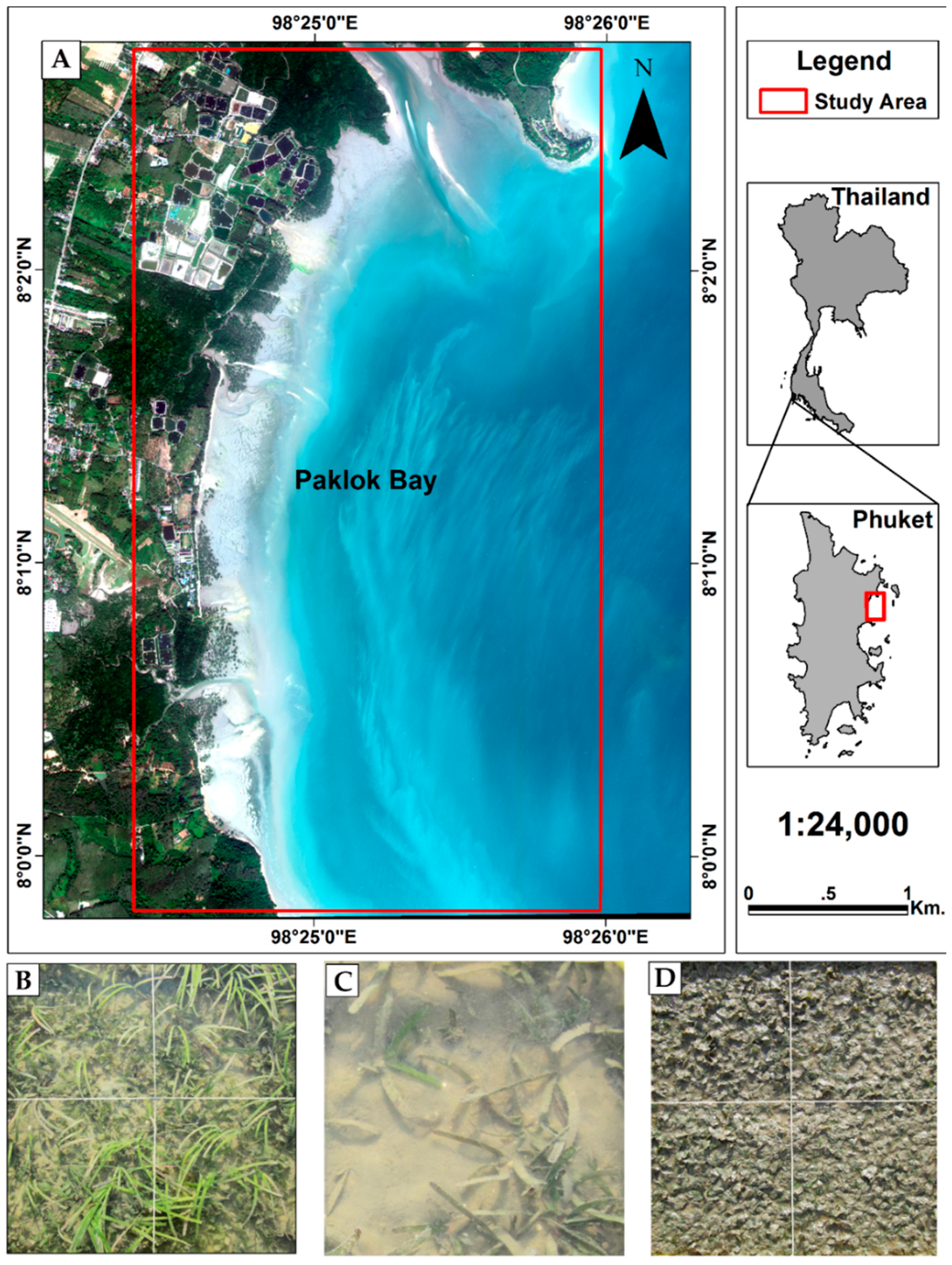
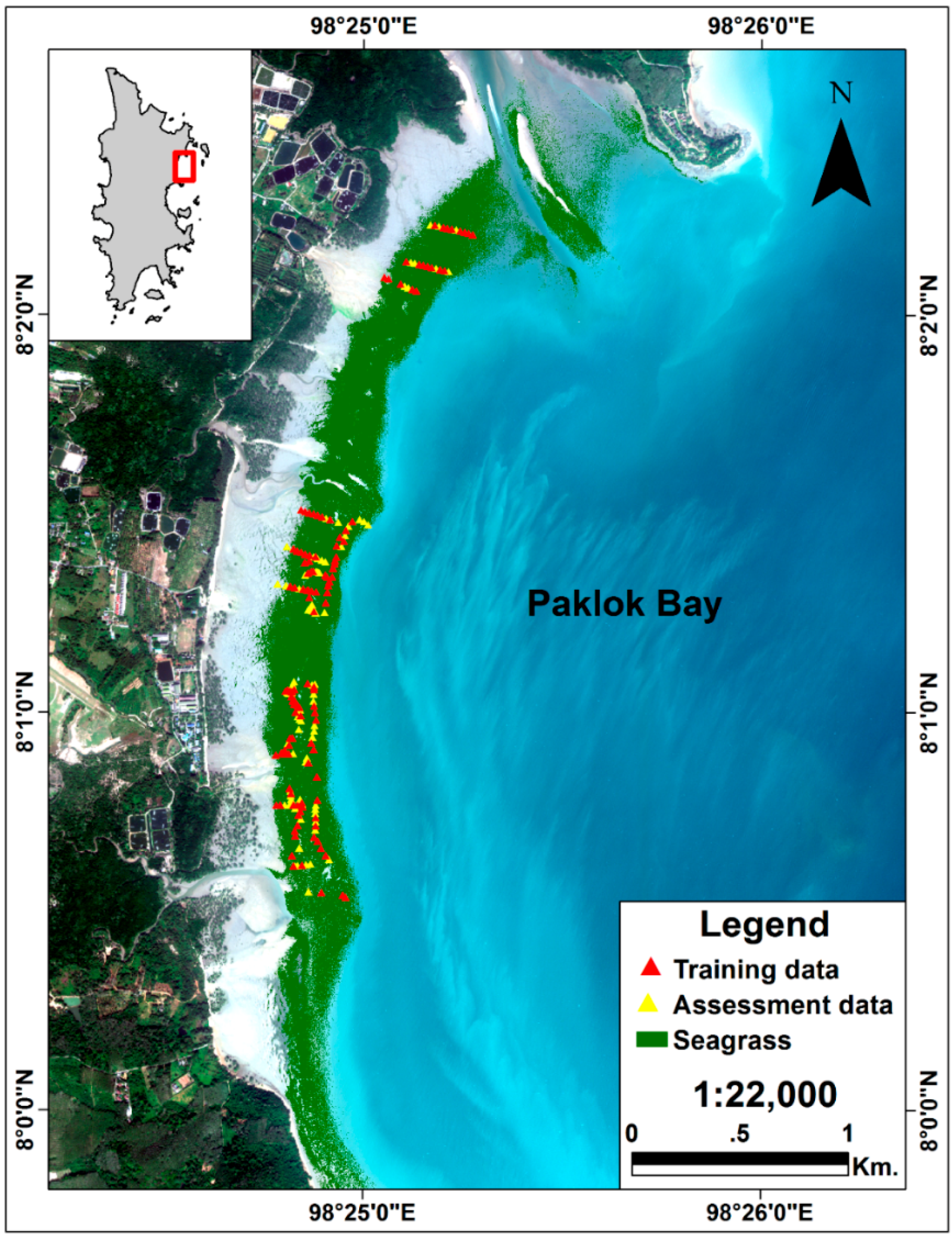
2.1. Study Site

The study site was at Paklok Bay, Talang District, Phuket province, in southern Thailand. It is located between 7°59’N and 8°3’N Latitude and 98°24’E and 98°27’E Longitude (Figure 1). The climate of the area is under monsoonal influence. There are two dominant seasons, a rainy season dominated by the Southwest Monsoon (typically from June to October) and a dry season when the Northeast Monsoon predominates (November to February). Strong winds and wave action during the southwest monsoon can be found along this coast [24]. Seagrass beds within Paklok Bay cover approximately 2.4 km² spread over an area 200 to 700 m from the shoreline. The seven documented seagrass species were Halodule uninervis, Halophila beccarii, Halophila ovalis, Cymodocea rotundata, Cymodocea serrulata, Thalassia hemprichii, and Enhalus acoroides [22]. The seagrass beds of the area are mostly found intertidally. Several shrimp (prawn) farms along the coast and rivers discharge turbid waters (Figure 1), which makes for difficulties in seagrass mapping.

2.2. Field Data Collection

The field data collection was carried out from 16 to 18 February 2014 under the protocols of the Survey Manual for Tropical Marine Resource [25]. This period was chosen for field data collection because of low tide conditions (i.e., approximately 1.0 m below mean sea level of Thailand) and also a 0.5 m water level difference with the satellite image acquisition time (i.e., approximately 1.5 m below mean sea level of Thailand). Line transect and some spot check methods were used for collecting spatially referenced benthic cover of the seagrass beds. Nine transect lines were chosen to cover the range of seagrass species and differences in the percentage cover levels throughout the seagrass area. The field data collected was used for the classification approaches and validation of the output seagrass maps. Digital photographs of 0.5 m × 0.5 m quadrats of the benthos (Photo-Quadrats) were captured at 20 m intervals for species and percentage cover.

The study area was characterized by small and patchy seagrass areas (especially, Halophila ovalis) with mixed species. If regular GPS was used the uncertainty would have been more than 10 meters horizontally and approximately 3 meters when using with Wide Area Augmentation System (WAAS) [23], but this technique was unavailable for the study area. Therefore, regular GPS was not appropriate for the study area. In the field we found that different cover types were very close together in small patches (i.e., each species of seagrass, sand, and mud). To make sure we correctly matched the spectral data from WV-2 and the geo-location of the field data, the coordinate of each of the sampling points was logged by a Topcon Hiper SR receiver using RTK positioning techniques (uncertainty less than one pixel of WV-2). The mapping control point was a station of the Thailand Department of Lands, located approximately 2 km away from the study area and used as the base station for positioning correction of RTK positioning technique. Three hundred and seventy data points were collected in total.

Above-ground seagrass biomass was measured in 0.5 m × 0.5 m quadrats of sample sites located at 40-m intervals along the transect line. The samples were returned to the laboratory where they were sorted out into stems and leaves and dried at 70 degrees Celsius for five days, and then weighed to produce an area weighted biomass estimate (g/m²) using standard methods [25].

Seagrass percentage cover and seagrass species were calculated through an assessment of each digital photograph using Coral Point Count with Excel Extensions 4.0 (CPCe) [26]. This was done by placing 100 points on each photo in the regular grid. For each point in the photo, the seagrass or substrate type (i.e., seagrass species, mud, sand, algae) was determined and entered in the CPCe program for calculation of the percentage cover and the assigned dominant species composition of seagrass. The species label could be only one specified dominant species (which had the highest percentage cover) or a mixed species label, if multiple species were abundant within the same sample point. In our survey, we found six of the seven seagrasses reported for the area, namely Halodule uninervis, Halophila ovalis, Cymodocea rotundata, Cymodocea serrulata, Thalassia hemprichii, and Enhalus acoroides, with three dominant species in terms of abundance (Enhalus acoroides, Halophila ovalis, and Thalassia hemprichii). Horizontally projected foliage cover of the seagrasses was calculated as a percentage of 100 points per photo-quadrat containing seagrass.

2.3. Remote-Sensing Data and Its Processing

A WV-2 (2 m spatial resolution) image with eight multispectral bands (

Table 1. Detailed information for Worldview-2 image data including the tidal level of the study area at acquisition time.

Worldview-2	Details
Date Acquired	27 December 2013
Time Acquired (Local)	10:24
Source	Digital Globe
Tidal level	−1.5 m
Spatial Resolution	2 m
Band ranges	Coastal: 400–450 nm
	Blue: 450–510 nm
	Green: 510–580 nm
	Yellow: 585–625 nm
	Red: 630–690 nm
	Red Edge: 705–745 nm
	NIR-1: 770–895 nm
	NIR-2: 860–1040 nm

) and an image acquisition date of 27 December 2013 was used in the study (Figure 1). The tide height at image acquisition was 1.5 m below mean sea level. The image was then re-projected into a UTM zone 47N and was geometrically corrected by using 16 ground control points (GCPs) gathered throughout the image, utilizing features that were easily identifiable landscape features. The aerial orthophoto (i.e., spatial resolution is 1 m) acquired in 2002 of the Phuket area, obtained from the Land Development Department, Ministry of Agriculture and Cooperatives, Thailand was used as the reference map for rectifying the WV-2 image. Under the geometric correction process, the nearest neighbor resampling technique was used for the geometric transformations to minimize the statistical properties changes of the datasets [27].

The Root Mean Square Error (RMSE) of the georectified image was below the size of one pixel of WV-2 (i.e., 0.33 pixel). Radiometric correction to normalize satellite images for factors such as sensor degradation, Earth-Sun distance variation, incidence angle, view angle, and time of data gathering were applied to the image data. The process involved converting Digital Number (DN) into radiance using calibration coefficients (i.e., gain and offset of each band) that accompanied with the image metadata. The image was then atmospherically corrected and transformed to reflectance using the MOD-TRAN-based FLAASH (Fast Line-of-sight Atmospheric Analysis of Spectral Hypercubes) algorithm. This study therefore did not need water column correction because most of the seagrass in the area was not submerged due to the very low tide at the time of the satellite image acquisition. Very little of the seagrass in Paklok Bay would not be accounted for in this survey because nearly all the seagrass (>90%) present grows intertidally [21]. Table 1 shows the summarized image details for the Worldview-2 images. The land areas above the high tide limit and water area at 2000 meters from the shore were masked in the final corrected image.

2.4. Spatial Distribution of Seagrass Areas

To define the extent of the seagrass beds, a spatial distribution map was produced using the Maximum Likelihood Classification (MLC) approach using commercially available software (ENVI version 5.0). A maximum likelihood classification algorithm is one of the well-known parametric classifiers used for supervised classification [28]. MLC relies on the second-order statistics of a Gaussian probability density function model for each class [29]. The advantage of the MLC as a parametric classifier is that it takes into account the variance-covariance within the class distributions and for normally distributed data, the MLC performs better than the other known parametric classifies [28]. Three discrete classes were classified (i.e., seagrass, sand, and deep water) by using reflectance values from WV-2 as input for the MLC algorithm. The deep water area refers to the area below the lowest low water sea level of the study area (≈2.5 m below extreme low tide). The 370 collected field data points were randomly divided into two groups of data points (60% and 40%, n = 220 & 150) for the purpose of image-supervised classification and validation. The map and reference data (i.e., validation data) were compiled into an error matrix and used to calculate overall, user, and producer accuracies [30]. The seagrass boundary map developed in this section was used to determine the area of seagrass percentage cover and the species maps.

2.5. Percentage Cover and Seagrass Species Mapping

The seagrass species and percentage cover maps were created using the MLC method. The reflectance values from WV-2 were used as input for the MLC approach. The seagrass cover refers to the horizontally projected foliage cover of the seagrass, in other words the area of substrate covered by seagrass when viewed directly from above [18]. Four discrete classes were classified: 0%–25%, 26%–50%, 51%–75%, and 76%–100%. A total of 261 data points were available for the four ranges of seagrass cover; the data points were randomly separated into two groups (60% & 40%) for training the supervised classification and accuracy assessment (i.e., 169 and 99 data points for classification and accuracy assessment, respectively).

The mapping process used was similar to the supervised classification applied to create seagrass cover maps, with a selection of the sample sites being used as training sites for the following dominant species classes: Enhalus acoroides, Halophila ovalis, and Thalassia hemprichii, as well as some commonly occurring mixtures of these species that were recognized from the photo-analysis results. The photo-quadrat photographs from the field survey were used to select areas appropriate as training sites for each seagrass species and substrate type. The sites dominated by individual species of seagrass were used to train the supervised classification. The total of 132 data points were available for classification (i.e., 80 and 52 data points for training and accuracy assessment, respectively). The seagrass boundary map developed in the previous section was used to determine the area of seagrass cover and the species maps (the deep water and sand classes were masked out).

2.6. Above-Ground Biomass Mapping

The Stepwise Multiple Linear Regression (SMLR) and Simple Linear Regression (SLR) analyses were applied to the above-ground seagrass biomass estimates, herein referred to as “biomass”. The reflectance values from the corrected WV-2 image were extracted for each of the biomass sample sites using all the available wavebands for the image. The 46 sample biomass values were entered as the dependent variable and the reflectance values as the independent variable for SMLR analysis. In addition, the seagrass percentage cover of each above-ground biomass sample points from the field data (i.e., 46 data points, after the high mixed species sample points were excluded) were applied as independent variables of SLR to the biomass estimates. Both methods (i.e., SMLR and SLR analysis) were applied to all species and for each species model. Finally, the resultant regression function was then applied to each pixel in the image for producing a map of above-ground seagrass biomass.

2.7. Accuracy Assessments

Accuracy assessments were conducted for the percentage cover of seagrass, species, and biomass maps based on validation data from the field photo-quadrat analyses. The error assessment procedure of percentage cover and species composition of seagrass followed standard satellite image processing protocols. The confusion matrices and summary tables containing the overall and individual class accuracies (i.e., producer’s and user’s accuracies) and kappa coefficients were generated using ENVI version 5.0. The correlation coefficient values (R), scatter plots, and Root Mean Square Error (RMSE) were analyzed to evaluate the accuracy of the biomass estimation.

3. Results

3.1. Spatial Distribution of Seagrass Area

The spatial distribution map of seagrass, sand, and deep water was produced using the MLC method of WV-2 spectral bands (Table 1). The accuracies of classification using different band combinations are shown in

Table 2. Maximum Likelihood Classification accuracies for mapping spatial distribution of seagrass using different spectral combinations. OA is the Overall Accuracy.

Bands Combination	Classification Accuracy
	OA (%)	Kappa
coastal, green, red edge, NIR-2	88.00	0.79
coastal, green, yellow, red edge, NIR-2	88.67	0.80
coastal, green, red, red edge, NIR-1, NIR-2	90.67	0.84

. The coastal blue, green, yellow, red-edge, NIR-1, and NIR-2 band combinations provided the best accuracies. The overall accuracy and kappa coefficient of the classification were 90.67% and 0.84%, respectively. The producer’s and user’s accuracy of each class and complete confusion matrix are shown in

Table 3. The confusion matrix and summary error statistics for seagrass distribution mapped from the Worldview-2 image validated against the field survey data. PA is Producer’s accuracy; UA is User’s accuracy. The gray area shows the confusion between seagrass and sand.

Classes	Seagrass	Sand	Deep Water	Total	UA (%)
Seagrass	78	11	0	89	87.64
Sand	3	38	0	41	92.68
Deep Water	0	0	20	20	100.00
Total	81	49	20	150
PA (%)	96.30	77.50	100.00

. The results in Table 3 indicate that the correct classification of seagrass by producer’s and user’s accuracy of seagrass was 87.64% and 96.30%, respectively. The classification results of the best spectral combination selected are illustrated in Figure 2. The seagrass bed is spread along the coast as a band approximately 200 to 700 m from the shoreline. The total seagrass area was approximately 1.50 square kilometers.

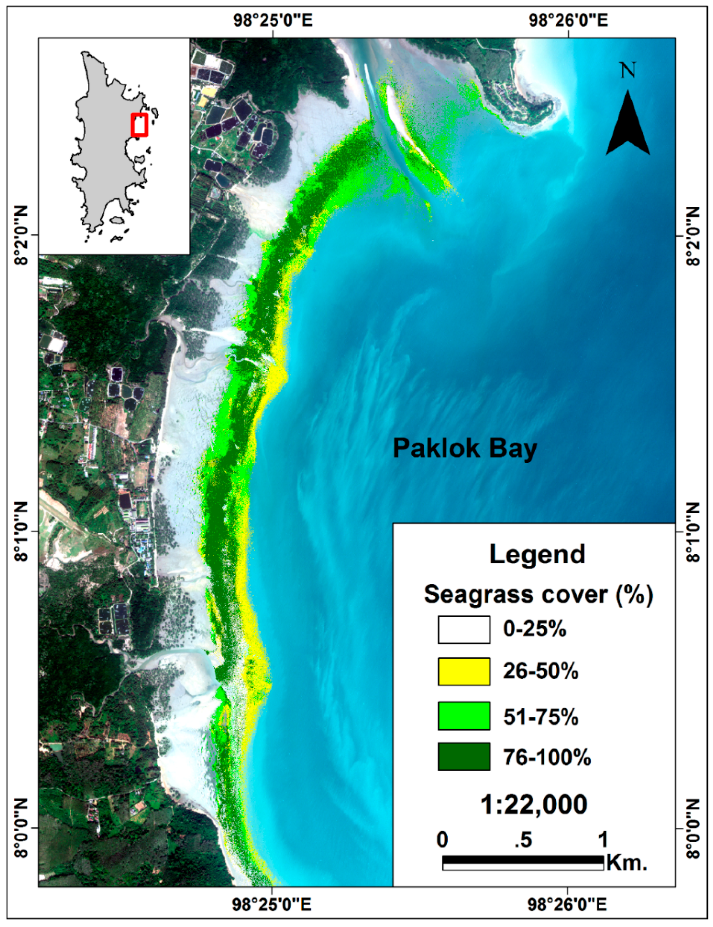
3.2. Percentage Cover Mapping

The MLC supervised classification was applied to create the spatial distribution of seagrass area maps. Four discrete classes were produced: 0%–25%, 26%–50%, 51%–75%, and 76%–100%. The 261 sample points were used for training the supervised classification and the rest of the sample points (i.e., 99 sample points) were used for an accuracy assessment. The classification accuracies from using different spectral combinations are shown in

Table 4. Maximum Likelihood Classification accuracies for mapping percentage seagrass cover using different spectral combinations. OA is the Overall Accuracy.

Band Combination	Classification Accuracy
	OA (%)	Kappa
coastal blue, blue, green, red, red-edge	68.69	0.57
coastal blue, green, red, red-edge, NIR-1	73.74	0.64
coastal blue, blue, green, red, red-edge, NIR-1	72.73	0.63

. The coastal, green, red, red-edge, and NIR-1 band combinations provided the best accuracy results (see wavebands in Table 1). The overall accuracy and kappa coefficient of the classification were 73.74% and 0.64%, respectively.

Table 5. The confusion matrix and summary error statistics for seagrass cover mapped from the Worldview-2 image validated against the reference field data of seagrass percentage cover estimated from photo transects. PA is Producer’s accuracy; UA is User’s.

Classes	0%–25%	26%–50%	51%–75%	76%–100%	Total	UA (%)
0%–25%	30	2	0	0	32	93.75
26%–50%	0	14	7	2	23	60.87
51%–75%	0	1	4	1	6	66.67
76%–100%	0	3	10	25	38	65.79
Total	30	20	21	28	99
PA (%)	100.00	70.00	19.05	89.29

lists the overall accuracy and producer’s and user’s accuracies produced using the test samples. Table 5 also shows the confusion factor between the 51%–75%, 26%–50%, and 76%–100% classes. Detailed seagrass cover classification maps (Figure 3) were created with the defined training and test samples. Figure 3 shows that approximately 70% of the seagrass area had a percentage cover lower than 76% (31% total area for 51%–75% covers, 32% total area for 26%–50% covers, and 7% total areas for 0%–25% covers). The area of dense seagrass cover (i.e., higher than 75% cover) was a long thin band spread along the shoreline in the central area of the seagrass area of the bay (dark green areas in Figure 3). The low cover patches (26%–50%) were mostly located in submerged areas and made a minor contribution to the total biomass.

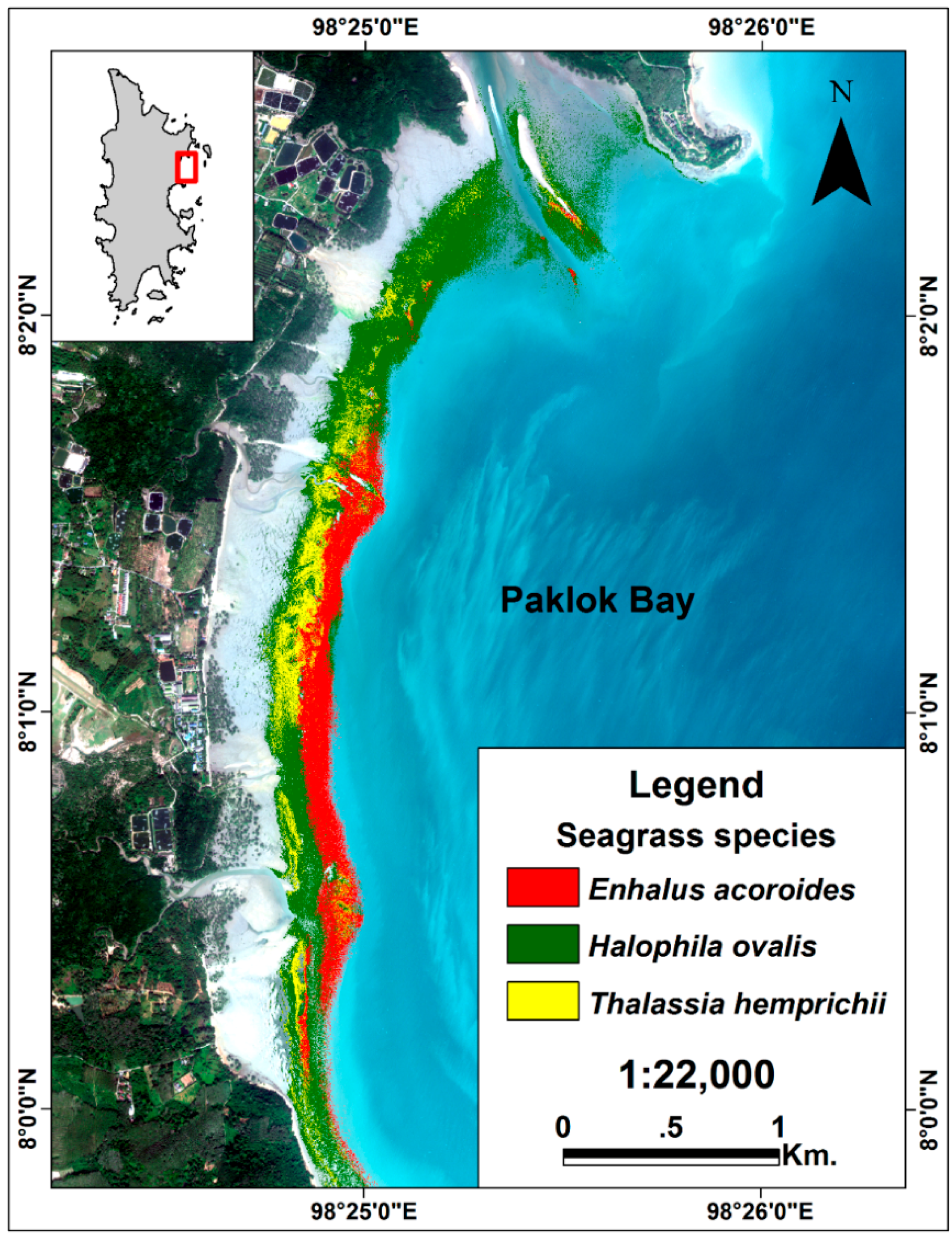
3.3. Seagrass Species Mapping

Three discrete classes of dominant species (i.e., Enhalus acoroides, Halophila ovalis, and Thalassia hemprichii) were classified using the MLC approach. The 80 sample points were used for training the supervised classification and the 52 sample points for accuracy assessment. The accuracy of classification using different combinations of spectral bands is presented in

Table 6. Maximum Likelihood Classification accuracies for seagrass species mapping using different spectral combinations. OA is the Overall Accuracy.

Bands Combination	Classification Accuracy
	OA (%)	Kappa
coastal blue, blue, green, red-edge, NIR-2	71.15	0.56
coastal blue, green, yellow, red-edge, NIR-2	75.00	0.61
coastal, green, red, red-edge, NIR-1, NIR-2	73.10	0.59

. The coastal blue, green, yellow, red-edge, and NIR-2 spectral band combinations yielded the best accuracy of classification. The overall accuracy and kappa coefficient of the classification were 75.00% and 0.61%, respectively.

Table 7. The confusion matrix and summary error statistics for seagrass species mapped from the Worldview-2 sensor validated against the field reference data of seagrass species estimated from photo transects. PA is Producer’s accuracy; UA is User’s accuracy. The gray area on the table shows the confusion between Enhalus acoroides and Halophila ovalis.

Classes	Enhalus acoroides	Halophila ovalis	Thalassia hemprichii	Total	UA (%)
Enhalus acoroides	19	5	6	30	63.33
Halophila ovalis	0	11	0	11	100.00
Thalassia hemprichii	1	1	9	11	81.82
Total	20	17	15	52
PA (%)	95.00	64.71	60.00

lists the overall accuracy and producer’s and user’s accuracies produced using the test samples. Table 7 also shows the confusion factor between species classes. The resulting seagrass species distribution map is shown in Figure 4. The map shows that the three dominant species are spread over the shoreline except around the north, where Enhalus acoroides was not found. Approximately 63%, 23%, and 14% of areas are covered by Halophila ovalis, Enhalus acoroides, and Thalassia hemprichii, respectively.

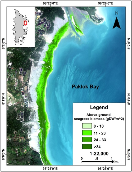
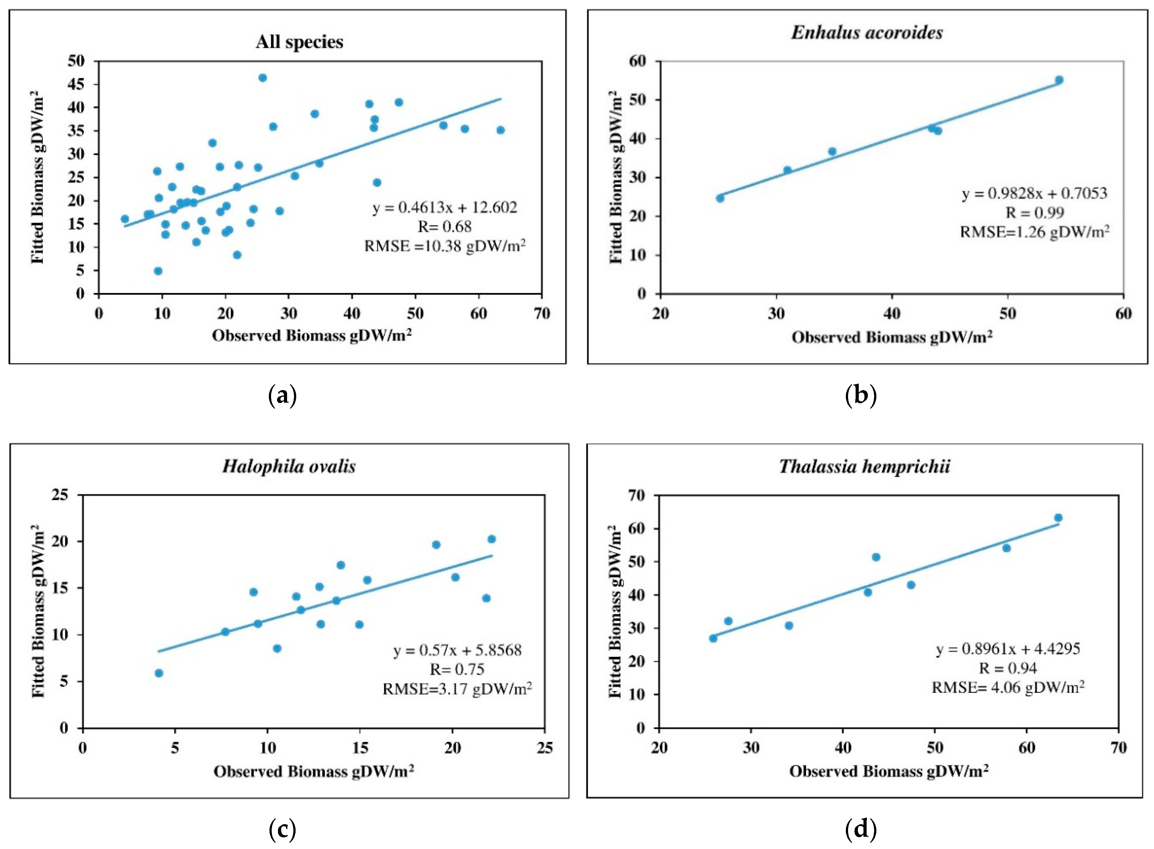
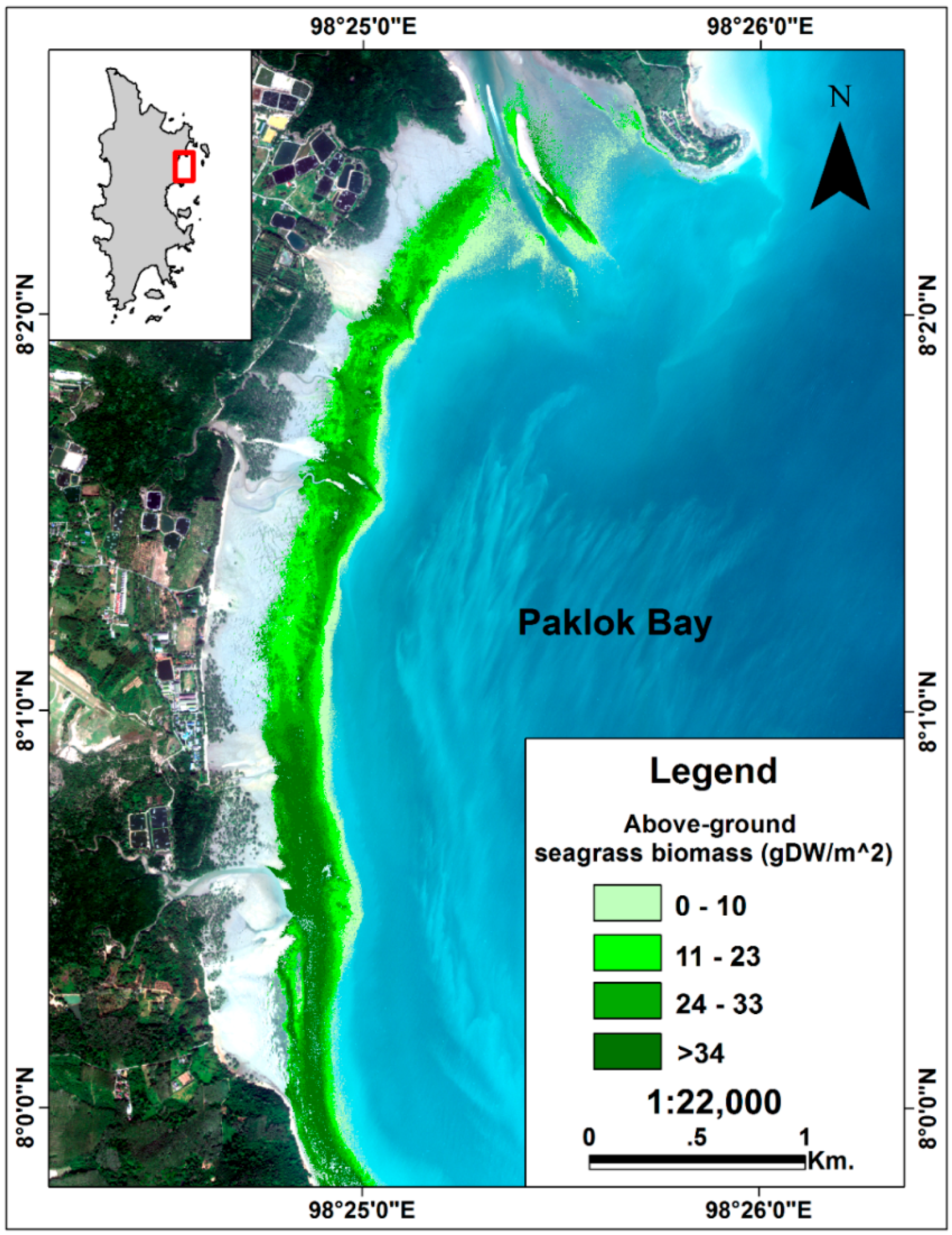
3.4. Above-Ground Biomass Mapping

3.4.1. SMLR Models with Spectral Bands as Independent Variables

The eight corrected spectral bands from WV-2 image and field biomass sampling points were used as the independent and dependent variables for SMLR analysis, respectively. For the whole species model, the analysis revealed the three most unique bands with the most information content to be green, yellow, and NIR-1; these bands were therefore used to estimate the above-ground biomass. An RMSE value of ±10.38 g/m² or ±10.38 tones/km² (R = 0.68) was calculated using the multiple linear regression model (see Figure 5a and

Table 8. The performance of models (R and Root Mean Square Error) for the above-ground biomass estimates of all species and Enhalus acoroides, Halophila ovalis, and Thalassia hemprichii species, where above-ground biomass was estimated by spectral bands and percentage cover.

Species	Estimated by Spectral Bands			Estimated by Percentage Cover
	Bands	R	RMSE (g·DW/m2)	R	RMSE (g·DW/m2)
All species	green, yellow, and NIR-1	0.68	10.38	0.13	14.01
Enhalus acoroides	coastal blue, blue, and yellow	0.99	1.26	0.94	3.09
Halophila ovalis	coastal blue, blue, yellow, and red-edge	0.75	3.17	0.80	2.90
Thalassia hemprichii	blue, green, yellow, and red-edge	0.94	4.06	0.67	9.34

).

The performance (R and RMSE) of estimation of above-ground biomass in each species model (i.e., Enhalus acoroides, Halophila ovalis, and Thalassia hemprichii) are shown in Table 8. The scatter plots of observed and estimated seagrass above ground biomass of all species, Enhalus acoroides, Halophila ovalis, and Thalassia hemprichii species are illustrated in Figure 5. The results in Table 8 and Figure 5 indicated that the performance of the SMLR models can be improved when analysis of each species is performed separately (RMSE are ±1.26, ±3.17, and ±4.06 g·DW/m² for Enhalus acoroides, Halophila ovalis, and Thalassia hemprichii, respectively). These errors for the separate species are very small when compared to the RMSE of ±10.38 g·DW/m² calculated from the pooled data.

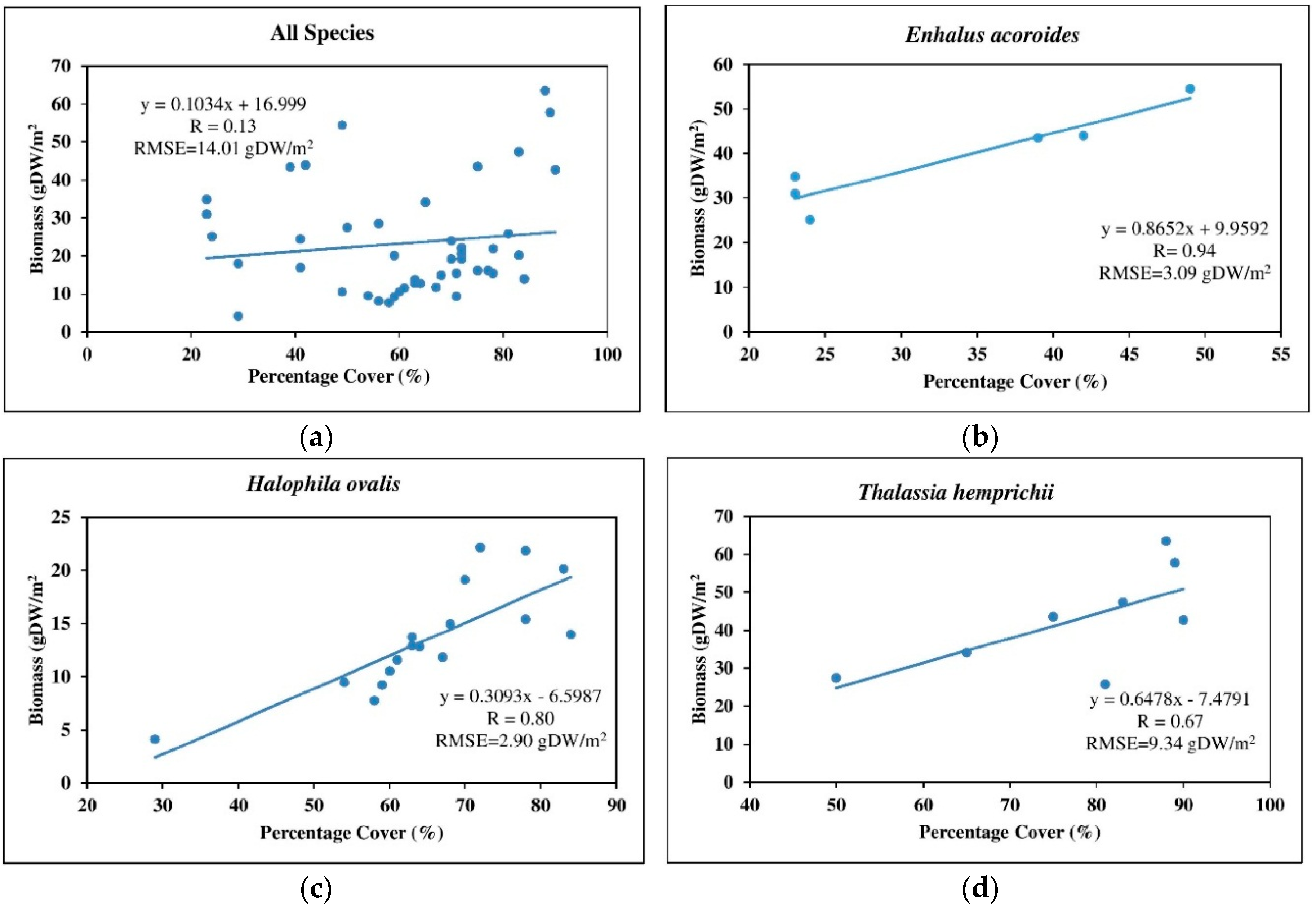
3.4.2. Simple Linear Regression with Percentage Cover as the Independent Variable

The percentage cover of each above ground biomass sample point was used as the independent variable for SLR analysis. The performance of each models (i.e., all species, Enhalus acoroides, Halophila ovalis, and Thalassia hemprichii species) are shown in Table 8. The scatter plots of seagrass percentage cover and seagrass above ground biomass of all species, Enhalus acoroides, Halophila ovalis, and Thalassia hemprichii species are illustrated in Figure 6. The results in Table 8 and Figure 6 indicated moderate to good relationships (R = 0.6–0.94) between seagrass percentage cover and above-ground biomass when each species was analyzed separately. In contrast, the results showed a poor relationship (R = 0.13) between seagrass percentage cover and above-ground biomass for the all species model where the information from each species was pooled.

In addition, the results in Table 8 showed that the spectral bands that were selected by SMLR analysis provided better results for the above-ground biomass of seagrass estimation percentage cover than the SLR analysis. Figure 7 shows the map produced from the global above-ground biomass model (i.e., all three dominant species within one model). Finally, total above-ground biomass values of each pixel per total area were calculated. The results showed that the overall average total of above-ground biomass per square kilometer was 23.95 tons·DW/km² or 23.95 g·DW/m² (calculated from the average of all seagrass pixels per total area of seagrass) with an error (RMSE) of ±10.38 tons·DW/km² or 10.38 g·DW/m².

4. Discussion

4.1. Spatial Distribution of Seagrass Area

The selected bands combination (i.e., coastal blue, green, yellow, red-edge, NIR-1, and NIR-2) provided high overall accuracy and kappa coefficient values (90.67% and 0.84%, respectively). We found that the Paklok Bay seagrass bed extended over an area approximately 200 to 700 m from the shoreline. This was in agreement with the ground survey report of the seagrass status of Phuket [22]. The total seagrass area was 1.50 km². Despite the fact that testing accuracy was as high as 90.67%, the study area was characterized by small and patchy seagrass areas with mixed species and several shrimp (prawn) farms along the coast discharging turbid waters (Figure 1), so there were still noticeable difficulties in discriminating between the seagrass class and the sand class (i.e., the highlighted area in Table 3).

4.2. Percentage Cover Mapping

The coastal blue, green, red, red-edge, and NIR-1 wavebands data produced the 0%–25%, 26%–50%, 51%–75%, and 76%–100% seagrass percentage cover with the best accuracy. The overall accuracy and kappa coefficient of the classification were 73.74% and 0.64%, respectively. This study achieved a higher accuracy than previous studies in Moreton Bay, Australia [18], which reported that seagrass cover mapping using Landsat 5 TM, QuickBird-2, and Airborne hyper-spectral (CASI-2) with four discrete classes (1%–10%,10%–40%, 40%–70%, and 70%–100%) only yielded 35.89%, 30.86%, and 45.64% accuracy, respectively. Later, Lyons et al. [12] reported accuracies of 59.00% and 62.00% for mapping cover of Moreton Bay between 2004 and 2007, whereas the recent study of Roelfsema et al. [10] reported that seagrass cover mapping of Moreton Bay, between 2004 and 2013 using WorldView-2, IKONOS, and Quickbird-2, had an average overall accuracy of 52%. Although this present study gained higher accuracy than previous studies of seagrass beds, it is hard to compare the accuracy with those three studies due to the differences of the environment, tidal level, satellite sensors used, and diversity of substrate, etc. In particular, in our study we were surveying a seagrass community restricted mostly to the intertidal zone and fully exposed at low tide. Most of the seagrass beds of Moreton Bay are subtidal. The leaves and stems of Enhalus acoroides species in Paklok Bay, which is generally located in the submerged area, did not project horizontally very well because its leaves do not lie flat on the substrate at low tide (Figure 1). This makes Enhalus acoroides difficult to measure or estimate in both field survey and by remote sensing methods.

4.3. Seagrass Species Mapping

The coastal blue, green, yellow, red-edge, and NIR-2 spectral channel combinations yielded the best accuracy of seagrass species classification (i.e., Enhalus acoroides, Halophila ovalis, and Thalassia hemprichii). The overall accuracy and kappa coefficient of the classification were 75.00% and 0.61%, respectively. Previous studies reported seagrass species mapping results of eight classes, using Quickbird and CASI, as only having 22.69% and 28.11% accuracies, respectively [18]. Lyons et al. [12] reported accuracies of 62.00% and 80.00% for mapping seagrass species of Moreton Bay (Australia) between 2004 and 2007 using Quickbird imagery. A recent study of Roelfsema et al. [10] achieved an averaged 77% species mapping accuracy (ranging from 71% to 83%) over 142 km² of shallow, clear water seagrass habitat (the Eastern Banks, Moreton Bay, Australia) using an object-based image analysis approach using Quickbird, Worldview-2, and IKONOS data. Although the present study achieved good accuracy, it is hard to compare our level of accuracy with the Moreton Bay studies due to differences of environments (e.g., size of the seagrass beds, the patchy distribution of seagrasses found in Paklok Bay, turbidity factors, tidal levels, diversity of substrates, and satellite data used, etc.). Despite the fact that we found a testing accuracy of 75% in our study, the difficulties in discriminating between the Halophila ovalis, Thalassia hemprichii, and Enhalus acoroides classes are still noticeable (i.e., the highlighted area in Table 7), resulting in low producer’s accuracy of the Halophila ovalis class. Morphologically Halophila is a very small seagrass compared to Thalassia and Enhalus. This discrepancy also reflects the actual situation of the Halophila ovalis class in the field, where it is usually mixed with Thalassia hemprichii as an undercover layer, making it difficult to detect and discriminate (Figure 1B).

4.4. Above-Ground Biomass Mapping

The results showed that the spectral bands selected by SMLR analysis provided better estimates of the above-ground biomass of seagrass estimation than seagrass percentage cover with SLR analysis. Although the models of each species are better than for pooled datasets of all species using both methods (i.e., spectral bands with SMLR and seagrass percentage cover with SLR), there is a need to correctly classify the seagrass species of the area before application of the regression results to produce the biomass map. Biomass estimation by SLR analysis with seagrass percentage cover as independent variables is also needed to correctly estimate the seagrass percentage cover of the area. The spectral bands selected by SMLR analysis (i.e., green, yellow, and NIR-1) were used to estimate the above-ground biomass for all species. The multiple linear regression model provided the RMSE value of ±10.38 g/m² or ±10.38 tons·DW/km² (R = 0.68) (see Figure 5). The characteristics of the study area (i.e., patch size, turbidity, percentage cover of seagrass, etc.) may have caused a lower accuracy of the model. Figure 3 shows that approximately 70% of the seagrass area has a percentage cover lower than 76%, with most of the seagrass area being mixed with sand. This makes it difficult to estimate the above-ground biomass from reflectance values because much of the total reflectance is from the sand rather than the biomass. This study reported the total above-ground biomass per square kilometer as 23.95 ± 10.38 g·DW/m² or 23.95 ± 10.38 tons·DW/km². These values were higher than a study by Nakaoka et al. [31] that reported an average above-ground biomass of eight seagrass species at Haad Chao Mai National Park, Trang Province Thailand as 15.37 g·DW/m² over intertidal areas and 10.64 g·DW/m² for subtidal areas. A recent study of the seagrass bed in Trang Province, Southern Thailand [29] reported that the highest total biomass in the lower intertidal zone was 32.68 ± 6.33 g·DW/m². The lowest total biomass in the subtidal zone and in the lower intertidal zone was 16.60 ± 0.64 g·DW/m². Their upper and lower values thus straddle the overall mean value found in the present study. The lowest total and above-ground biomasses in the subtidal zone were 2.87 ± 0.88 g DW/m² and 1.33 ± 0.36 g·DW/m², respectively.

Seagrasses as well as mangroves are in global decline [9,32,33]. Whereas declines of mangroves have been recently documented in SE Asia, information on seagrass decline in SE Asia and tropical regions in general is not well documented [9,32]. Much of the decline of mangroves in SE Asia has been a consequence of the expansion of aquaculture and agriculture and oil palm plantations [33], all of which impact upon seagrasses through runoff, sedimentation and eutrophication [34]. Increasing turbidity and nutrient concentration in water are considered to be the primary cause of seagrass loss [8]. Based mainly on North American, European, Caribbean, and Australian data, but no SE Asian data at all, estimates of the current global decline in seagrasses are on the order of 7% per year [9]. This study has shown that it is possible to monitor intertidal seagrass distribution, percentage cover, species, and biomass using remote sensing methods. The information of the distribution, percentage cover, species, and biomass of the seagrass are crucial information for improved management and protection of seagrass area. Documented global declines in seagrasses, the lack of broad-scale information in SE Asia, and the replacement of mangroves with oil palm plantations and aquaculture facilities in habitats generally immediately adjacent to seagrasses (Figure 1) show that there is an urgent need to map existing intertidal seagrasses in the region and monitor any degradation [8,9,33,34]. Intertidal seagrass beds are the more common type of seagrass bed found in monsoon SE Asia. Subtidal beds, found in clear water areas such as Trang, Thailand [16], could be mapped and monitored using methods developed for Moreton Bay in subtropical Australia [5,10,12,18]. Moreover, through the link between remotely sensed images and sediment and/or irradiance models, early warning systems may be developed to show those regions where growth conditions are deteriorating before the seagrass beds themselves display changes in cover or density [8]. In any case, monitoring the condition and extent of existing seagrass beds in SE Asia is a matter of urgency due to the large gap in information that is currently available.

5. Conclusions

This study confirmed the utility of high spatial resolution remote sensing data for mapping the spatial distribution, percentage cover, species composition, and above-ground biomass of intertidal seagrass in the south of Thailand, which is characterized by small and patchy seagrass areas with mixed dominant species, and generally turbid waters. Although most of the seagrass area was exposed, approximately 30% o was coated with silt-clay from turbid local watercourse discharge (Figure 1), which creates difficulties for seagrass mapping. We found that the spatial distribution of seagrass can be correctly classified despite the remaining confusion between seagrass and sand due to the characteristics of the study area (i.e., patch size, turbidity, percentage cover of seagrass, etc.).

In terms of percentage cover, the remaining confusion was in the 26%–50%, 51%–75%, and 76%–100% classes, which caused an overall moderate level of accuracy. Similarly, high spatial resolution satellite data provided only moderate overall accuracy for seagrass species mapping due to confusion between the Halophila ovalis, Thalassia hemprichii, and Enhalus acoroides classes. The cause of this confusion was an overall low percentage cover of seagrasses in the study area. As a result, the above-ground biomass model showed a lower accuracy than found in several previous studies, where seagrass beds had much higher biomass. This study used a higher accuracy positioning technique, the Real-Time Kinematic (RTK) Global Navigation Satellite System (GNSS), that has an uncertainty of less than one pixel of the WV-2 (<2 m), to record the position of field data. This resolves the difficulties in some previous studies [17] in matching locations between satellite images and field data sets. The acquisition date and time used in this study occurred at very low tide conditions in the study area, and thus most of the seagrass area was not submerged and this study did not have to correct for water column properties of subtidal seagrasses. It should be noted that the remote sensing processes used vary depending on the environmental conditions of the study area (i.e., elevation, tidal level, etc.) The systematic approach presented in this study used a combination of high spatial resolution (2 m pixel) multispectral satellite imagery and detailed field data to create seagrass distribution, species, percentage cover, and biomass maps. For ecologists and managers, the seagrass information in these high spatial resolution maps can provide invaluable information about seagrass ecology and can be used for the management of protected areas and understanding of biodiversity, functioning, services, and future sustainability of seagrass, particularly in the case of sparse seagrass beds.

References

1. Larkum, A.; Orth, R.J.; Duarte, C. Seagrasses: Biology, Ecology and Conservation; Springer: Dordrecht, The Netherlands, 2006. [Google Scholar]
2. Hossain, M.S.; Bujang, J.S.; Zakaria, M.H.; Hashim, M. The application of remote sensing to seagrass ecosystems: An overview and future research prospects. Int. J. Remote Sens. 2015, 36, 61–114. [Google Scholar] [CrossRef]
3. Knudby, A.; Nordlund, L. Remote sensing of seagrasses in a patchy multi-species environment. Int. J. Remote Sens. 2011, 32, 2227–2244. [Google Scholar] [CrossRef]
4. Orth, R.J.; Heck, K.L.; van Montfrans, J. Faunal communities in seagrass beds: A review of the influence of plant structure and prey characteristics on predator-prey relationships. Estuaries 1984, 7, 339–350. [Google Scholar] [CrossRef]
5. Roelfsema, C.M.; Phinn, S.R.; Udy, N.; Maxwell, P. An integrated field and remote sensing approach for mapping seagrass cover, Moreton Bay, Australia. J. Spat. Sci. 2009, 54, 45–62. [Google Scholar] [CrossRef]
6. Van der Heide, T.; van Nes, E.H.; Geerling, G.W.; Smolders, A.J.; Bouma, T.J.; van Katwijk, M.M. Positive feedbacks in seagrass ecosystems: Implications for success in conservation and restoration. Ecosystems 2007, 10, 1311–1322. [Google Scholar] [CrossRef]
7. Green, E.P.; Short, F.T. World Atlas of Seagrasses; University of California Press: Berkeley, CA, USA, 2003. [Google Scholar]
8. Ferwerda, J.G.; de Leeuw, J.; Atzberger, C.; Vekerdy, Z. Satellite-based monitoring of tropical seagrass vegetation: Current techniques and future developments. Hydrobiologia 2007, 591, 59–71. [Google Scholar] [CrossRef]
9. Waycott, M.; Duarte, C.M.; Carruthers, T.J.; Orth, R.J.; Dennison, W.C.; Olyarnik, S.; Calladine, A.; Fourqurean, J.W.; Heck, K.L.; Hughes, A.R. Accelerating loss of seagrasses across the globe threatens coastal ecosystems. Proc. Natl. Acad. Sci. USA 2009, 106, 12377–12381. [Google Scholar] [CrossRef] [PubMed] [Green Version]
10. Roelfsema, C.M.; Lyons, M.; Kovacs, E.M.; Maxwell, P.; Saunders, M.I.; Samper-Villarreal, J.; Phinn, S.R. Multi-temporal mapping of seagrass cover, species and biomass: A semi-automated object based image analysis approach. Remote Sens. Environ. 2014, 150, 172–187. [Google Scholar] [CrossRef]
11. Armstrong, R.A. Remote sensing of submerged vegetation canopies for biomass estimation. Int. J. Remote Sens. 1993, 14, 621–627. [Google Scholar] [CrossRef]
12. Lyons, M.; Phinn, S.; Roelfsema, C. Integrating Quickbird multi-spectral satellite and field data: Mapping bathymetry, seagrass cover, seagrass species and change in Moreton Bay, Australia in 2004 and 2007. Remote Sens. 2011, 3, 42–64. [Google Scholar] [CrossRef]
13. Howari, F.M.; Jordan, B.R.; Bouhouche, N.; Wyllie-Echeverria, S. Field and remote-sensing assessment of mangrove forests and seagrass beds in the Northwestern part of the United Arab Emirates. J. Coast. Res. 2009, 25, 48–56. [Google Scholar] [CrossRef]
14. Ferguson, R.L.; Wood, L.L.; Graham, D.B. Monitoring spatial change in seagrass habitat with aerial photography. Photogramm. Eng. Remote Sens. 1993, 59, 1033–1038. [Google Scholar]
15. Barillé, L.; Robin, M.; Harin, N.; Bargain, A.; Launeau, P. Increase in seagrass distribution at Bourgneuf Bay (France) detected by spatial remote sensing. Aquat. Bot. 2010, 92, 185–194. [Google Scholar] [CrossRef]
16. Kaewsrikhaw, R.; Ritchie, R.J.; Prathep, A. Variations of tidal exposures and seasons on growth, morphology, anatomy and physiology of the seagrass Halophila ovalis (R.Br.) Hook. f. in a seagrass bed in Trang Province, Southern Thailand. Aquat. Bot. 2016, 130, 11–20. [Google Scholar] [CrossRef]
17. Gullström, M.; de la Torre Castro, M.; Bandeira, S.O.; Björk, M.; Dahlberg, M.; Kautsky, N.; Rönnbäck, P.; Öhman, M.C. Seagrass ecosystems in the western Indian Ocean. AMBIO J. Hum. Environ. 2002, 31, 588–596. [Google Scholar] [CrossRef]
18. Phinn, S.; Roelfsema, C.; Dekker, A.; Brando, V.; Anstee, J. Mapping seagrass species, cover and biomass in shallow waters: An assessment of satellite multi-spectral and airborne hyper-spectral imaging systems in Moreton Bay (Australia). Remote Sens. Environ. 2008, 112, 3413–3425. [Google Scholar] [CrossRef]
19. Wolter, P.T.; Johnston, C.A.; Niemi, G.J. Mapping submergent aquatic vegetation in the US Great Lakes using Quickbird satellite data. Int. J. Remote Sens. 2005, 26, 5255–5274. [Google Scholar] [CrossRef]
20. Adulyanukosol, K.; Poovachiranon, S. Dugong (Dugong dugon) and seagrass in Thailand: Present status and future challenges. In Proceedings of the 3rd International Symposium SEASTAR and Asian Biologging Science, Bangkok, Thailand, 13–14 December 2006; pp. 41–50.
21. Poovachiranon, S.; Chansang, H. Community structure and biomass of seagrass beds in the Andaman Sea. I. Mangrove-associated seagrass beds. Phuket Mar. Biol. Cent. Res. Bull. 1994, 59, 53–64. [Google Scholar]
22. Department of Marine and Coastal Resources. The Survey and Assessment of the Status and Potential of Marine and Coastal Resources: Coral and Seagrass 2014; Department of Marine and Coastal Resources: Bangkok, Thailand, 2014. [Google Scholar]
23. El-Rabbany, A. Introduction to GPS: The Global Positioning System; Artech House: Norwood, MA, USA, 2002. [Google Scholar]
24. Wongkamhaeng, K.; Paphavasit, N.; Bussarawit, S.; Nabhitabhata, J. Seagrass gammarid amphipods of Libong Island, Trang Province, Thailand. Nat. Hist. J. Chulalongkorn Univ. 2009, 9, 69–83. [Google Scholar]
25. English, S.A.; Baker, V.J.; Wilkinson, C.R. Survey Manual for Tropical Marine Resources; Australian Institute of Marine Science: Townsville, QLD, Austrilia, 1997. [Google Scholar]
26. Kohler, K.E.; Gill, S.M. Coral point count with excel extensions (CPCe): A visual basic program for the determination of coral and substrate coverage using random point count methodology. Comput. Geosci. 2006, 32, 1259–1269. [Google Scholar] [CrossRef]
27. Foody, G.M.; Boyd, D.S.; Cutler, M.E. Predictive relations of tropical forest biomass from Landsat TM data and their transferability between regions. Remote Sens. Environ. 2003, 85, 463–474. [Google Scholar] [CrossRef]
28. ERDAS. ERDAS Field Guide; Erdas Inc.: Atlanta, GA, USA, 1999. [Google Scholar]
29. Paola, J.D.; Schowengerdt, R.A. A detailed comparison of backpropagation neural network and maximum-likelihood classifiers for urban land use classification. IEEE Trans. Geosci. Remote Sens. 1995, 33, 981–996. [Google Scholar] [CrossRef]
30. Congalton, R.G.; Green, K. Assessing the Accuracy of Remotely Sensed Data: Principles and Practices; CRC Press: Boca Raton, FL, USA, 2008. [Google Scholar]
31. Nakaoka, M.; Supanwanid, C. Quantitative estimation of the distribution and biomass of seagrass at Haad Chao Mai National Park, Trang Province, Thailand. Kasetsart Univ. Fish. Res. Bull. 2000, 22, 10–22. [Google Scholar]
32. Short, F.T.; Koch, E.W.; Creed, J.C.; Magalhaes, K.M.; Fernandez, E.; Gaeckle, J.L. SeagrassNet monitoring across the Americas: Case studies of seagrass decline. Mar. Ecol. 2006, 27, 277–289. [Google Scholar] [CrossRef]
33. Richards, D.R.; Friess, D.A. Rates and drivers of mangrove deforestation in Southeast Asia, 2000–2012. Proc. Natl. Acad. Sci. USA 2016, 113, 344–349. [Google Scholar] [CrossRef] [PubMed]
34. Burkholder, J.M.; Tomasko, D.A.; Touchette, B.W. Seagrasses and eutrophication. J. Exp. Mar. Biol. Ecol. 2007, 350, 46–72. [Google Scholar] [CrossRef]
Figure 1. (A) The satellite image of Paklok Bay captured by WV-2 sensor on 27 December 2013. The top left of the area shows the several shrimp farms along the shore that were sources of turbid waters; (B) Mixed dense seagrass; (C) sparse seagrass (Thalassia hemiprichii) with turbid waters; and (D) seagrass (Halophila ovalis) coated with silt-clay caused from the rivers discharge turbid waters.
Remotesensing 08 00292 g001
Figure 2. The seagrass area map for Paklok Bay derived from Worldview-2 image.
Remotesensing 08 00292 g002
Figure 3. The percentage cover of seagrass map for Paklok Bay derived from Worldview-2 image and field reference data.
Remotesensing 08 00292 g003
Figure 4. The dominant seagrass species map for Paklok Bay derived from Worldview-2 image and field reference data.
Remotesensing 08 00292 g004
Figure 5. Plot of observed vs. estimated seagrass above-ground biomass (g·DW/m2) using the multiple linear regression model for (a) all species; (b) Enhalus acoroides; (c) Halophila ovalis; and (d) Thalassia hemprichii. The observed above-ground biomass values are based on the field data gathered from 16 to 18 February 2014 in Paklok Bay.
Remotesensing 08 00292 g005
Figure 6. Plot of percentage cover vs. observed seagrass above=ground biomass (g·DW/m2) using the simple linear regression model for (a) all species; (b) Enhalus acoroides; (c) Halophila ovalis; and (d) Thalassia hemprichii. The observed above-ground biomass values are based the field data gathered from 16 to 18 February 2014 in Paklok Bay.
Remotesensing 08 00292 g006
Figure 7. The above-ground seagrass biomass map for Paklok Bay derived from Worldview-2 image and field reference data.
Remotesensing 08 00292 g007