Article

Mapping Plant Functional Types in Floodplain Wetlands: An Analysis of C-Band Polarimetric SAR Data from RADARSAT-2

by
Natalia S. Morandeira
1,2,*,
Francisco Grings
2,3,
Claudia Facchinetti
4,5 and
Patricia Kandus
1
1
Laboratorio de Ecología, Teledetección y Ecoinformática, Instituto de Investigación e Ingeniería Ambiental, Universidad Nacional de San Martín, 25 de Mayo and Francia S/N, General San Martín 1650, Buenos Aires, Argentina
2
Consejo Nacional de Investigaciones Científicas y Técnicas, Godoy Cruz 2290, Ciudad Autónoma de Buenos Aires 1425, Argentina
3
Grupo de Teledetección Cuantitativa, Instituto de Astronomía y Física del Espacio, Universidad de Buenos Aires—Consejo Nacional de Investigaciones Científicas y Técnicas, Intendente Güiraldes 2160, Ciudad Autónoma de Buenos Aires 1428, Argentina
4
Agenzia Spaziale Italiana, Via del Politecnico snc, Rome 00133, Italy
5
Instituto Gulich, Comisión Nacional de Actividades Espaciales, Ruta C45 km 8 Falda del Cañete, Córdoba 5187, Argentina
*
Author to whom correspondence should be addressed.
Remote Sens. 2016, 8(3), 174; https://doi.org/10.3390/rs8030174
Submission received: 17 November 2015 / Revised: 4 February 2016 / Accepted: 14 February 2016 / Published: 25 February 2016
(This article belongs to the Special Issue What can Remote Sensing Do for the Conservation of Wetlands?)

Abstract

:
The inclusion of functional approaches on wetland characterizations and on biodiversity assessments improves our understanding of ecosystem functioning. In the Lower Paraná River floodplain, we assessed the ability of C-band polarimetric SAR data of contrasting incidence angles to discriminate wetland areas dominated by different plant functional types (PFTs). Unsupervised H/α and H/A/α Wishart classifications were implemented on two RADARSAT-2 images differing in their incidence angles (FQ24 and FQ08). Obtained classes were assigned to the information classes (open water, bare soil and PFTs) by a priori labeling criteria that involved the expected interaction mechanisms between SAR signal and PFTs as well as the relative values of H and α. The product obtained with the shallow incidence angle scene had a higher accuracy than the one obtained with the steep incidence angle product (61.5% vs. 46.2%). We show how a systematic analysis of the H/A/α space can be used to improve the knowledge about the radar polarimetric response of herbaceous vegetation. The map obtained provides novel ecologically relevant information about plant strategies dominating the floodplain. Since the obtained classes can be interpreted in terms of their functional features, the approach is a valuable tool for predicting vegetation response to floods, anthropic impacts and climate change.

Graphical Abstract

1. Introduction

The largest wetlands of South America are associated with the floodplains of the Amazonas, Orinoco and Paraná-Paraguay Rivers [1]. These ecosystems feature high biodiversity and are important for society due to flood regulation, habitat provision for fish and wildlife, natural forage provision for cattle, and carbon sequestering, among other factors [2,3]. Floodplain wetlands have been mapped and monitored with optic data in several opportunities (e.g., [4,5,6]). However, optical data often fail in the discrimination of vegetation types, especially if signal saturation occurs because of the dominance of herbaceous plants with high coverage and dense biomass [7,8].
In the last decades, Synthetic Aperture Radar (SAR) data have been noted as a promising tool to discriminate wetland vegetation types and to assess their dynamics, mainly due to the ability to detect water below the vegetation [8,9,10,11]. Nevertheless, most SAR applications in wetlands have been developed in forests [11,12], and few works are focused specifically on herbaceous wetlands (e.g., [13,14]). In the Paraná River floodplain, the downstream deltaic portion has been addressed with SAR data using conventional techniques [6,15,16,17].
Most of the Middle and Lower Paraná River floodplain is dominated by herbaceous plant communities [18,19]. To discriminate among different wetland herbaceous vegetation types, the available knowledge suggests that C-band data are preferred to L-band data, cross-polarizations to co-polarizations and shallow incidence angles to steep ones [7,11,12,20,21,22]. The experience on the extraction of polarimetric information and on polarimetric classifications is scarce in wetland ecosystems [23]. Most of the studies using polarimetric data are based on the use of multipolarization information (HH/HV/VV) (the first and second letters denote transmit and receive polarizations, respectively; with H denoting horizontal and V vertical polarizations) or on the analyses of polarimetric indexes [9,24,25,26,27,28,29,30]. The information in the complex coherence or covariance matrices is usually under-exploited [31] and only recent works in wetland ecosystems have used complex polarimetric matrices [32,33,34,35,36,37,38,39].
Wetland land-cover classes to be classified may differ according to the objective of the study. Here we propose mapping plant functional types (PFTs), which can be defined as “sets of species showing similar responses to the environment and similar effects on ecosystem functioning” [40]. Although remote sensing with SAR data has not been widely used to discriminate PFTs [41], PFT detection may be possible if their functions are associated with structural traits (leaf area, number of leaves, plant height, etc.). The spatial distribution of PFTs can be used as an indicator of the wetland state, especially if the maps obtained are coupled to an assessment of PFT responses to environmental changes and disturbances. In addition, the inclusion of the functional component in biodiversity assessments highly improves the understanding of ecosystem functioning [42,43,44]. In floodplain wetlands, plant strategies such as PFT have been proposed as a tool to predict direct and indirect effects of floods, such as nutrient limitation or excess, or the disturbances generated by erosion or deposition processes [45].
Our aim was to assess the use of C-band polarimetric SAR data of contrasting incidence angles to discriminate wetland areas dominated by different PFTs in the Lower Paraná River floodplain. The main hypothesis was that C-band signal interacted differentially with different PFTs summarizing not only structural but also functional features of the vegetation. In addition, we expected that the interaction between the SAR signal and the PFTs differed according to the incidence angle. Unsupervised H/α and H/A/α Wishart classifications were performed and the accuracy obtained with contrasting incidence angles was compared.

2. Materials and Methods
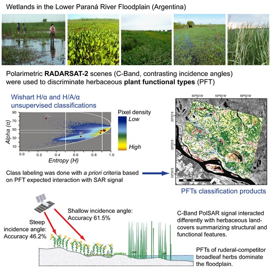
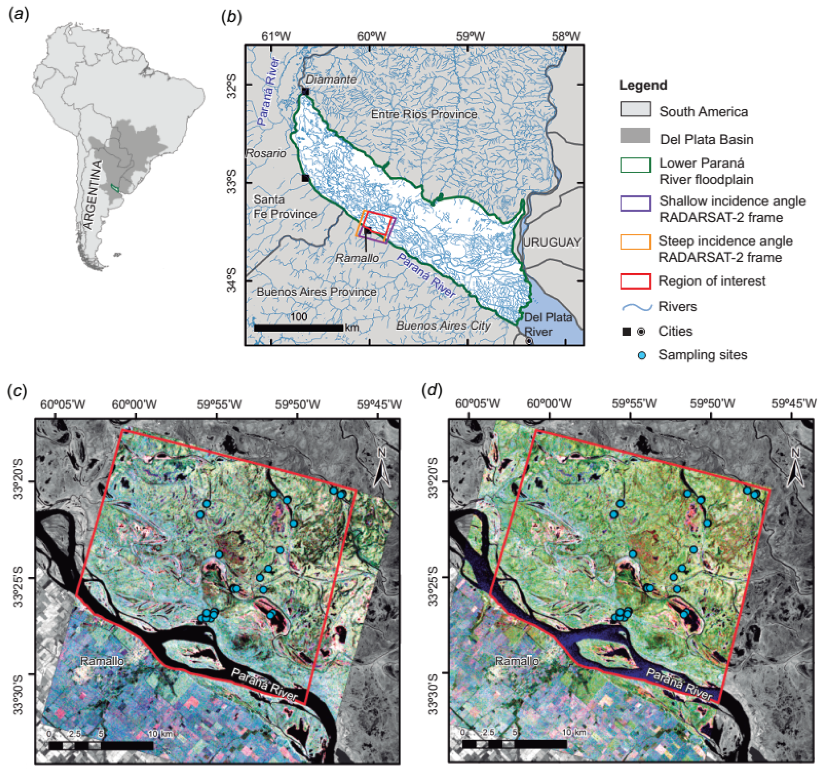
2.1. Study Area

The study was conducted in an area of the Lower Paraná River floodplain (Figure 1), which is subject to the flood pulse of the Paraná River. The climate is temperate humid, the mean annual temperature is 17.1 °C, January being the hottest month and July the coldest (24.0 °C and 10.3 °C, respectively). The mean annual precipitation is 1054 mm, March being the wettest month and August the driest (131.4 mm and 40.7 mm, respectively) (1965–2013; Instituto Nacional de Tecnología Agropecuaria (INTA) San Pedro Agrometeorological Station, 33°44′S–59°41′W). The area is relatively flat: the mean difference between high and low positions at a local scale is 65 cm (sensu records in 17 transects, measured with a laser level by Morandeira and Kandus). Herbaceous communities dominate marshes, whereas forest patches cover ca. 1.5% of the study area [46]. Marsh communities are distributed with a zonation pattern, with well-defined limits between vegetation zones and few species with high dominance at a local scale [18]. The main commercial activity is cattle ranching, which depends on the natural herbaceous vegetation of the area. Secondary commercial activities are fishing and apiculture.

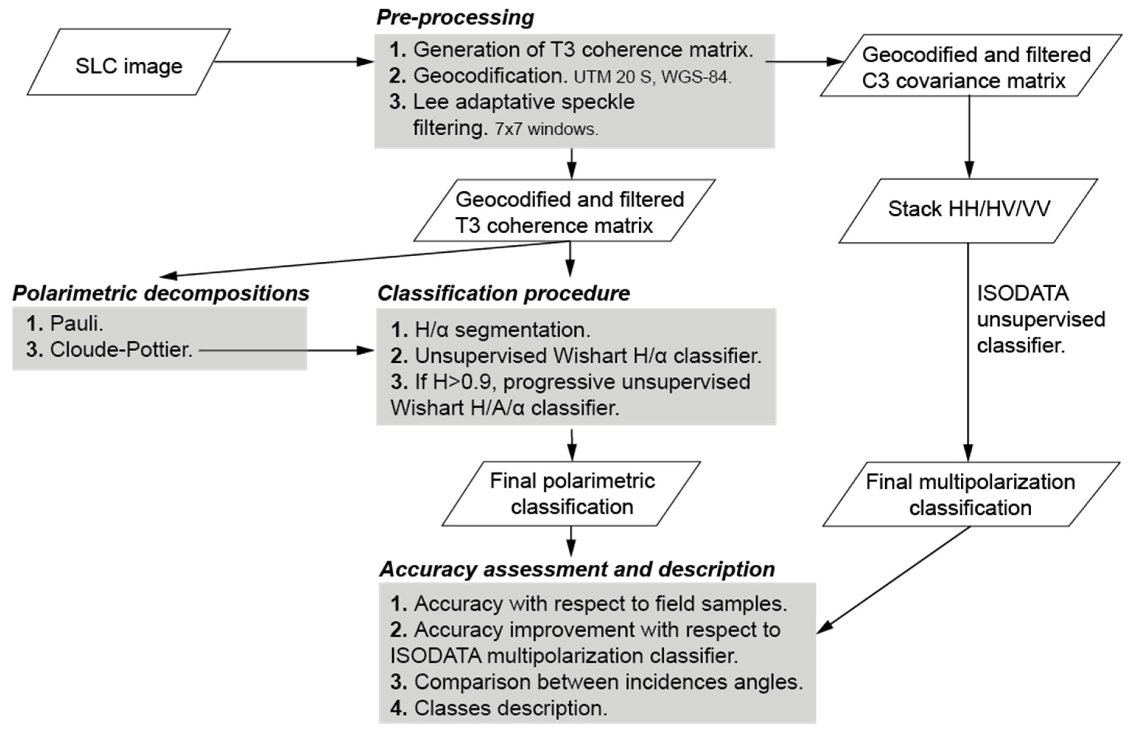
2.2. SAR Data Acquisition and Processing

Two polarimetric RADARSAT-2 scenes (C-band, frequency 5.405 GHz, wavelength 5.6 cm) were acquired on 30 January and 2 February, 2011 (Table 1). The overlapping area of the scenes acquired covers 462 km2 of freshwater wetlands, resulting in the region of interest for further analyses (Figure 1). Incidence angles were contrasting: the first scene had a relatively shallow incidence angle (Beam FQ24) and the second one a steep incidence angle (FQ8) (Table 1). Between acquisition dates, the accumulated precipitation was negligible (2 mm, data from Servicio Meterológico Nacional (SMN), Argentina) and hydrometric level in the Paraná River increased only 13 cm (data from Prefectura Naval Argentina), remaining far below the level for which water begins to enter the floodplain [47]. Wind speed and wind direction (which can affect water roughness and the orientation of plant leaves) were similar in the two dates: gentle breezes between 12 and 15 km/h with east or northeast direction (data from SMN). Thus, backscattering differences between scenes were assigned only to the differing incidence angle.
Figure 2 shows a flow diagram for the pre-processing and processing of the two RADARSAT-2 scenes. PolSARpro [48] was chosen for most of the steps, since it can handle coherence and covariance matrices, filters, decompositions, segmentations, classifications and statistical analyses. Each SLC scene was imported and digital numbers were converted to sigma-nought values. Next, the T3 coherence matrix and the C3 covariance matrix were geocodified with MapReady [49]. Since the study area is relatively flat, no terrain correction with a digital elevation model was applied. The images were filtered for speckle reduction using the adaptive Lee filter [50] with a 7 × 7 pixel window size. Geocoding before filtering diminished image artifacts. The intensities of the backscattering coefficients in HH, HV and VV were extracted and transformed to decibels (dB). Note that HV = VH if reciprocal targets are assumed [51].

2.3. Classification of Areas Dominated by Plant Functional Types

2.3.1. Information Classes: Sampling and Characterization

Vegetation sampling was conducted during the summers of 2010–2011 and 2011–2012 in 39 georeferenced sampling sites distributed along the region of interest (Figure 1c,d). Dominant plant species were classified into plant functional types (PFTs) by means of a trait-based approach. The PFT classification was derived from a broader study, in which 16 functional traits were screened in 44 species that dominated 72 sites (39 sites in the study area of this work and 33 sites in surrounding areas of the Paraná River floodplain) (Morandeira and Kandus, in prep.). For some species, more than one population was sampled. Next, these populations were hierarchically classified into PFTs. Thus, we consider that the identified PFTs were representative of the Lower Paraná River floodplain. PFTs were characterized and assigned to a life strategy (competitor, ruderal, or stress-tolerant) [52,53] by interpreting their mean trait values and trait ranges. Five PFTs covered homogeneous areas of at least 1000 m2 in the study area of this work, and are described in Table 2. The location of three sites with bare soil (cattle corrals or areas with high cattle transit) and of ten sites of open water (shallow lakes and rivers) was also recorded. This led to a total of 52 field observations, which were used for accuracy assessments in next steps. Site selection was limited by accessibility, but was independent of classification results (sampling was conducted before performing the classifications). Homogenous areas around these georeferenced sites were identified by visual interpretation of Pauli representations [51] derived from each scene. In order to assess whether the information classes (PFTs, bare soil and water) can be differenced by their backscattering coefficients in HH, HV and VV, permutation ANOVAs (999 permutations) followed by a posteriori Tukey’s tests [54] were carried out. Permutation ANOVAs were run with the open-source software R [55] and the package lmPerm [54].

2.3.2. H/A/α Segmentation

The Cloude–Pottier polarimetric decomposition expresses the 3 × 3 complex coherence matrix as a sum of eigenvalues (λi) and eigenvectors ( e i ¯ ) [56]. Three components can be obtained from the T3 matrix: entropy (H), angle α and anisotropy (A) [57]. The entropy ranges between 0 and 1: values near 0 indicate a single scattering mechanism, whereas values near 1 indicate a random combination of different scatterers [56]. The average α component ranges between 0° and 90° and depends on the dominant scattering mechanism: surface scattering for values near 0°, dipole scattering for values near 45° and double-bounce scattering for values near 90° [58]. Lastly, low A values are obtained for a main scattering mechanism (case H = 0 or H = 1) and two non-negligible secondary mechanisms, whereas high A values correspond to two main scattering mechanisms with the same probability of occurrence and a third mechanism of minor importance [59].
After extracting the three Cloude–Pottier components, the pixel density distribution of each scene was plotted in an H/α plane. An H/α segmentation was obtained by dividing the plane into nine zones (a combination of low/medium/high H and low/medium/high α) [56]. Thresholds between the zones are somewhat arbitrary. A curve delimits mathematically infeasible solutions (high H and low α), so that eight zones remain feasible. By introducing A, it is possible to obtain two H/α planes, one for A > 0.5 and the other for A < 0.5. Thus, an H/A/α segmentation leads to 16 zones with distinct scattering behavior.

2.3.3. Wishart Unsupervised Classifications on the Coherence Matrix

The Wishart H/α or H/A/α unsupervised classifiers are non-hierarchical statistical algorithms that require a Cloude–Pottier segmentation product [58]. In each scene, iteration optimization procedures were initialized from the centroids of the H/α or of the H/A/α segmentations (8 or 16 feasible classes, respectively). The classifications were computed on the T3 matrix by means of a complex algorithm based on the Maximum Likelihood classifier, with a convergence level of 99%, a maximum of 100 iterations and a 3 × 3 pixel window size. Thus, two Wishart unsupervised classifications were obtained for each scene, one derived from the H/α plane and the other from the H/A/α plane.
Classes derived from the unsupervised H/α classification were assigned to the information classes (water, bare soil or a PFT) according to their H and α values and following a priori predictions. We considered that H increased with randomness and geometric anisotropy of the scatterers, whereas α varied with the dominant interaction mechanism between the signal and the target (low α for surface scattering, medium α for volume scattering and high α for double-bounce scattering). The water information class was expected to have low values of both H and α, and to be identified due to the known location of the main rivers and shallow lakes. Surface incoherent scattering was expected in bare soil targets, with low α and intermediate H values. Regarding PFTs, those presenting double-bounce scattering (mainly due to vertical stems) were expected to show the highest α (PFT A). Previous works have addressed the contribution of double-bounce scattering in Schoenoplectus californicus [60], which is a species included in PFT A and with a similar structure to Cyperus giganteus. Besides, the overall biomass and the degree of randomness in the canopy (distribution of leaves and stems) were assumed to be related to H (see Table 2 for predictions of the scattering mechanisms of PFTs). PFTs with broadleaf leaves and stems were expected to have higher randomness in biomass distribution (particularly PFT C, but also PFT B), and biomass was expected to be related to volume scattering. In this sense, we assigned Wishart classes to PFTs assuming an increasing order of H: PFT D < PFT E < PFT B < PFT C, from short and low biomass grasslands (PFT D) to tall and high biomass broadleaf marshes (PFT C). Dihedral scatterers such as ships or buildings were associated to very high α and very low H (these targets occurred in the segmented scenes but were outside the overlapping study area). This labeling procedure was a working hypothesis: the expected H and α values for different information classes could be inferred from the structural features of the targets. Accuracy assessment with field data (see Section 2.3.4) was used to discuss whether this hypothesis was accurate for our purpose. A second class labeling procedure, not associated with hypotheses on the vegetation–signal interaction, was conducted by maximizing the Kappa index.
The discrimination of targets with high entropy might be improved by including the anisotropy component (as suggested by [51]). Thus, a progressive classification procedure was carried out for those classes derived from the H/α Wishart classification with very high entropy values (H > 0.90). The H/α Wishart classes were further divided taking into account the classes from the unsupervised H/A/α Wishart classification. Next, whether PFT discrimination was improved using H/A/α classes to re-allocate pixels to the information classes was analyzed.

2.3.4. Accuracy Assessment

The accuracy of the Wishart unsupervised classifications was assessed in the 52 georeferenced sampling sites included in the region of interest (39 sites of PFTs, three of bare soil, ten of open water) (see Section 2.3.1 for details on site sampling). Overall accuracy was computed as the number of pixels correctly classified out of the total number of pixels. To evaluate how much the resulting accuracy differed from a random assignment of class labels, the Kappa index was computed [61]. The accuracy observed was also expressed as the proportion of the accuracy that may be obtained with an easier and simpler classification (“naïve” classification, sensu [62]). In this study, the accuracy of a straightforward Isodata unsupervised clustering of SAR data expressed in the canonical polarization base was considered for comparison purposes [63]. The Isodata classification was carried out on the pixels of the multipolarization stack (HH, HV and VV) (seven classes, 100 iterations or a convergence level of 0.99). A median filter with a 3 × 3 window was applied on the product of the Isodata classification so that it could be compared to the Wishart product. Both Wishart and Isodata are non-hierarchical classifiers and compute the distances of the pixels to their respective clusters centroids in each of the iterations. Thus, the accuracy of the Wishart classification compared to the accuracy of this multipolarization stack might be understood as a measure of the improvement of the classification due to the use of the complex polarimetric information contained in the T3 matrix. This is particularly important, since polarimetric information extraction techniques are more complex and time-costly and therefore their use should be justified.

3. Results and Discussion

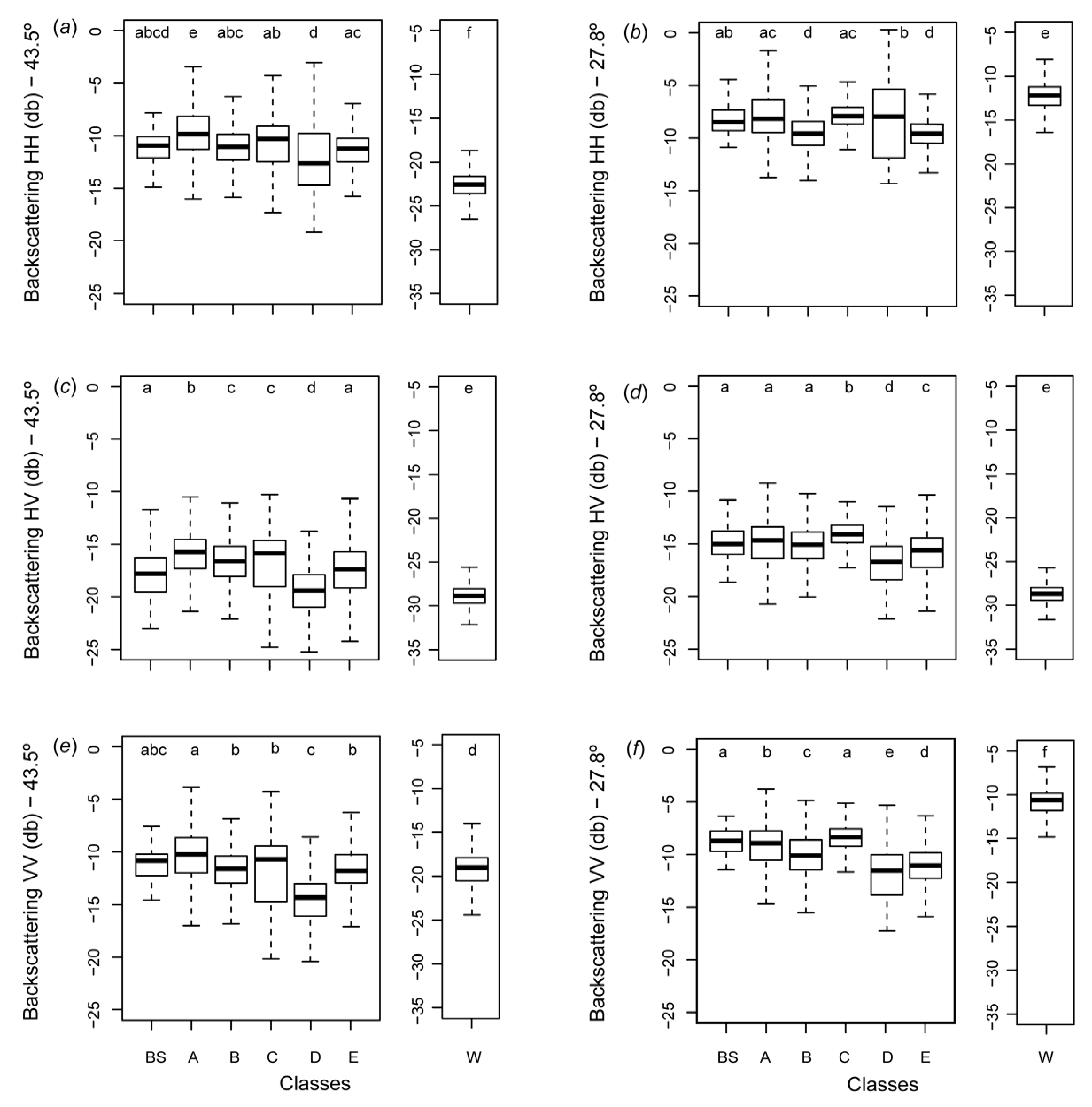
3.1. Description of the Scenes and Field Samples

In both RADARSAT-2 scenes, co-polarizations (HH and VV) showed similar backscattering coefficients for most of the field samples belonging to different classes (Figure 3), except for PFT E (tall grasslands, see Table 2) for which backscattering was higher and more variable in HH than in VV. The analysis of field samples representative of each class suggests that using only one polarization is quite inappropriate for classifying the region of interest, especially with regard to bare soil discrimination (Figure 3). However, HV (or VH) seems to be the preferred polarization for discriminating wetland classes with RADARSAT-2 scenes. Differences between information classes were higher in the cross-polarization band (HV) than in co-polarization bands (HH or VV). This issue has been pointed out in [11]: the depolarizing character of the vegetation differs according to vegetation structure, biomass distribution and flooding state.
Characterized mainly by mirror reflection, water had low backscattering coefficients. However, water scattering was higher in the steep angle scene than in the shallow one, as expected for a slightly rough surface. The highest backscattering was observed for PFT A samples (bulrush marshes), probably due to the contribution of double-bounce scattering that was reported and modeled in [60]. The lowest scattering among vegetation classes occurred for PFT D, grouping short plants with low cover and biomass, which probably allowed large signal penetration up to rough soil or water. Bare soil backscattering was always similar to the backscatter of at least one PFT, thus suggesting difficulty to discriminate bare soil in further classifications (especially if polarimetric information is not included). Although the backscattering of some classes showed differences between the scenes (Figure 3), these differences were not evident in the Pauli representations (Figure 1c,d) and high cross-polarization response (high |HV|) predominated in both scenes.

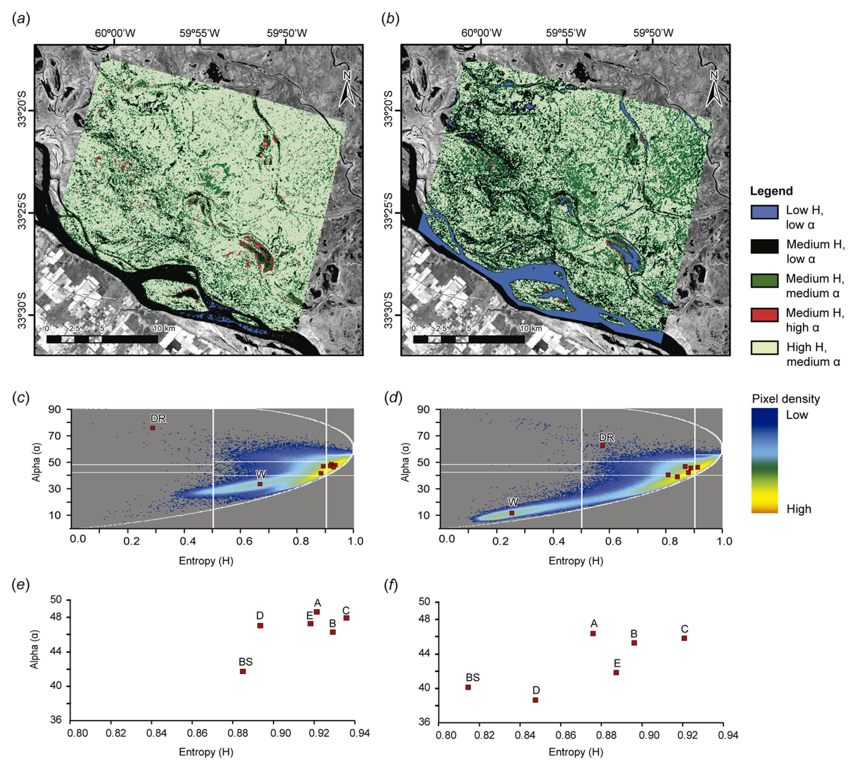
3.2. H/α Segmentations

The interaction between PFT targets and the polarimetric SAR signal was heavily influenced by the incidence angle (Figure 4), assuming no substantial changes in vegetation, hydrometric or wind conditions during the two days between scene acquisitions (see Section 2.2). In line with the predominance of volume scattering at C-Band from vigorous herbaceous vegetation, most of the pixels of both scenes had high H (H > 0.8) and intermediate α values (30° < α < 50°). Thus, segmenting the H/α plane in eight zones was not accurate for discriminating PFTs and bare soil: the non-water areas were grouped in the same class in both segmented images (Figure 4a,b). The density of pixels in zones with low α and low or intermediate H, thus presenting simple interaction mechanisms, was higher in the steep angle scene than in the shallow angle scene (Figure 4c vs. Figure 4d). In the segmented image from the steep angle scene (Figure 4b), those pixels were located in wetland areas with high H values in the shallow angle scene. These differential signal-target interactions according to the incidence angle may indicate the presence of flooded vegetation. Indeed, with a shallow incidence angle, volume scattering with one or more vegetation layers occurred, so that the signal was scattered before reaching water below vegetation. On the contrary, the steep signal was less attenuated by the vegetation and mainly interacted with water below it.
Few pixels with high α (indicating double-bounce scattering) occurred in both scenes. The ones with low H were located in the middle of the Paraná River or outside the region of interest in urban areas, pointing out dihedral reflectors (e.g., ships, buildings, metal roofs). Besides, the pixels with high α and intermediate or high H were probably related to double-bounce from vegetation targets. Their locations were coincident in both segmented images, but the covered area was slightly higher in the shallow incidence angle scene than in the steep one.
These analyses of the H/α space improved the previous knowledge about the response of herbaceous wetland vegetation to SAR signal. Most of the previous studies have described high H areas as forests and high α areas as cities (e.g., [23,64,65]). However, high biomass vegetation assessed in this study featured very high H. According to the a priori labeling criteria, the location of the PFT A pixels in the H/α plane was similar to the location of pixels with floodable trees and shrubs in the Amazonas floodplain [32]. High α values in pixels dominated by the equisetoid herbs of PFT A (e.g., Schoenoplectus californicus in bulrush marshes) presented high α values such as predicted due to its high double-bounce scattering in presence of a water film [60].

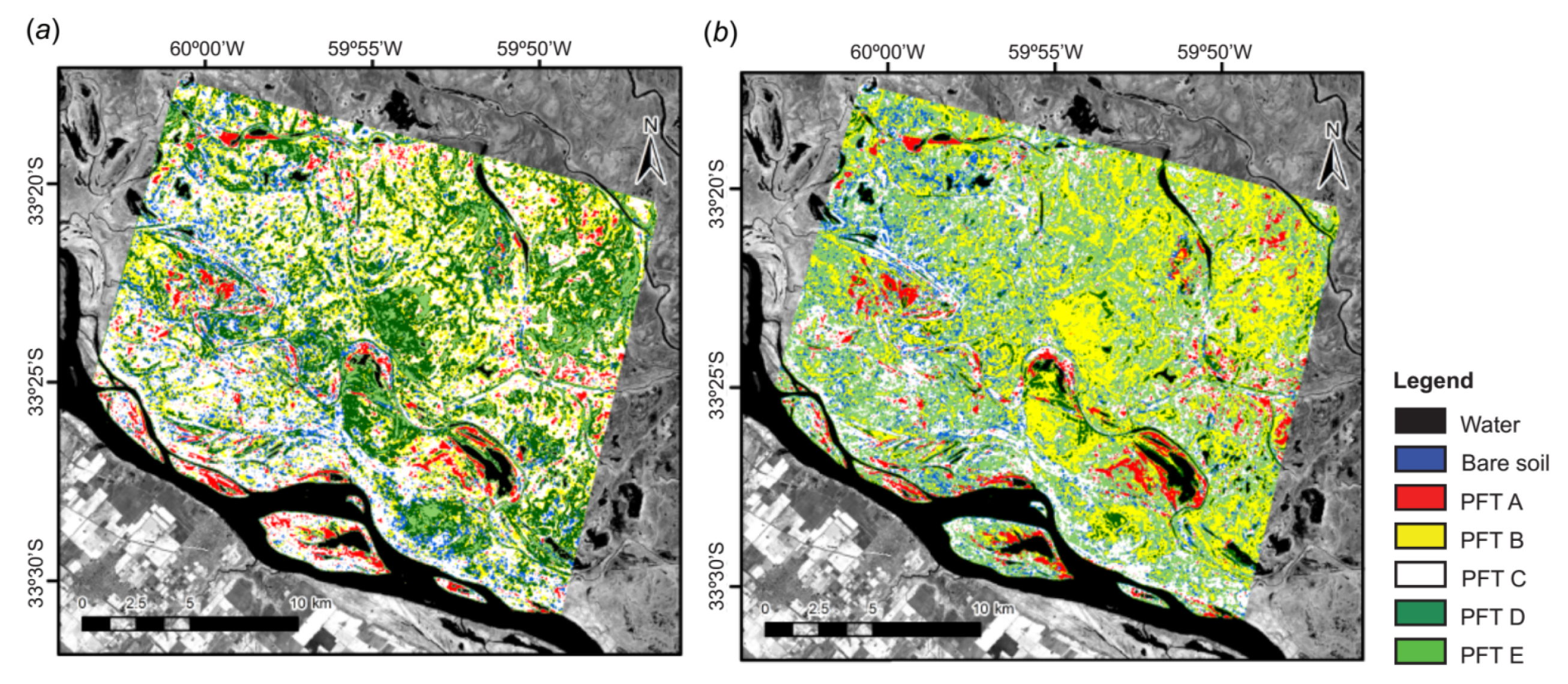
3.3. Unsupervised Wishart H/α and H/A/α Classifications

The H/α Wishart classifiers converged to eight classes by shifting most of the centroids of the segmented plane to areas with high H and intermediate α (Figure 4c,d). In both classifications, the centroid of one of the classes had very high α (α > 60°, dihedral reflectors, big ships). Thus, this class was excluded in further analyses. Next, the class with the lowest H and α was assigned to the open-water class. Among the remaining classes, the one with the lowest H (and low α) was assumed to belong to bare soil. The remaining classes were labeled as stated in Section 2.3.3 (Figure 4e,f). Both the bare soil and the PFT D (short grasslands, see Table 2) classes had lower α in the steep angle scene than in the shallow angle one.
In the shallow angle classification product, four classes had H > 0.90 and were provisionally assigned to PFT E, A, B and C (in increasing order of H) (Figure 4e). For these four classes with H > 0.90, a progressive classification procedure was followed by analyzing H/A/α subclasses, i.e., those classes obtained with the H/A/α classifier within each H/α class (see scheme in Figure 2). Within PFT B, five H/A/α subclasses occurred. The geographic location of one out of these H/A/α subclasses was coincident with field records of sites dominated by PFT A, whereas other H/A/α subclass was coincident with field records of sites dominated by PFT C. The remaining H/A/α classes were retained in PFT B class. Thus, PFT discrimination was slightly improved by reassigning these two subclasses. The number of reassigned pixels was a minority compared to the total pixels in PFT B class. None of the pixels of PFT A, E and C were reassigned according to the H/A/α subclasses. The second labeling procedure (i.e., maximizing the Kappa index when assigning classes obtained to information classes) was coincident with the labeling carried out by means of our a priori criteria.
In the steep angle classification product, only one class had a mean H higher than 0.90 (PFT C) (Figure 4f), so that the progressive classification on H/A/α planes was omitted. The two labeling procedures led to different results. Class assignment to information classes following the a priori criteria is shown in Figure 4d,f. Besides, Kappa index was maximized for this scene when pixels first assigned to PFT B were re-assigned to PFT E, and vice versa. This result suggests that our physical hypotheses on vegetation were contrary to the observed pattern for these two PFTs, at least for the steep incidence angle scene. Our a priori criteria could be misleading due to the difficulty to infer mean H and α values from biomass and non-quantitative vegetation structure data (distribution of biomass, degree of randomness in the canopy). In addition, the fact that our working hypothesis seems to be more accurate for the shallow incidence angle scene than for the steep one, is consistent with the general good performance of shallow incidence angle scenes for discriminating herbaceous wetland vegetation in the literature [11].

3.4. Comparison between Incidence Angles and Accuracy Assessment

The spatial pattern of PFT classes differed according to incidence angles (Figure 5a vs. Figure 5b). Both maps were quite homogeneous without much noise (i.e., zones of vegetation were identifiable). The zonation of vegetation is typical in wetland ecosystems, where abiotic constraints are important for plant community development, and has been described for the study area [18]. The classification products obtained with the shallow and the steep incidence angle scenes were coincident in 30.0% (a concordance of 17.8% in comparison with the randomly expected concordance, as estimated by the Kappa index). Water was almost equally classified in both scenes. Most of the differences between the resulting products arose for PFT E (tall grasslands), for which we identified a total area of 31 km2 in the shallow angle product and an area of 149 km2 in the steep angle one. Besides, 70.4% of the pixels assigned to PFT D in the shallow angle product were assigned to PFT B in the steep angle one, confounding short grasslands and short broadleaf marshes. In addition, much of the areas identified as PFT C in the shallow angle product were identified as PFT E in the steep angle one, and vice versa; confounding tall broadleaf marshes and tall grasslands. This mismatch between the maps suggests that broadleaf and graminoid herbs interact differently with the SAR signal depending on the incidence angle.
Accuracy was higher for the shallow incidence angle scene than for the steep one. On the one hand, the product obtained with the shallow incidence angle scene had an overall accuracy of 61.5% or of 52.4% excluding the water class (Table 3). The class with lowest commission error was PFT B, whereas the one with lowest omission error was PFT C (Table S1). PFT D and PFT E (short and tall grasslands, respectively) were confounded. Sixty percent of the pixels belonging to PFT E were omitted and assigned to other PFTs and to bare soil. The accuracy differed from the chance-adjusted expected accuracy and the Kappa index was 54.8% or 42.5% (including or not water class, respectively) (Table 3). In comparison with the Isodata classification on HH, HV and VV, the Wishart classifier improved the accuracy by 20.7% (including the water class) or by 34.2% (without the water class), in line with previous comparisons of the performance of Wishart classifications derived from quad-pol imagery and of classifiers based on standard linear dual-pol imagery [66]. Regarding the omission errors (Table S1), some of the pixels classified as open water in marsh areas might actually correspond to flooded vegetation. In areas of the Amazonas floodplain dominated by macrophytes, mirror reflection has been reported for emergent biomass (above water level) up to 200 g/m2, from which volume scattering starts increasing [13]. Thus, some the flooded areas of PFT D and E could be underestimated and assigned to the water class.
On the other hand, the product obtained with the steep incident angle scene had an overall accuracy of 46.2% or of 35.0% excluding the water class (Table 3). Kappa indexes were low and, when excluding the water class, the 95% confidence interval included the zero. High omission errors were observed for all the PFTs and were the highest for PFT E (Table S1). Optimum class labeling in terms of Kappa maximization improved the results and led to an overall accuracy of 53.3% and a Kappa index of 42.9%. Even with the Kappa maximization criterion, the accuracy was higher for the shallow incidence angle scene than for the steep one, being the former the more reliable product.
The results suggest that our hypotheses between PFT and SAR signal interactions were accurate only for the case of shallow incidence angles. In addition, our results were consistent with the reported preference of shallow incidence angle SAR signals for discriminating vegetation types and of steep incidence angle signals for detecting water below marsh vegetation and for flood monitoring [11,12]. In our study, at least two observations support this fact: in comparison to the shallow incidence angle scene, the steep one showed a higher density of pixels with low H and low α (Figure 4d vs. Figure 4c); and the centroids of classes PFT B and C featured lower H and α. The observed pattern can be explained by considering that steep SAR signal is less attenuated by vegetation layers and can interact to soil or water below the vegetation.
Regarding double-bounce scattering, the interaction mechanism seems to be more common for targets observed with high incidence angle scenes: pixels with medium H and high α in the shallow incidence angle scene showed low H and low α in the steep one. In the case of flooded herbaceous vegetation with low emergent biomass, a vertical incidence angle may diminish the probability of a first bounce in vegetation and a second one in the water (or vice versa), increasing the probability of reaching water. This observation is in marked contrast to what happens in forest environments, where for a given polarization and frequency, double-bounce scattering is more important in steep than in shallow incidence angles scenes [12,25,67].
In the Lower Paraná River floodplain, previous vegetation maps performed with optic data have overestimated the forest coverage at the expense of herbaceous wetlands [68]. Thus, the map obtained with the shallow incidence angle scene is a better start point than optical-derived maps for monitoring wetland vegetation in the floodplain. In the future, the study of SAR/optical fusion schemes will be considered. Our results suggest that most of the area was dominated by a ruderal strategy or an intermediate ruderal-competitor strategy (PFTs B, C and E; 58.7% of the total area or 63.8% excluding water). Ruderal plants are characterized by fast growth rate, short life span and high seed production, thus are favored by chronically disturbed but potentially productive environments [52]. The hydrological regime periodically disturbs the marsh areas, along with cattle activity. Ruderal plants can quickly regenerate between two ordinary flooding events, thus exploiting and nutrients brought by the river and taking advantage of resource opportunities. In addition, plant species with intermediate ruderalness-competitiveness may play a crucial role in vegetation adaptation to wetland states or in disturbance resistance. The fact that most of the floodplain seems to be covered by ruderal or intermediate ruderal-competitor plants gives to the environment a high ability to recover after disturbances and ordinary floods [69,70].

4. Conclusions

In this study, the ability of C-Band polarimetric data to monitor plant functional types in the Lower Paraná River floodplain was assessed. Although it is easier to perform a non-polarimetric analysis of the data, our results showed that analyzing the complex polarimetric information improves the resulting accuracy in comparison with the use of a multipolarization stack (HH, HV and VV). Moreover, the use of polarimetric decompositions facilitated the interpretation of the interaction mechanisms between the SAR signal and the scatterers. The analysis of the H/α and H/A/α spaces improved the previous knowledge about the response of herbaceous wetland vegetation in the Lower Paraná River floodplain, particularly with regard to the interpretation of classifications results. The analysis of the two images with different incidence angles allowed confirming an important result widespread in the literature: the backscattering measured at shallow incidence angles is more sensitive to herbaceous vegetation structure. Moreover, a conclusion of this study is that a priori hypotheses on the physical interaction between SAR signal and vegetation types should be dependent on the incidence angle. We conclude that using a C-Band shallow incidence angle scene is more accurate for the study of herbaceous PFTs in the Paraná River floodplain than using a steep incidence angle scene. To assess whether the accuracy of the classifications may be improved, other decompositions rather than the Cloude–Pottier may be addressed (e.g., [36,38,71,72]), as well as object-based schemes [73]. These approaches may include SAR/optical fusion schemes (e.g., [74]).
Taking into account the overall complexity of the landscape in the area, where herbaceous plants dominate, the shallow incidence angle product adds significant information while compared with previous available maps. The map obtained provides novel ecologically relevant information, suggesting that ruderal and ruderal-competitor broadleaf herbs dominate the floodplain. Mapping PFTs is not a common application in remote sensing yet, especially in wetlands, but it is a promising tool for assessing wetland functional features and for predicting vegetation responses to floods, anthropic impacts and climate changes in large floodplains. In the future, this approach can be used to assess changes in functional diversity or to evaluate how plant strategies respond to environmental changes.

Supplementary Materials

The following are available online at www.mdpi.com/2072-4292/8/3/174, Table S1: Error matrices of the Wishart classification products obtained with the RADARSAT-2 scenes. Overall accuracy and Kappa indexes are provided in Table 3.

Acknowledgments

RADARSAT-2 imagery was acquired through a project with the Canadian Space Agency. The work was funded by Comisión Nacional de Actividades Espaciales (AO SAOCOM N° 22) and by Agencia Nacional de Promoción Científica y Técnica (PICTO-CIN I N° 22, PICT 2014-0824). Part of the fieldwork was funded by Neotropical Grassland Conservancy. We thank four anonymous reviewers for their valuable comments on a previous version of the manuscript. We thank Nazar, J. for allowing field sampling in his farms and Bello family for their help during the surveys. Several people helped in fieldwork: Borro, M.; Schoo, M.; Varela, S.; Derguy, M.R.; Erario, M.S.; Falthauser, A.; Lanfiutti, M.; and Pacotti, V. We are also grateful to Salvia, M. for her help during SAR data processing.

Author Contributions

Natalia S. Morandeira led the writing and the other authors contributed significantly to the manuscript. Sampling design and fieldwork was conducted by Natalia S. Morandeira and Patricia Kandus. Pre-processing and classification of RADARSAT-2 imagery was conducted by Natalia S. Morandeira, Francisco Grings and Claudia Facchinetti.

Conflicts of Interest

The authors declare no conflict of interest.

References

  1. Junk, W.J. Current state of knowledge regarding South America wetlands and their future under global climate change. Aquat. Sci. 2012, 75, 113–131. [Google Scholar] [CrossRef]
  2. Baigún, C.R.M.M.; Puig, A.; Minotti, P.G.; Kandus, P.; Quintana, R.D.; Vicari, R.L.; Bó, R.F.; Oldani, N.O.; Nestler, J.A. Resource use in the Parana River Delta (Argentina): Moving away from an ecohydrological approach? Ecohydrol. Hydrobiol. 2008, 8, 245–262. [Google Scholar] [CrossRef]
  3. Junk, W.J.; An, S.; Finlayson, C.M.; Gopal, B.; Květ, J.; Mitchell, S.A.; Mitsch, W.J.; Robarts, R.D. Current state of knowledge regarding the world’s wetlands and their future under global climate change: A synthesis. Aquat. Sci. 2013, 75, 151–167. [Google Scholar] [CrossRef]
  4. Mertes, L.A.K.; Daniel, D.L.; Melack, J.M.; Nelson, B.; Martinelli, A.; Forsberg, B.R. Spatial patterns of hydrology, geomorphology, and vegetation on the floodplain of the Amazon River from a remote sensing perspective. Geomorphology 1995, 13, 215–232. [Google Scholar] [CrossRef]
  5. Novo, E.M.L.M.; Shimabukuro, Y.E. Identification and mapping of the Amazon habitats using a mixing model. Int. J. Remote Sens. 1997, 18, 663–670. [Google Scholar] [CrossRef]
  6. Salvia, M.M.; Karszenbaum, H.; Kandus, P.; Grings, F.M. Datos satelitales ópticos y de radar para el mapeo de ambientes en macrosistemas de humedal. Rev. Teledetec. 2009, 31, 35–51. [Google Scholar]
  7. Silva, T.S.F.; Costa, M.P.F.; Melack, J.M.; Novo, E.M.L.M. Remote sensing of aquatic vegetation: Theory and applications. Environ. Monit. Assess. 2008, 140, 131–145. [Google Scholar] [CrossRef] [PubMed]
  8. Hess, L.L.; Melack, J.M.; Novo, E.M.L.M.; Barbosa, C.C.F.; Gastil, M. Dual-season mapping of wetland inundation and vegetation for the central Amazon basin. Remote Sens. Environ. 2003, 87, 404–428. [Google Scholar] [CrossRef]
  9. Pope, K.O.; Rey-Benayas, J.M.; Paris, J.F. Radar remote sensing of forest and wetland ecosystems in the Central American tropics. Remote Sens. Environ. 1994, 48, 205–219. [Google Scholar] [CrossRef]
  10. Silva, T.S.F.; Costa, M.P.F.; Melack, J.M. Spatial and temporal variability of macrophyte cover and productivity in the eastern Amazon floodplain: a remote sensing approach. Remote Sens. Environ. 2010, 114, 1998–2010. [Google Scholar] [CrossRef]
  11. Henderson, F.M.; Lewis, A.J. Radar detection of wetland ecosystems: A review. Int. J. Remote Sens. 2008, 29, 5809–5835. [Google Scholar] [CrossRef]
  12. Hess, L.L.; Melack, J.M.; Simonett, D. Radar detection of flooding beneath the forest canopy: A review. Int. J. Remote Sens. 1990, 11, 1313–1325. [Google Scholar] [CrossRef]
  13. Costa, M.P.F.; Niemann, O.; Novo, E.M.L.M.; Ahern, F. Biophysical properties and mapping of aquatic vegetation during the hydrological cycle of the Amazon floodplain using JERS-1 and Radarsat. Int. J. Remote Sens. 2002, 23, 1401–1426. [Google Scholar] [CrossRef]
  14. Novo, E.M.L.M.; Costa, M.P.F.; Mantovani, J.E.; Lima, I.B.T. Relationship between macrophyte stand variables and radar backscatter at L and C band, Tucuruí reservoir, Brazil. Int. J. Remote Sens. 2002, 23, 1241–1260. [Google Scholar] [CrossRef]
  15. Grings, F.M.; Ferrazzoli, P.; Karszenbaum, H.; Salvia, M.M.; Kandus, P.; Jacobo-Berlles, J.C.; Perna, P. Model investigation about the potential of C band SAR in herbaceous wetlands flood monitoring. Int. J. Remote Sens. 2008, 29, 5361–5372. [Google Scholar] [CrossRef]
  16. Kandus, P.; Karszenbaum, H.; Pultz, T.; Parmuchi, M.G.; Bava, J. Influence of flood conditions and vegetation status on the radar backscatter of wetland ecosystems. Can. J. Remote Sens. 2001, 27, 651–662. [Google Scholar] [CrossRef]
  17. Parmuchi, M.G.; Karszenbaum, H.; Kandus, P. Mapping wetlands using multi-temporal RADARSAT-1 data and a decision-based classifier. Can. J. Remote Sens. 2002, 28, 175–186. [Google Scholar] [CrossRef]
  18. Morandeira, N.S.; Kandus, P. Multi-scale analysis of environmental constraints on macrophyte distribution, floristic groups and plant diversity in the Lower Paraná River floodplain. Aquat. Bot. 2015, 123, 13–25. [Google Scholar] [CrossRef]
  19. Kandus, P.; Malvárez, A.I.; Madanes, N. Estudio de las comunidades de plantas herbáceas de las islas bonaerenses del Bajo Delta del Río Paraná (Argentina). Darwiniana 2003, 41, 1–16. [Google Scholar]
  20. Ramsey III, E. Radar remote sensing of wetlands. In Remote Sensing Change Detection: Environmental Monitoring Methods and Applications; Lunetta, R., Elviidge, C., Eds.; Ann Harbor Press: Chelsea, MA, USA, 1998; pp. 211–243. [Google Scholar]
  21. Kasischke, E.S.; Melack, J.M.; Dobson, M.C. The use of imaging radars for ecological applications—A review. Remote Sens. Environ. 1997, 59, 141–156. [Google Scholar] [CrossRef]
  22. Schmullius, C.C.; Evans, D.L. Tabular summary of SIR-C/X-SAR results: Synthetic Aperture Radar frequency and polarization requirements for applications in ecology and hydrology. In Proceedings of the 1997 IEEE International Geoscience and Remote Sensing Symposium, Suntec City, Singapore, 3–8 August 1997; pp. 1734–1736.
  23. Touzi, R.; Deschamps, A.; Rother, G. Phase of target scattering for wetland characterization using polarimetric C-Band SAR. IEEE Trans. Geosci. Remote Sens. 2009, 47, 3241–3261. [Google Scholar] [CrossRef]
  24. Hess, L.L.; Melack, J.M.; Filoso, S.; Wang, Y. Delineation of inundated area and vegetation along the Amazon Floodplain with the SIR-C Synthetic Aperture Radar. IEEE Trans. Geosci. Remote Sens. 1995, 33, 896–904. [Google Scholar] [CrossRef]
  25. Pope, K.O.; Rejmankova, E.; Woodruff, R. Detecting seasonal flooding cycles in marshes of the Yucatan Peninsula with SIR-C polarimetric radar imagery. Remote Sens. Environ. 1997, 4257, 157–166. [Google Scholar] [CrossRef]
  26. Sokol, J.; NcNairn, H.; Pultz, T.J. Case studies demonstrating the hydrological applications of C-band multipolarized and polarimetric SAR. Can. J. Remote Sens. 2004, 30, 470–483. [Google Scholar] [CrossRef]
  27. Ferrazzoli, P.; Guerriero, L.; Schiavon, G. Experimental and model investigation on radar classification capability. IEEE Trans. Geosci. Remote Sens. 1999, 37, 960–968. [Google Scholar] [CrossRef]
  28. Kim, Y.; van Zyl, J. Comparison of forest parameter estimation techniques using SAR data. In Proceedings of the 2001 IEEE International Geoscience and Remote Sensing Symposium, Sydney, Australia, 9–13 July 2001; pp. 1395–1397.
  29. Marti-Cardona, B.; Lopez-Martinez, C.; Dolz-Ripolles, J.; Bladè-Castellet, E. ASAR polarimetric, multi-incidence angle and multitemporal characterization of Doñana wetlands for flood extent monitoring. Remote Sens. Environ. 2010, 114, 2802–2815. [Google Scholar] [CrossRef]
  30. Turkar, V.; Rao, Y.S. Analysis of multi-frequency polarimetric SAR data using different classification techniques. In Proceedings of the 2011 International Conference and Workshop on Emerging Trends in Technology (ICWET), Mumbai, India, 25–26 February 2011; pp. 53–60.
  31. Touzi, R.; Deschamps, A.; Rother, G. Wetland characterization using polarimetric RADARSAT-2 capability. Can. J. Remote Sens. 2007, 33, S56–S67. [Google Scholar] [CrossRef]
  32. Sartori, L.R.; Imai, N.N.; Mura, J.C.; Novo, E.M.L.M.; Silva, T.S.F. Mapping macrophyte species in the Amazon floodplain wetlands using fully polarimetric ALOS/PALSAR data. IEEE Trans. Geosci. Remote Sens. 2011, 49, 4717–4728. [Google Scholar] [CrossRef]
  33. Brisco, B.; Li, K.; Tedford, B.; Charbonneau, F.; Yun, S.; Murnaghan, K. Compact polarimetry assessment for rice and wetland mapping. Int. J. Remote Sens. 2013, 34, 1949–1964. [Google Scholar] [CrossRef]
  34. Storie, J.; Lawson, A.; Storie, C. Using L-band SAR images to map coastal wetlands. In Proceedings of the 2012 IEEE International Geoscience and Remote Sensing Symposium, Munich, Germany, 22–27 July 2012; pp. 757–759.
  35. Pottier, E.; Marechal, C.; Allain-Bailhache, S.; Meric, S.; Hubert-Moy, L.; Corgne, S. On the use of fully polarimetric RADARSAT-2 time-series datasets for delineating and monitoring the seasonal dynamics of wetland ecosystem. In Proceedings of the 2012 IEEE International Geoscience and Remote Sensing Symposium, Munich, Germany, 22–27 July 2012; pp. 107–110.
  36. Hong, S.-H.; Kim, H.-O.; Wdowinski, S.; Feliciano, E. Evaluation of polarimetric SAR decomposition for classifying wetland vegetation types. Remote Sens. 2015, 7, 8563–8585. [Google Scholar] [CrossRef]
  37. Furtado, L.F.D.A.; Silva, T.S.F.; Novo, E.M.L.M. Dual-season and full-polarimetric C band SAR assessment for vegetation mapping in the Amazon várzea wetlands. Remote Sens. Environ. 2016, 174, 212–222. [Google Scholar] [CrossRef]
  38. Gosselin, G.; Touzi, R.; Cavayas, F. Polarimetric Radarsat-2 wetland classification using the Touzi decomposition: case of the Lac Saint-Pierre Ramsar wetland. Can. J. Remote Sens. 2014, 39, 491–506. [Google Scholar] [CrossRef]
  39. Van Beijma, S.; Comber, A.; Lamb, A. Random forest classification of salt marsh vegetation habitats using quad-polarimetric airborne SAR, elevation and optical RS data. Remote Sens. Environ. 2014, 149, 118–129. [Google Scholar] [CrossRef]
  40. Díaz, S.; Cabido, M. Vive la différence: Plant functional diversity matters to ecosystem processes. Trends Ecol. Evol. 2001, 16, 646–655. [Google Scholar] [CrossRef]
  41. Ustin, S.L.; Gamon, J.A. Remote sensing of plant functional types. New Phytol. 2010, 186, 795–816. [Google Scholar] [CrossRef] [PubMed]
  42. Hooper, D.U.; Solan, M.; Symstad, A.; Díaz, S.; Gessner, M.O.; Buchmann, N.; Degrange, V.; Grime, P.; Hulot, F.; Mermillod-Blondin, F.; et al. Species diversity, functional diversity, and ecosystem functioning. In Biodiversity and Ecosystem Functioning. SYNTHESIS and Perspectives; Loreau, M., Naeem, S., Inchausti, P., Eds.; Oxford University Press: Oxford, UK, 2002; pp. 195–281. [Google Scholar]
  43. Díaz, S.; Lavorel, S.; de Bello, F.; Quétier, F.; Grigulis, K.; Robson, T.M. Incorporating plant functional diversity effects in ecosystem service assessments. Proc. Natl. Acad. Sci. USA 2007, 104, 20684–20689. [Google Scholar] [CrossRef] [PubMed]
  44. De Bello, F.; Lavorel, S.; Díaz, S.; Harrington, R.; Cornelissen, J.H.C.; Bardgett, R.D.; Berg, M.P.; Cipriotti, P.; Feld, C.K.; Hering, D.; et al. Towards an assessment of multiple ecosystem processes and services via functional traits. Biodivers. Conserv. 2010, 19, 2873–2893. [Google Scholar] [CrossRef]
  45. Bornette, G.; Tabacchi, E.; Hupp, C.; Puijalon, S.; Rostan, J.C. A model of plant strategies in fluvial hydrosystems. Freshw. Biol. 2008, 53, 1692–1705. [Google Scholar] [CrossRef]
  46. Enrique, C. Relevamiento y Caracterización Florística y Espectral de los Bosques de la Región del Delta del Paraná a Partir de Imágenes Satelitales. Bachelor’s Thesis, Biological Sciences, FCEN-UBA, Buenos Aires, Argentina, December 2009. [Google Scholar]
  47. Salvia, M.M.; Grings, F.M.; Barraza, V.; Perna, P.; Karszenbaum, H.; Ferrazzoli, P. Active and passive microwave systems in the assessment of flooded area fraction and mean water level in the Paraná River floodplain. In Proceedings of the 12th Specialist Meeting on Microwave Radiometry and Remote Sensing of the Environment (MicroRad), Frascati, Italia, 5–9 March 2012; pp. 1–4.
  48. European Space Agency PolSARpro. V. 4.2. Available online: http://earth.eo.esa.int/polsarpro/ (accessed on 1 November 2013).
  49. Alaska Satellite Facility ASF Map Ready v. 3.0.6. Available online: https://www.asf.alaska.edu/data-tools/mapready/ (accessed on 1 November 2013).
  50. Lee, J.-S. Speckle supression and analysis for Synthetic Aperture Radar images. Opt. Eng. 1986, 25, 255636. [Google Scholar] [CrossRef]
  51. Lee, J.-S.; Pottier, E. Polarimetric Radar Imaging: From Basics to Applications; CRC Press: Boca Raton, FL, USA, 2009; p. 398. [Google Scholar]
  52. Menges, E.; Waller, D. Plant strategies in relation to elevation and light in floodplain herbs. Am. Nat. 1983, 122, 454–473. [Google Scholar] [CrossRef]
  53. Grime, J.P. Evidence for the existence of three primary strategies in plants and its relevance to ecological and evolutionary theory. Am. Nat. 1977, 111, 1169–1194. [Google Scholar] [CrossRef]
  54. Wheeler, B. lmPerm: Permutation Tests for Linear Models. R Package Version 1.1–2. Available online: http://cran.r-project.org/package=lmPerm (accessed on 1 November 2013).
  55. R Core Team R: A language and Environment for Statistical Computing. R Foundation for Statistical Computing, Vienna, Austria. 2014. Available online: http://www.r-project.org/ (accessed on 1 July 2014).
  56. Cloude, S.R.; Pottier, E. An entropy based classification scheme for land applications of polarimetric SAR. IEEE Trans. Geosci. Remote Sens. 1997, 35, 68–78. [Google Scholar] [CrossRef]
  57. Pottier, E. Radar target decomposition theorems and unsupervized classification of full polarimetric data. In Proceedings of the 1994 IEEE International Geoscience and Remote Sensing Symposium, Pasadena, CA, USA, 8–12 August 1994; pp. 1139–1141.
  58. Lee, J.-S.; Grunes, M.R.; Ainsworth, T.L.; Du, L.-J.; Schuler, D.L.; Cloude, S.R. Unsupervised classification using polarimetric decomposition and the complex Wishart classifier. IEEE Trans. Geosci. Remote Sens. 1999, 37, 2249–2258. [Google Scholar]
  59. Pottier, E.; Lee, J.-S. Application of the “H/A/α” polarimetric decomposition theorem for unsupervised classification of fully polarimetric SAR data based on the Wishart distribution. SAR Workshop 2000, 1, 335–340. [Google Scholar]
  60. Grings, F.M.; Ferrazzoli, P.; Karszenbaum, H.; Tiffenberg, J.; Kandus, P.; Guerriero, L.; Jacobo-Berlles, J.C. Modeling temporal evolution of Junco marshes radar signatures. IEEE Trans. Geosci. Remote Sens. 2005, 43, 2238–2245. [Google Scholar] [CrossRef]
  61. Cohen, J.A. A coefficient of agreement for nominal scales. Educ. Psychol. Meas. 1960, 20, 213–220. [Google Scholar] [CrossRef]
  62. Pontius, R.G., Jr.; Millones, M. Death to Kappa: Birth of quantity disagreement and allocation disagreement for accuracy assessment. Int. J. Remote Sens. 2011, 32, 4407–4429. [Google Scholar] [CrossRef]
  63. Ball, G.H.; Hall, D.J. ISODATA, A Novel Method of Data Analysis and Pattern Classification; Stanford Research Institute: Menlo Park, CA, USA, 1995; p. 61. [Google Scholar]
  64. Dickinson, C.; Siqueira, P.; Clewley, D.; Lucas, R. Classification of forest composition using polarimetric decomposition in multiple landscapes. Remote Sens. Environ. 2013, 131, 206–214. [Google Scholar] [CrossRef]
  65. Ferro-Famil, L.; Pottier, E.; Lee, J.-S. Unsupervised classification of multifrequency and fully polarimetric SAR images based on the H/A/Alpha-Wishart classifier. IEEE Trans. Geosci. Remote Sens. 2001, 39, 2332–2342. [Google Scholar] [CrossRef]
  66. Ainsworth, T.L.; Kelly, J.P.; Lee, J.S. Classification comparisons between dual-pol, compact polarimetric and quad-pol SAR imagery. ISPRS J. Photogramm. Remote Sens. 2009, 64, 464–471. [Google Scholar] [CrossRef]
  67. Wang, Y.; Hess, L.L.; Filoso, S.; Melack, J.M. Understanding the radar backscattering from flooded and nonflooded Amazonian Forests: results from canopy backscatter modeling. Remote Sens. Environ. 1995, 54, 324–332. [Google Scholar] [CrossRef]
  68. Salvia, M.M. Aporte de la teledetección al estudio del funcionamiento del macrosistema Delta del Paraná: Análisis de series de tiempo y eventos extremos. Ph.D Thesis, FCEN-UBA, Buenos Aires, Argentina, 11 June 2010. [Google Scholar]
  69. Franceschi, E.A.; Torres, P.S.; Prado, D.E.; Lewis, J.P. Disturbance, sucession and stability: a ten year study of temporal variation of species composition after a catastrophic flood in the river Paraná, Argentina. Community Ecol. 2000, 1, 205–214. [Google Scholar] [CrossRef]
  70. Franceschi, E.A.; Torres, P.S.; Lewis, J.P. Recovery and stability of Paraná river floodplain grasslands twenty years after a catastrophic flood. Community Ecol. 2005. [Google Scholar] [CrossRef]
  71. Hong, S.-H.; Wdowinski, S. Double-bounce component in cross-polarimetric SAR from a new scattering target secomposition. IEEE Trans. Geosci. Remote Sens. 2014, 52, 3039–3051. [Google Scholar] [CrossRef]
  72. Yajima, Y.; Yamaguchi, Y.; Sato, R.; Yamada, H.; Boerner, W.-M. POLSAR image analysis of wetlands using a modified four-component scattering power decomposition. IEEE Trans. Geosci. Remote Sens. 2008, 46, 1667–1673. [Google Scholar] [CrossRef]
  73. Blaschke, T.; Hay, G.J.; Kelly, M.; Lang, S.; Hofmann, P.; Addink, E.; Feitosa, R.Q.; van Der Meer, F.; van Der Werff, H.; van Coillie, F.; et al. Geographic object-based image analysis—Towards a new paradigm. ISPRS J. Photogramm. Remote Sens. 2014, 87, 180–191. [Google Scholar] [CrossRef] [PubMed]
  74. Ullmann, T.; Schmitt, A.; Roth, A.; Duffe, J.; Dech, S.; Hubberten, H.-W.; Baumhauer, R. Land cover characterization and classification of Arctic Tundra environments by means of Polarized Synthetic Aperture X- and C-Band Radar (PolSAR) and Landsat 8 multispectral imagery—Richards Island, Canada. Remote Sens. 2014, 6, 8565–8593. [Google Scholar] [CrossRef]
Figure 1. Study area and acquired scenes: (a) Location of the Lower Paraná River floodplain in Del Plata Basin in South America; (b) Lower Paraná River floodplain, from Diamante city to the Del Plata River; (c) Pauli representation of the shallow incidence angle scene (beam FQ24, see Table 1) of 30 January 2011; and (d) Pauli representation of the steep incidence angle scene (beam FQ08, see Table 1) of 2 February 2011. In both (c) and (d), colors were assigned as follows: Red = |HH − VV|; Green = |HV + VH| = 2|HV|; Blue = |HH – VV|. The background image shows the near infrared band from a Landsat 5TM scene of 1 February 2011.
Remotesensing 08 00174 g001
Figure 2. Methodological scheme for pre-processing and processing the scenes.
Remotesensing 08 00174 g002
Figure 3. Backscattering of the field samples for each of the PFTs (see Table 2 for a description of their features): (a) shallow incidence angle scene, HH polarization; (b) steep incidence angle scene, HH polarization; (c) shallow incidence angle scene, HV polarization; (d) steep incidence angle scene, HV polarization; (e) shallow incidence angle scene, VV polarization; and (f) steep incidence angle scene, VV polarization. In each figure, the water class is plotted in a different scale than that of the bare soil and Plant Functional Types (PFT) classes. In the boxplots, boxes show the medians (thick line) and the 1st and 3rd quartiles (limits of the boxes); whiskers show the maximum and minimum values; outliers were omitted for clarity. The letters onto the boxplots represent significant differences in the backscattering coefficients (ANOVA tests, followed by Tukey comparisons) at 0.01 significance level.
Remotesensing 08 00174 g003
Figure 4. Cloude–Pottier H/α segmentations and relocation of the centroids after the H/α Wishart unsupervised classifications: (a) shallow incidence angle scene, segmented image; (b) steep incidence angle scene, segmented image; (c) shallow incidence angle scene, density of pixels in the H/α plane; (d) steep incidence angle scene, density of pixels in the H/α plane; (e) shallow incidence angle scene, detail of the centroids assigned to bare soil and plant functional types (PFTs) classes (H > 0.80 and α > 0.36); (f) steep incidence angle scene, detail of the centroids assigned to bare soil and PFTs classes (H > 0.80 and α > 0.36). In both (a) and (b), the background image shows the near infrared band from a Landsat 5TM scene of 1 February 2011. In (c) and (d), the H/α planes were divided in nine zones and the centroids of the classes obtained with the Wishart classifier are shown; DR stands for “dihedral reflector” and W stands for “water”. In (e) and (f), BS stands for “bare soil” and the letters A–D indicate the corresponding PFT. Class labeling followed a priori criteria (see Section 2.3.3) and was a working hypothesis assessed with field data (see Section 3.4).
Remotesensing 08 00174 g004
Figure 5. Products of the Wishart unsupervised classifications. (a) Shallow incidence angle scene (beam FQ24, see Table 2) of 30 January 2011; (b) Steep incidence angle scene (beam FQ08, see Table 2) of 2 February 2011. PFT stands for “plant functional type”. For details on the classes, see Table 1. Maps correspond to the a priori labeling criteria.
Remotesensing 08 00174 g005
Table 1. Acquired RADARSAT-2 scenes. Nominal pixel spacing, resolution, nominal scene size and number of looks are indicated in range and azimuth.
SceneShallow Incidence AngleSteep Incidence Angle
Date30 January 20112 February 2011
Beam ModeFine Quad-PolFine Quad-Pol
Polarization OptionsHH, VV, HV, VHHH, VV, HV, VH
ProductSLCSLC
BeamFQ24FQ08
Near incidence angle42.8°26.9°
Far incidence angle44.1°28.7°
Near resolution7.7 m11.5 m
Far resolution7.5 m10.8 m
Nominal pixel spacing4.7 m × 5.1 m4.7 m × 5.1 m
Resolution5.2 m × 7.6 m5.2 m × 7.6 m
Nominal scene size25 km × 25 km25 km × 25 km
Number of looks1 × 11 × 1
Table 2. Featur of the plant functional types (PFTs) identified in the study area.
PFTABCDE
Morphoecological typeEquisetoid herbsBroadleaf herbsGraminoid herbs
PhysiognomyBulrush marshesShort broadleaf marshesTall broadleaf marshesShort grasslands and grass marshesTall grasslands and grass marshes
Plant height140–250 cm<150 cm (most: <80 cm)150–250 cm.<50 cm50–150 cm
Aboveground green biomass290–2330 g·m−2250–1320 g·m−2370–1390 g·m−2110–620 g·m−2100–3340 g·m−2
Aboveground green biomass distributionBiomass distributed in vertically oriented cylindrical stems.Biomass distributed in broadleaf leaves. Generally, few leaves with large leaf areas. Weak stems, often hollow stems or with aerenchyma tissues. Both decumbent and erect plants. Biomass amount does not depend on plant height.Biomass distributed in broadleaf leaves and stems. Generally, abundant leaves with small leaf areas. Stronger stems than in PFT B, often not hollow. Erect plants. Biomass amount increases with plant height.Biomass distributed in leaf blades. Generally, not hollow stems. Generally, decumbent plants.Biomass distributed in leaf blades and leaf sheaths. Either hollow or not hollow stems. Generally, erect plants.
Functional featuresStrong competitors growing in low topographic positions, in generally flooded sites. Clonal and perennial. Rapid regeneration. Tall plants with large seed size, low specific photosynthetic area, low leaf N. C3 plants.Ruderal plants growing in low topographic positions, in generally flooded or soil-saturated sites with high soil fertility (usually high N). Clonal and perennial. Medium specific leaf area, medium to high leaf nitrogen. C3 plants.Intermediate ruderal-competitor plants, growing in high (non-flooded sites; e.g., Baccharis salicifolia, Conyza bonariensis) or in low topographic positions (flooded sites; e.g., Ludwigia cf. peruviana). Annual and clonal plants. Medium specific leaf area, medium to high leaf N. C3 plants.Stress-tolerant species (both for salinity or dry conditions) or ruderal species, growing in high or medium topographic positions. Small leaf thickness, low leaf N and chlorophyll content. Mostly C4 plantsRuderal plants (or tolerant to salinity stress, Leptochloa fusca), growing in low or medium topographic positions. Either annual plants or clonal perennial plants. Both C3 and C4 plants.
SpeciesSchoenoplectus californicus, Cyperus giganteus.Sagittaria montevidensis, Eclipta prostrata, Enydra anagallis, Oplismenopsis najada, Polygonum acuminatum, Ludwigia cf. peruviana.Baccharis salicifolia, Conyza bonariensis, Polygonum acuminatum, Ludwigia cf. peruviana.Cynodon dactylon, Paspalum vaginatum, Echinochloa helodes, Echinochloa polystachya var. spectabilis.Panicum elephantipes, Hymenachne pernambucense, Echinochloa crus-gallis, Bolboschoenus robustus, Leptochloa fusca.
No.sites dominated894810
Predicted contribution of the scattering mechanismsVolumeMediumMediumHighLowMedium-High
SurfaceLow-NullLow-NullLow-NullMedium-HighLow-Null
Double-bounceMedium-HighLow-NullLowLow-NullLow
Table 3. Accuracy assessment of the classification products obtained with the RADARSAT-2 scenes. For the shallow incidence angle scene, the two class labeling procedures led to the same result, whereas for the steep incidence angle scene the results differed if the a priori labeling criteria were used or the Kappa index was maximized.
SceneShallow Incidence AngleSteep Incidence Angle
Class labelingA priori criteria and Maximizing KappaA priori criteriaMaximizing Kappa
Open-water classIncludedNot includedIncludedNot includedIncludedNot included
Overall accuracy (%)61.552.446.23553.342.9
Kappa index (%)54.842.529.49.745.129.6
Kappa 95% confidence interval (%)39.2–70.324.2–60.713.6–45.10.0–26.028.9–61.211.1–48.0
Improvement with regard to multipolarization Isodata classification (%)20.734.28.216.924.87.5

