
Effects of Urbanization and Seasonal Cycle on the Surface Urban Heat Island Patterns in the Coastal Growing Cities: A Case Study of Casablanca, Morocco


Abstract
:
1. Introduction
2. Study Area and Data
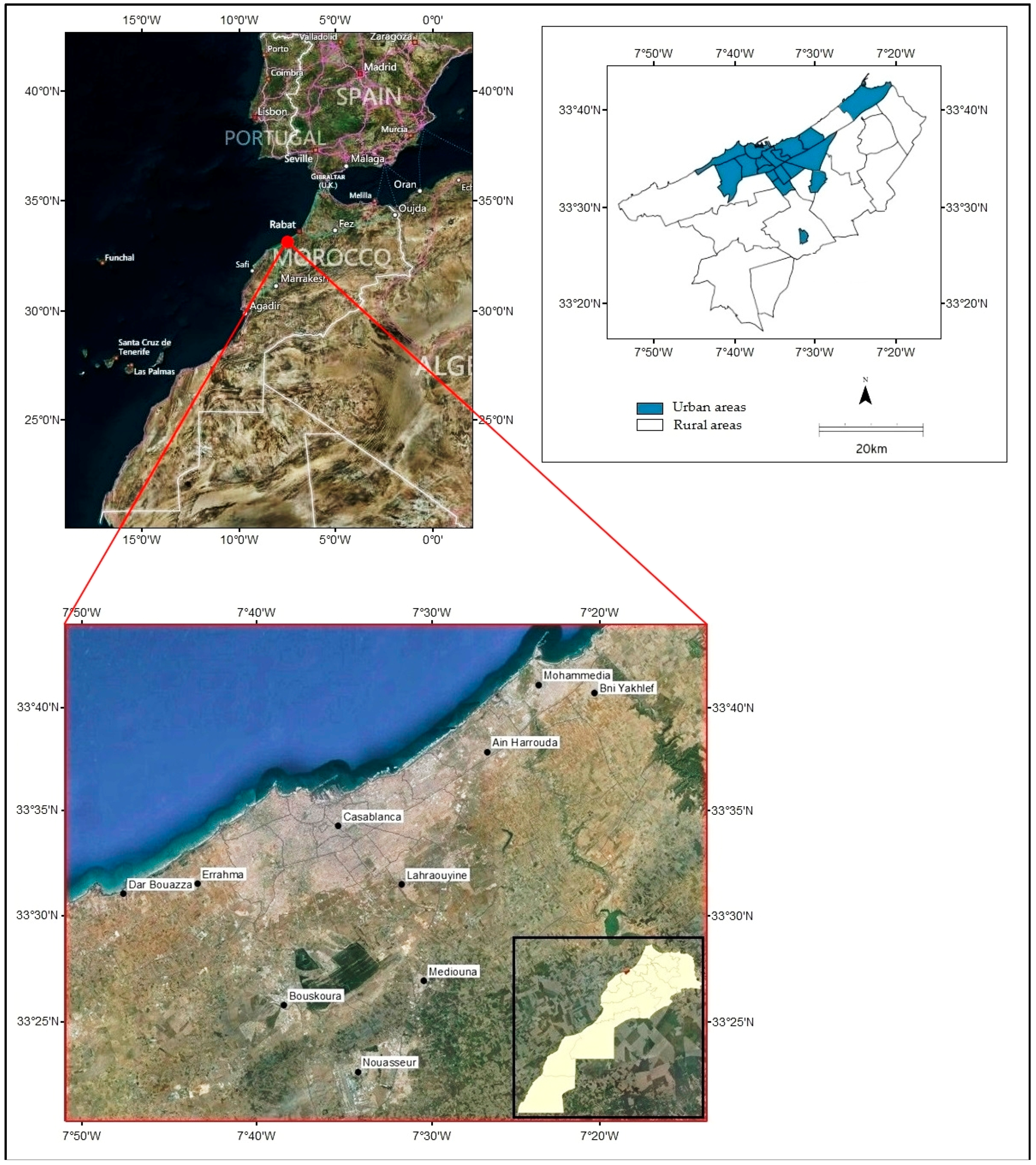
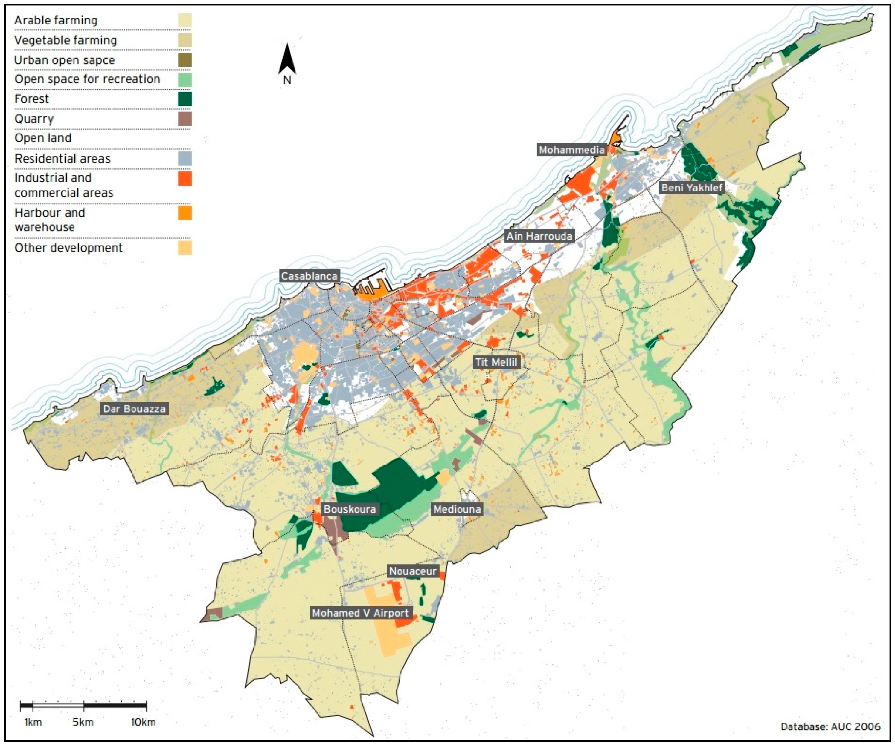
2.1. Study Area
2.2. Data Used
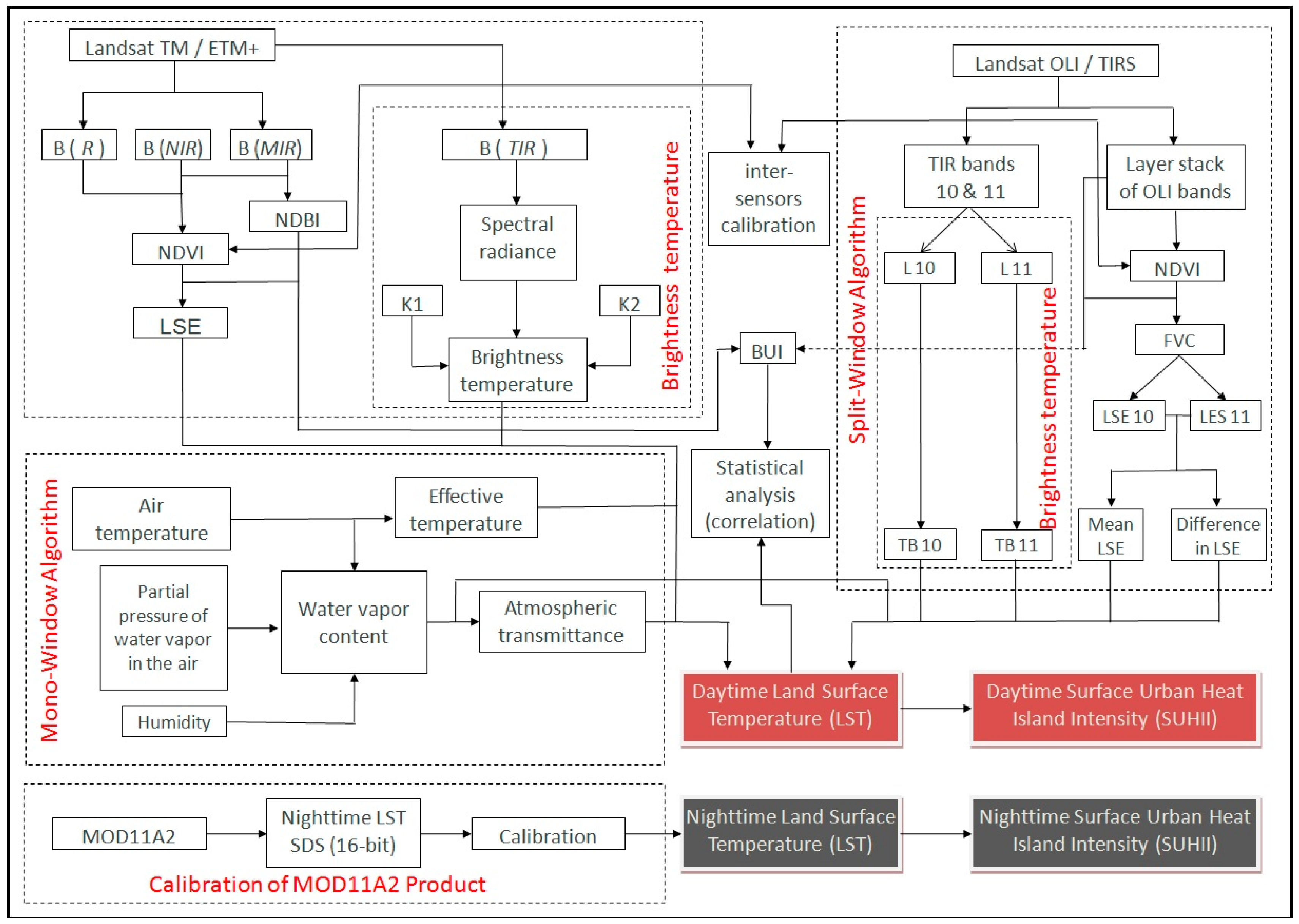
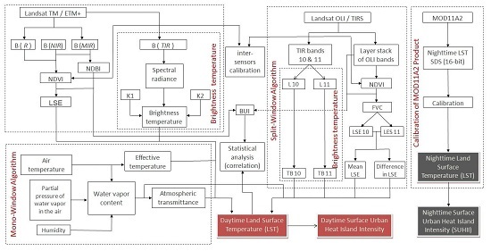
3. Methodology
3.1. Data Preparation
3.2. Calculation of NDVI
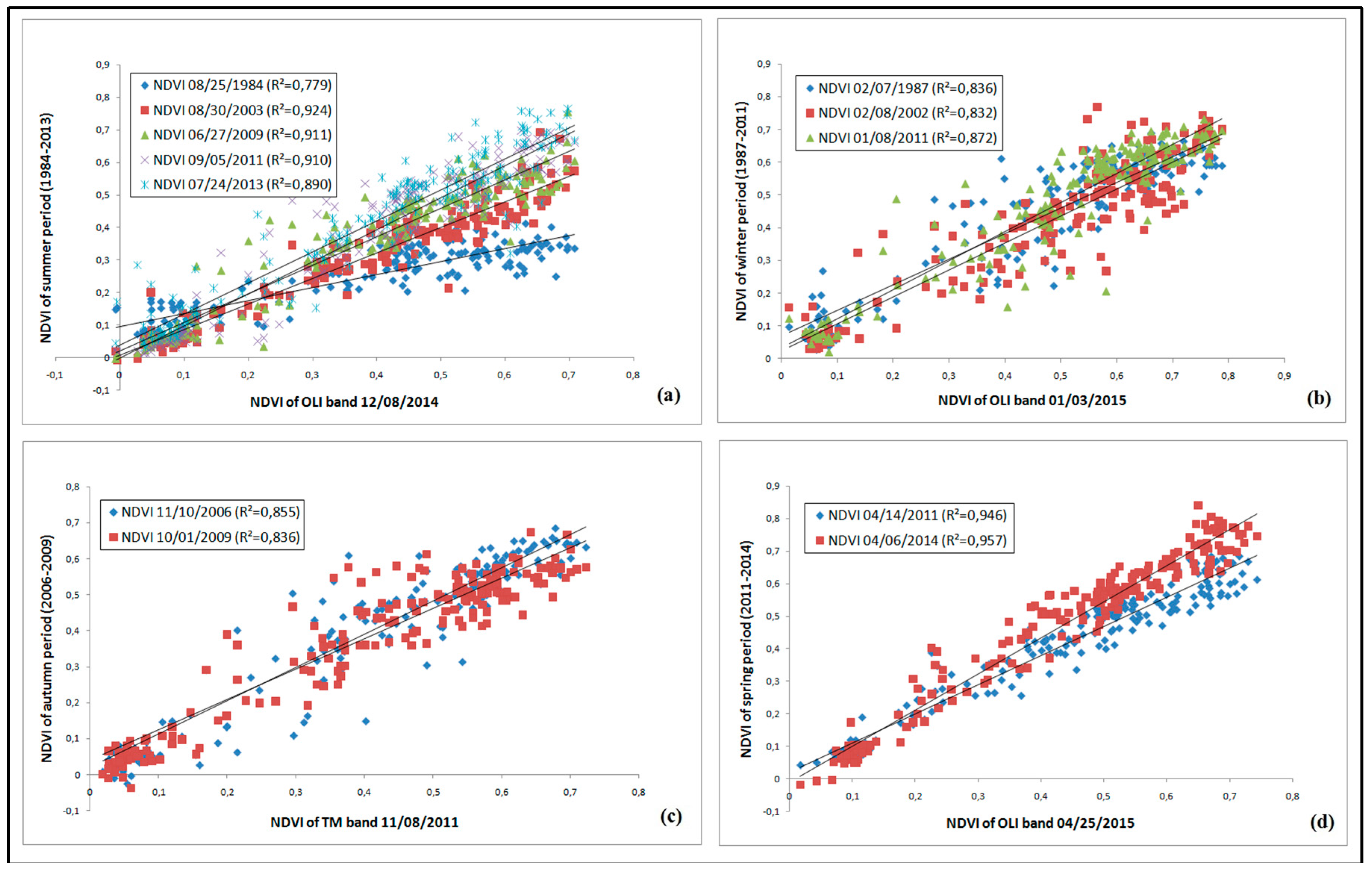
3.3. Inter-Calibration of Data
3.4. Retrieval of LSE
3.5. Retrieval of Land Surface Temperature
- Ts: Land surface temperature in Kelvin;
- c0 to c6: Split-Window coefficient [90];
- T10 and T11: At-sensor brightness temperature at band 10 and 11;
- ε: Mean of land surface emissivity of band 10 and 11;
- ∆ε: Difference between land surface emissivity of band 10 and band 11;
- ω: Atmospheric water vapor content.
3.6. Calculation of SUHII
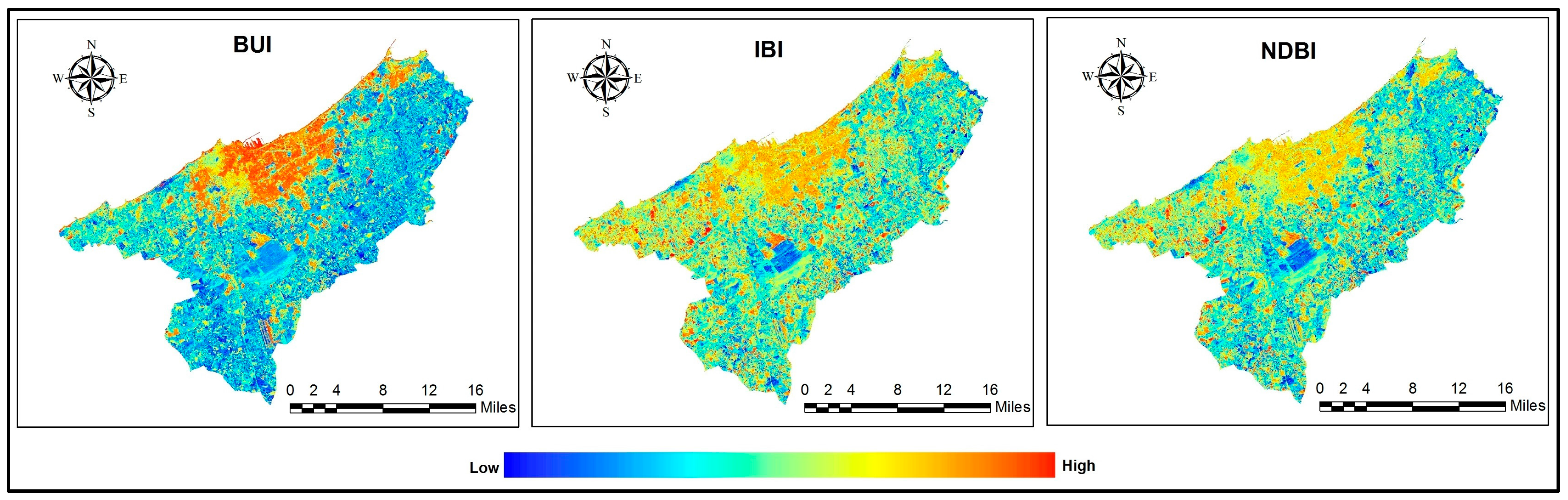
3.7. Calculation of Built-Up Land Information
4. Results
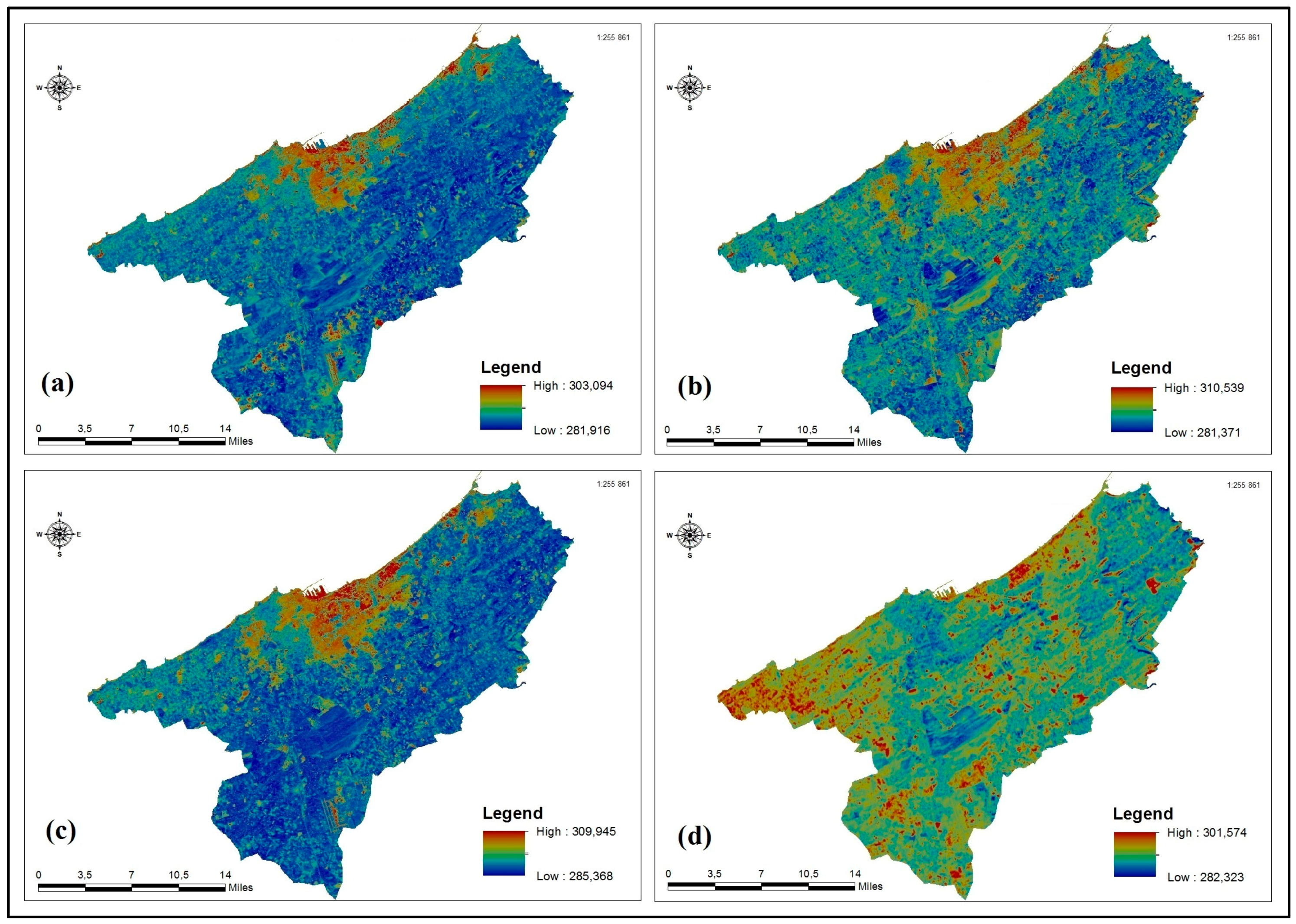
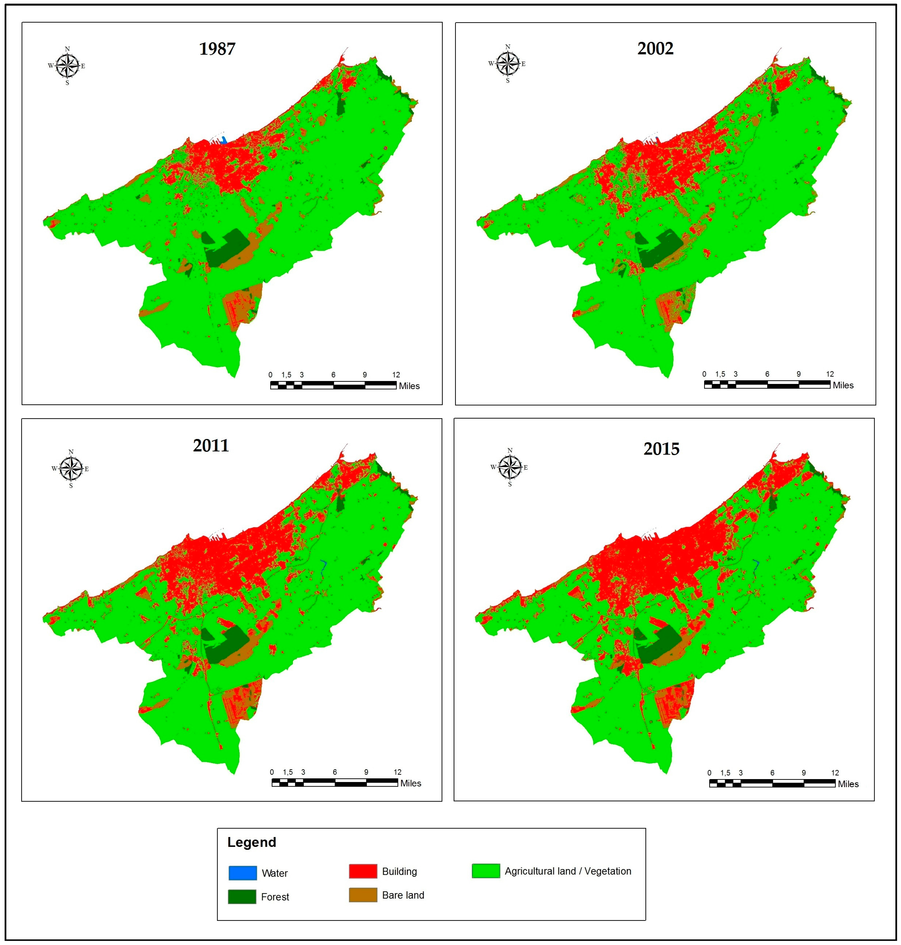
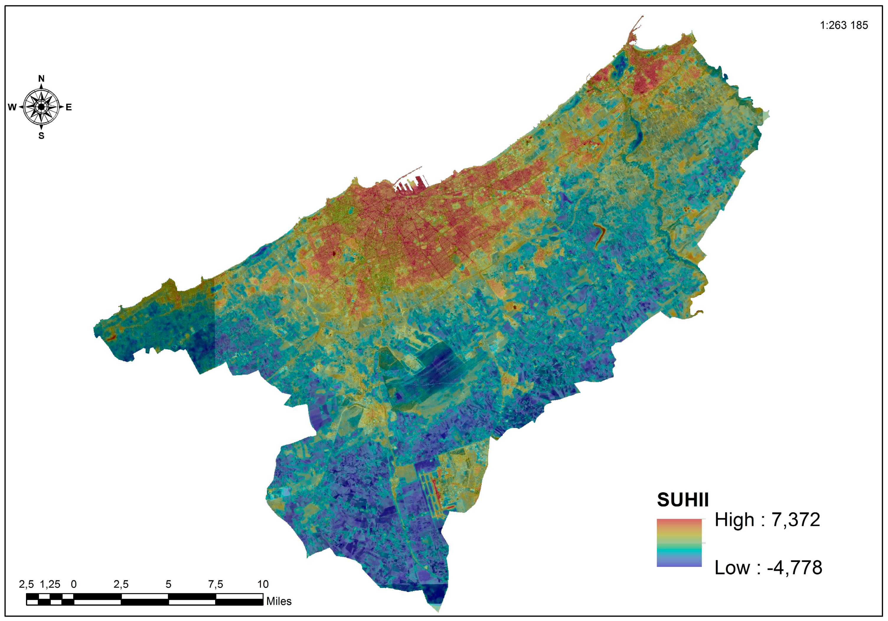
4.1. Spatial Distribution of LST in Winter
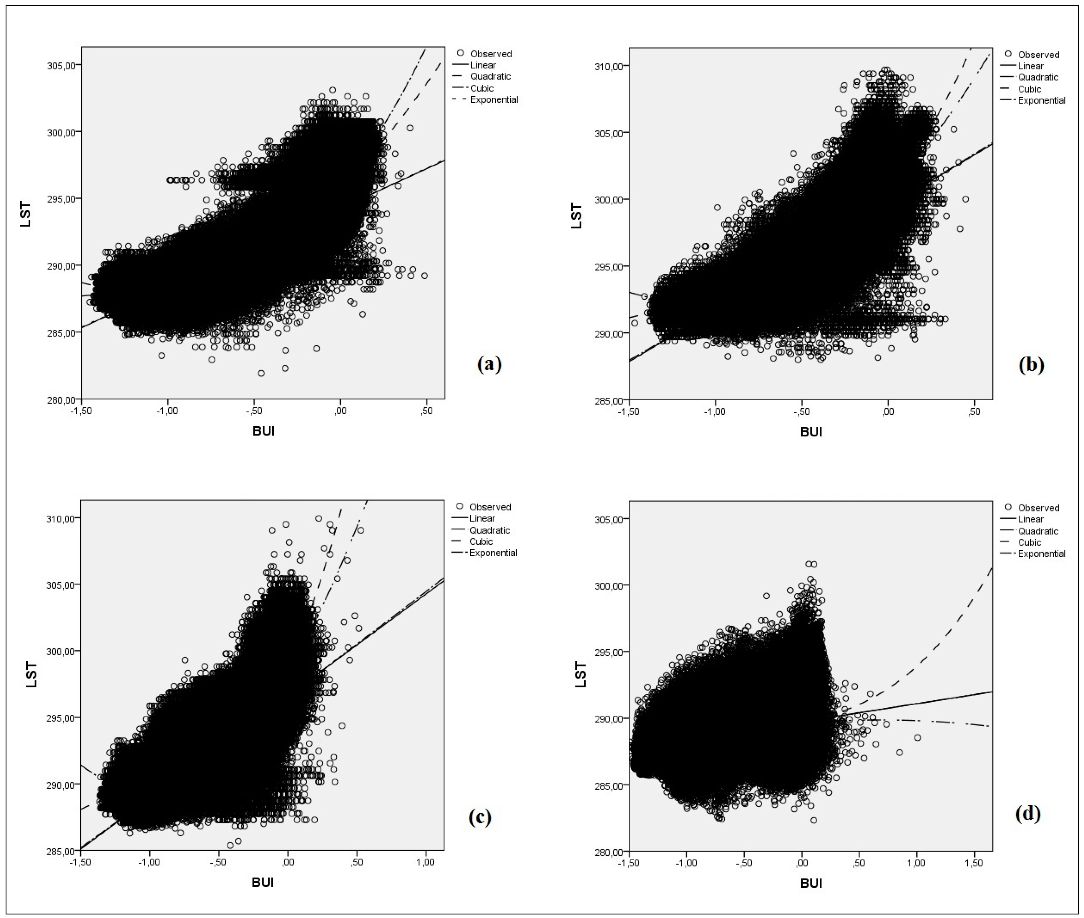
4.2. Statistical Analysis Between LST and Urbanization in Winter
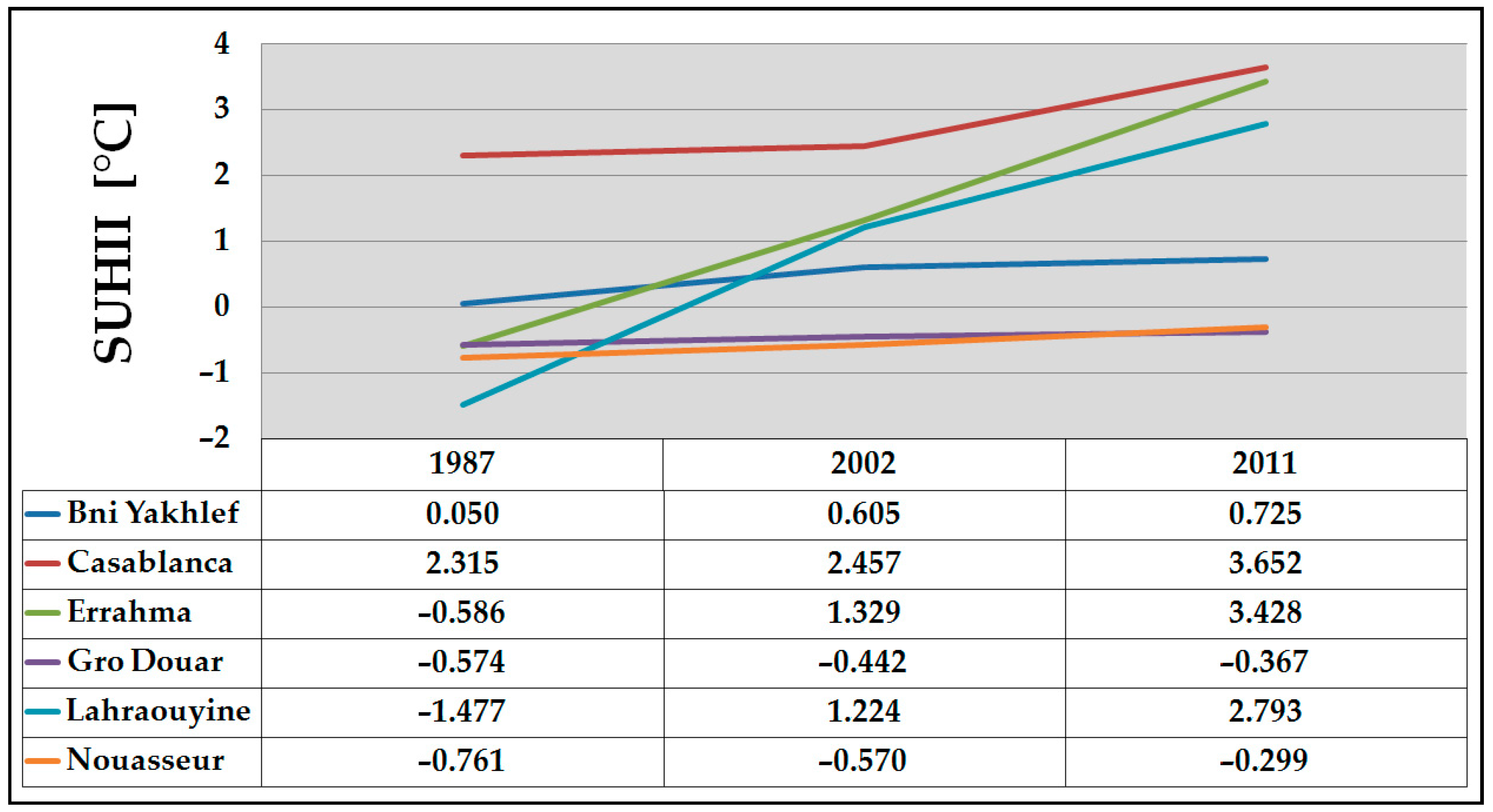
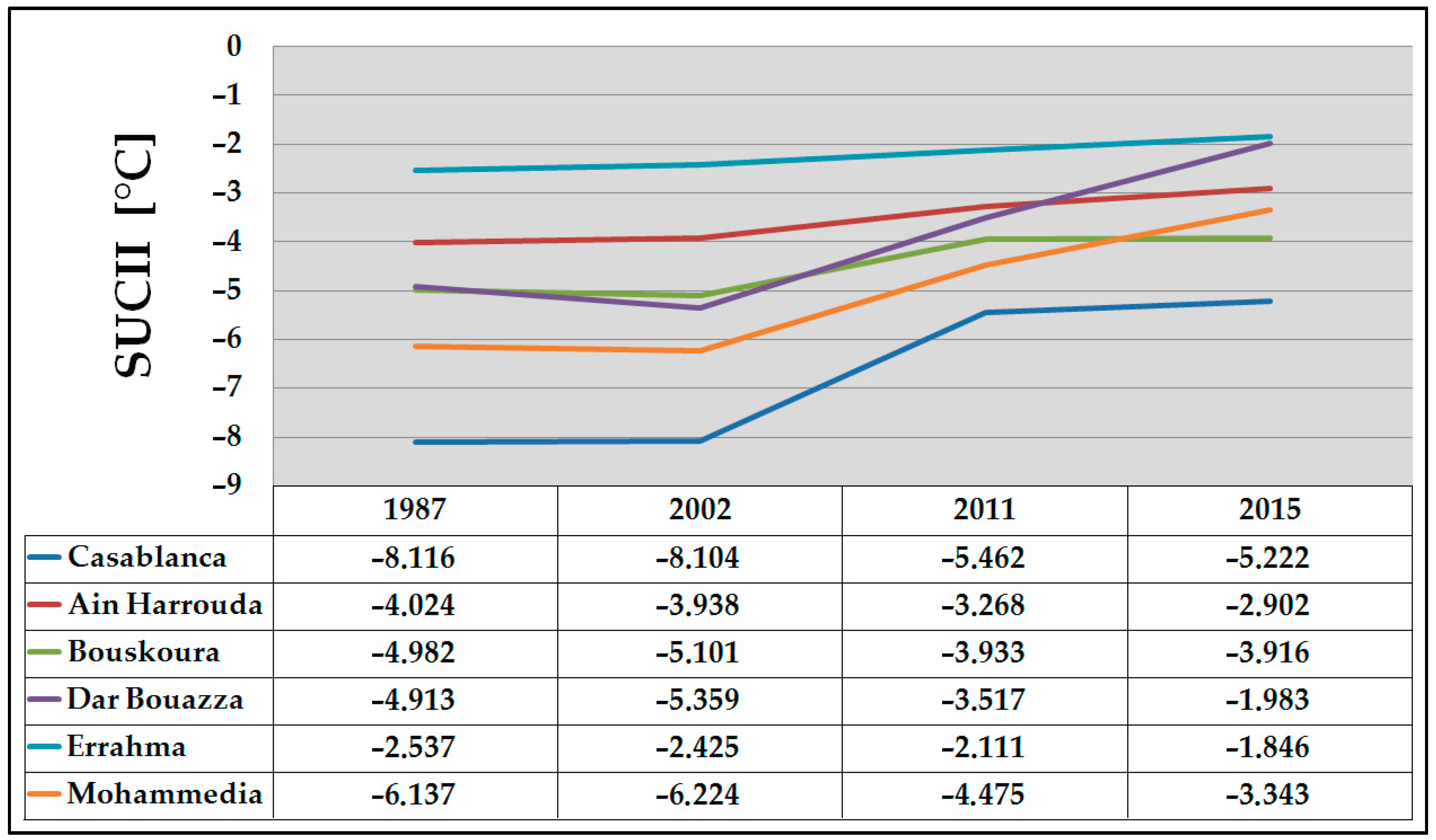
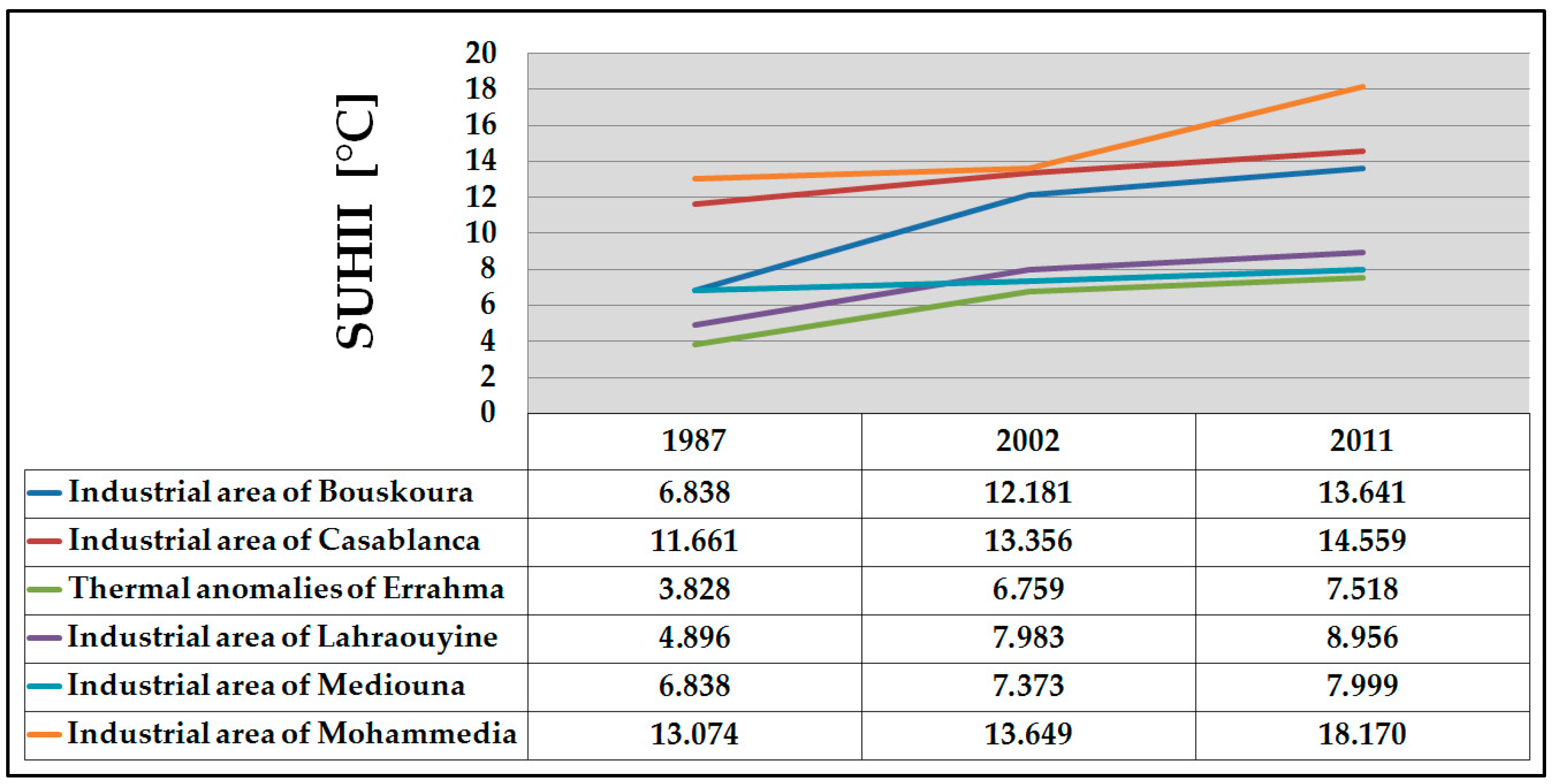
4.3. EvolutionAnalysis of SUHII in Winter
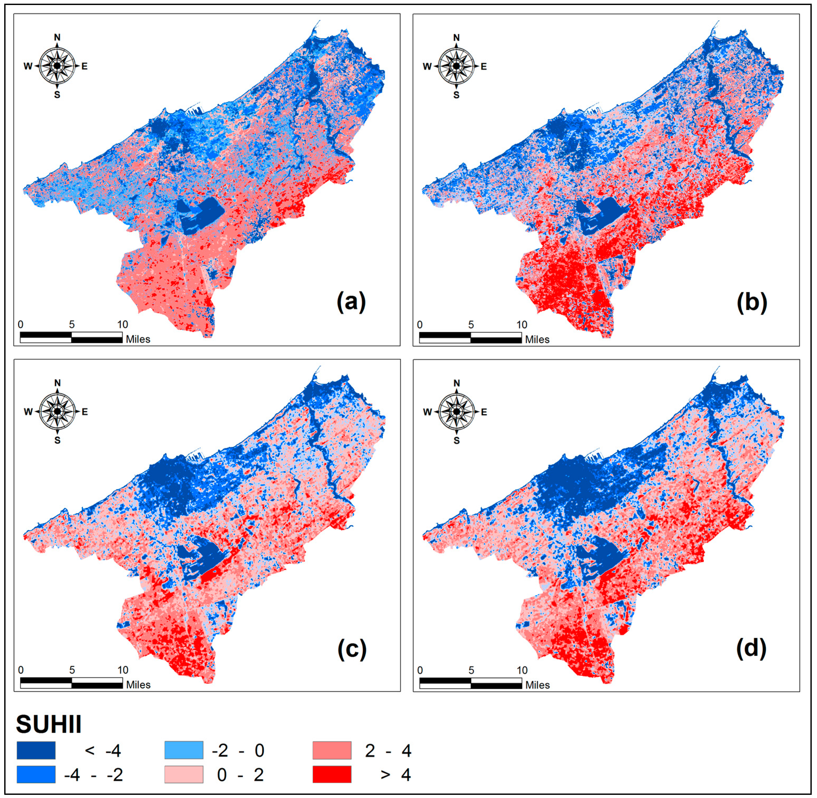
4.4. Spatio-Temporal Evolution of SUHII in Summer
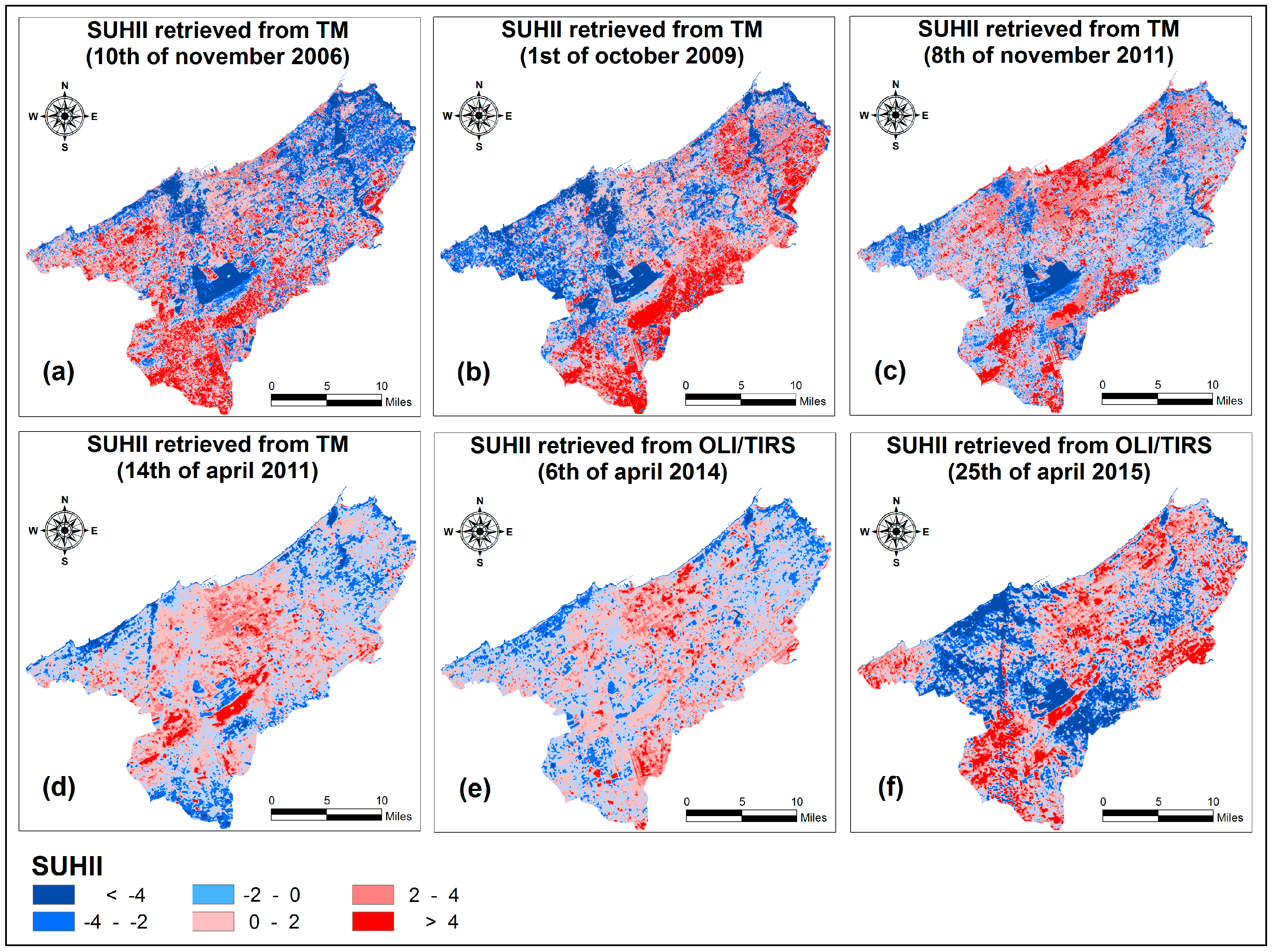
4.5. SUHII Pattern in Autumn and Spring Period
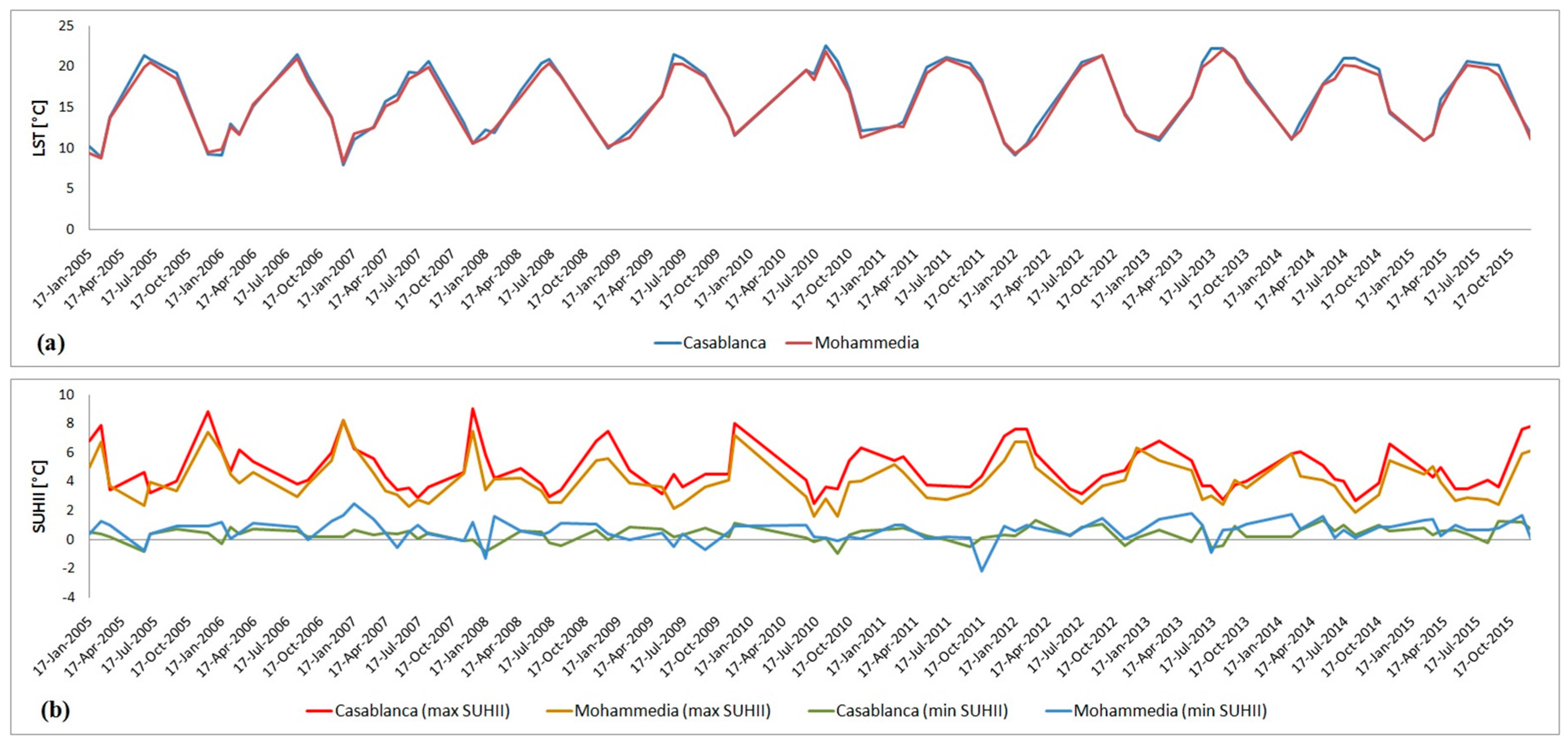
4.6. Variation of Nighttime SUHII
5. Discussions
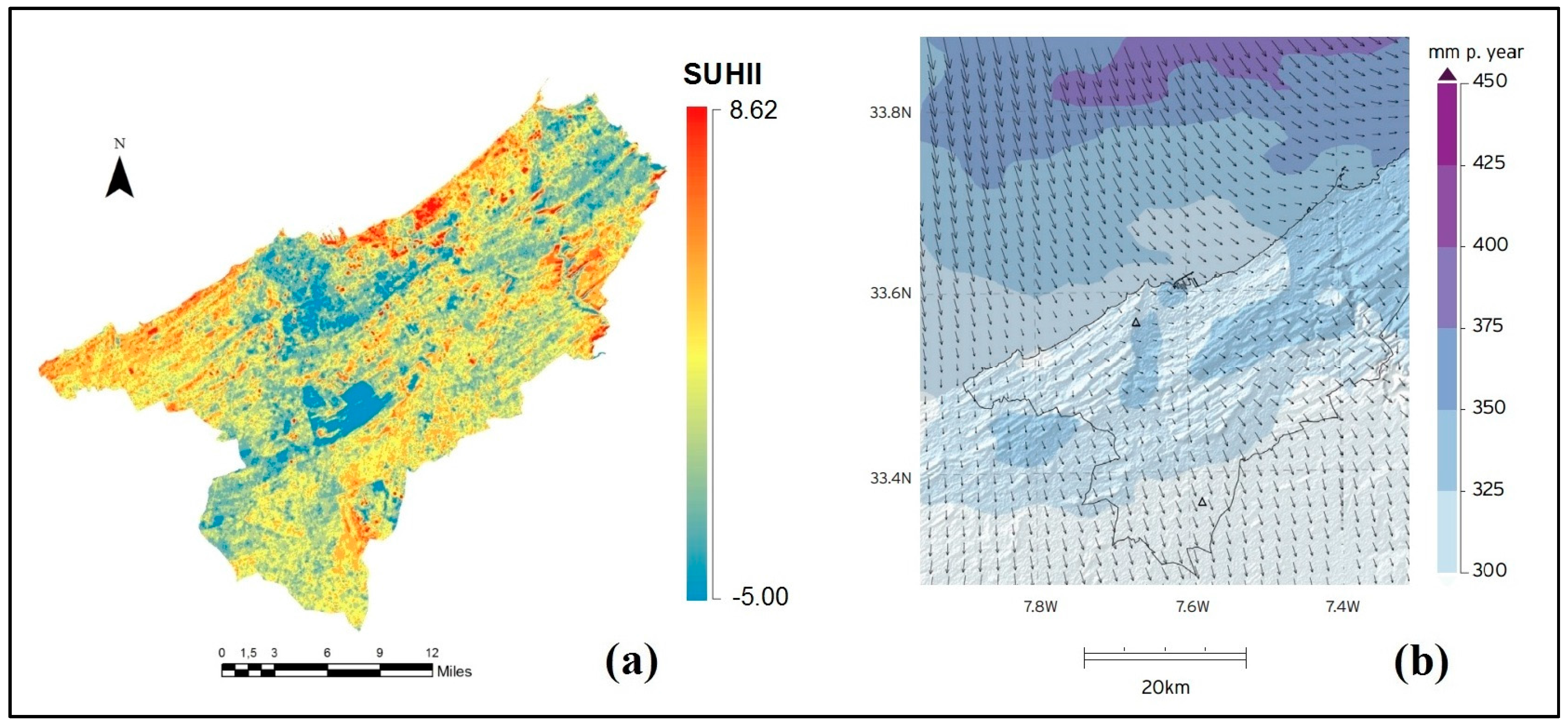
5.1. Climate Conditions Effect
5.2. Comparative Studies
6. Conclusions
Acknowledgments
Author Contributions
Conflicts of Interest
References
- United Nations Population Division—Department of Economic and Social Affairs. Available online: http://www.un.org/en/development/desa/population (accessed on 5 January 2016).
- Collier, C.G. The impact of urban areas on weather. Q. J. R. Meteorol. Soc. 2006, 132, 1–25. [Google Scholar] [CrossRef]
- Taha, H. Urban climates and heat islands: Albedo, evapotranspiration, and anthropogenic heat. Energy Build. 1997, 25, 99–103. [Google Scholar] [CrossRef]
- Boukhabl, M.; Alkam, D. Impact of vegetation on thermal conditions outside, thermal modeling of urban microclimate, case study: The Street of the Republic, Biskra. Energy Procedia 2012, 18, 73–84. [Google Scholar] [CrossRef]
- Goodin, D.G.; Harrington, J.A.; Rundquist, B.C. Land cover change and associated trends in surface reflectivity and vegetation index in Southwest Kansas: 1972–1992. Geocarto Int. 2002, 17, 45–52. [Google Scholar] [CrossRef]
- Cui, L.; Shi, J. Urbanization and its environmental effects in Shanghai, China. Urban Clim. 2012, 2, 1–15. [Google Scholar] [CrossRef]
- Zhang, Z.; Ji, M.; Shu, J.; Deng, Z.; Wu, Y. Surface urban heat island in Shanghai, China: Examining the relationship between land surface temperature and impervious surface fractions derived from Landsat ETM+ imagery. Int. Arch. Photogramm. Remote Sens. Spat. Inf. Sci. 2008, 37, 601–606. [Google Scholar]
- Tran, H.; Uchihama, D.; Ochi, S.; Yasuoka, Y. Assessment with satellite data of the urban heat island effects in Asian mega cities. Int. J. Appl. Earth Obs. Geoinf. 2006, 8, 34–48. [Google Scholar] [CrossRef]
- Streutker, D.R. A remote sensing study of the urban heat island of Houston, Texas. Int. J. Remote Sens. 2002, 23, 2595–2608. [Google Scholar] [CrossRef]
- Rhinane, H.; Hilali, A.; Bahi, H.; Berrada, A. Contribution of Landsat TM Data for the detection of urban heat islands areas case of Casablanca. J. Geogr. Inf. Syst. 2012, 4, 20–26. [Google Scholar]
- Sakhy, A.; Madelin, M.; Beltrando, G. Les échelles d’étude de l’îlot de chaleur urbain et ses relations avec la végétation et la géométriede la ville (exemple de Paris). In Proceedings of the Dixièmes Rencontres de Théo Quant, Paris, France, 23–25 February 2011.
- Tan, J.; Zheng, Y.; Tang, X.; Guo, C.; Li, L.; Song, G.; Zhen, X.; Yuan, D.; Kalkstein, A.J.; Li, F.; et al. The urban heat island and its impact on heat waves and human health in Shanghai. Int. J. Biometeorol. 2010, 54, 75–84. [Google Scholar] [CrossRef] [PubMed]
- Gong, P.; Liang, S.; Carlton, E.J.; Jiang, Q.; Wu, J.; Wang, L.; Remais, J.V. Urbanisation and health in China. Lancet 2012, 379, 843–852. [Google Scholar] [CrossRef]
- Muthers, S.; Matzarakis, A.; Koch, E. Summer climate and mortality in Vienna—A human-biometeorological approach of heat-related mortality during the heat waves in 2003. Wien. Klin. Wochenschr. 2010, 122, 525–531. [Google Scholar] [CrossRef] [PubMed]
- O’Loughlin, J.; Witmer, F.D.W.; Linke, A.M.; Laing, A.; Gettelman, A.; Dudhia, J. Climate variability and conflict risk in East Africa, 1990–2009. Proc. Natl. Acad. Sci. USA 2012, 109, 18344–18349. [Google Scholar] [CrossRef] [PubMed]
- Patz, J.A.; Campbell-Lendrum, D.; Holloway, T.; Foley, J.A. Impact of regional climate change on human health. Nature 2005, 438, 310–317. [Google Scholar] [CrossRef] [PubMed]
- Oke, T.R. The heat island of the urban boundary layer: Characteristics, causes and effects. In Wind Climate in Cities; Cermak, J.E., Davenport, A.G., Plate, E.J., Viegas, D.X., Eds.; Springer: Dordrecht, The Netherlands, 1995; pp. 81–107. [Google Scholar]
- Saaroni, H.; Ben-Dor, E.; Bitan, A.; Potchter, O. Spatial distribution and microscale characteristics of the urban heat island in Tel-Aviv, Israel. Landsc. Urban Plan. 2000, 48, 1–18. [Google Scholar] [CrossRef]
- Schwarz, N.; Lautenbach, S.; Seppelt, R. Exploring indicators for quantifying surface urban heat islands of European cities with MODIS land surface temperatures. Remote Sens. Environ. 2011, 115, 3175–3186. [Google Scholar] [CrossRef]
- Voogt, J.; Oke, T. Thermal remote sensing of urban climates. Remote Sens. Environ. 2003, 86, 370–384. [Google Scholar] [CrossRef]
- Bektaş Balçik, F. Determining the impact of urban components on land surface temperature of Istanbul by using remote sensing indices. Environ. Monit. Assess. 2014, 186, 859–872. [Google Scholar] [CrossRef] [PubMed]
- Weng, Q. Thermal infrared remote sensing for urban climate and environmental studies: Methods, applications, and trends. ISPRS J. Photogramm. Remote Sens. 2009, 64, 335–344. [Google Scholar] [CrossRef]
- Dihkan, M.; Karsli, F.; Guneroglu, A.; Guneroglu, N. Evaluation of surface urban heat island (SUHI) effect on coastal zone: The case of Istanbul Megacity. Ocean Coast. Manag. 2015, 118, 309–316. [Google Scholar] [CrossRef]
- Li, Y.; Zhang, H.; Kainz, W. Monitoring patterns of urban heat islands of the fast-growing Shanghai metropolis, China: Using time-series of Landsat TM/ETM+ data. Int. J. Appl. Earth Obs. Geoinf. 2012, 19, 127–138. [Google Scholar] [CrossRef]
- Wang, K.; Wang, J.; Wang, P.; Sparrow, M.; Yang, J.; Chen, H. Influences of urbanization on surface characteristics as derived from the moderate-resolution imaging spectroradiometer: A case study for the Beijing metropolitan area. J. Geophys. Res. 2007. [Google Scholar] [CrossRef]
- Frey, C.M.; Kuenzer, C.; Dech, S. Quantitative comparison of the operational NOAA-AVHRR LST product of DLR and the MODIS LST product V005. Int. J. Remote Sens. 2012, 33, 7165–7183. [Google Scholar] [CrossRef]
- Mao, K.; Qin, Z.; Shi, J.; Gong, P. A practical split-window algorithm for retrieving land-surface temperature from MODIS data. Int. J. Remote Sens. 2005, 26, 3181–3204. [Google Scholar] [CrossRef]
- Kato, S.; Yamaguchi, Y. Analysis of urban heat-island effect using ASTER and ETM+ Data: Separation of anthropogenic heat discharge and natural heat radiation from sensible heat flux. Remote Sens. Environ. 2005, 99, 44–54. [Google Scholar] [CrossRef]
- Lu, D.; Weng, Q. Spectral mixture analysis of ASTER images for examining the relationship between urban thermal features and biophysical descriptors in Indianapolis, Indiana, USA. Remote Sens. Environ. 2006, 104, 157–167. [Google Scholar] [CrossRef]
- Liu, H.; Weng, Q. Seasonal variations in the relationship between landscape pattern and land surface temperature in Indianapolis, USA. Environ. Monit. Assess. 2008, 144, 199–219. [Google Scholar] [CrossRef] [PubMed]
- Weng, Q.; Lu, D.; Schubring, J. Estimation of land surface temperature—Vegetation abundance relationship for urban heat island studies. Remote Sens. Environ. 2004, 89, 467–483. [Google Scholar] [CrossRef]
- Yue, W.; Xu, J.; Tan, W.; Xu, L. The relationship between land surface temperature and NDVI with remote sensing: Application to Shanghai Landsat 7 ETM+ data. Int. J. Remote Sens. 2007, 28, 3205–3226. [Google Scholar] [CrossRef]
- Xiao, R.; Weng, Q.; Ouyang, Z.; Li, W.; Schienke, E.W.; Zhang, Z. Land surface temperature variation and major factors in Beijing, China. Photogramm. Eng. Remote Sens. 2008, 74, 451–461. [Google Scholar] [CrossRef]
- Elvidge, C.D.; Baugh, K.E.; Kihn, E.A.; Kroehl, H.W.; Davis, E.R.; Davis, C.W. Relation between satellite observed visible-near infrared emissions, population, economic activity and electric power consumption. Int. J. Remote Sens. 1997, 18, 1373–1379. [Google Scholar] [CrossRef]
- Ghobadi, Y.; Pradhan, B.; Shafri, H.Z.M.; Kabiri, K. Assessment of spatial relationship between land surface temperature and land use/cover retrieval from multi-temporal remote sensing data in South Karkheh Sub-basin, Iran. Arab. J. Geosci. 2015, 8, 525–537. [Google Scholar] [CrossRef]
- Tan, K.C.; Lim, H.S.; Mat Jafri, M.Z.; Abdullah, K. A comparison of radiometric correction techniques in the evaluation of the relationship between LST and NDVI in Landsat imagery. Environ. Monit. Assess. 2012, 184, 3813–3829. [Google Scholar] [CrossRef] [PubMed]
- Gallo, K.P.; Tarpley, J.D.; McNab, A.L.; Karl, T.R. Assessment of urban heat islands: A satellite perspective. Atmos. Res. 1995, 37, 37–43. [Google Scholar] [CrossRef]
- Nie, Q.; Xu, J. Understanding the effects of the impervious surfaces pattern on land surface temperature in an urban area. Front. Earth Sci. 2015, 9, 276–285. [Google Scholar] [CrossRef]
- Imhoff, M.L.; Zhang, P.; Wolfe, R.E.; Bounoua, L. Remote sensing of the urban heat island effect across biomes in the continental USA. Remote Sens. Environ. 2010, 114, 504–513. [Google Scholar] [CrossRef]
- Stathopoulou, M.; Cartalis, C. Daytime urban heat islands from Landsat ETM+ and Corine land cover data: An application to major cities in Greece. Sol. Energy 2007, 81, 358–368. [Google Scholar] [CrossRef]
- Dousset, B.; Gourmelon, F.; Laaidi, K.; Zeghnoun, A.; Giraudet, E.; Bretin, P.; Mauri, E.; Vandentorren, S. Satellite monitoring of summer heat waves in the Paris metropolitan area. Int. J. Climatol. 2011, 31, 313–323. [Google Scholar] [CrossRef]
- Hu, Y.; Jia, G. Influence of land use change on urban heat island derived from multi-sensor data. Int. J. Climatol. 2009. [Google Scholar] [CrossRef]
- Clinton, N.; Gong, P. MODIS detected surface urban heat islands and sinks: Global locations and controls. Remote Sens. Environ. 2013, 134, 294–304. [Google Scholar] [CrossRef]
- Ichinose, T.; Shimodozono, K.; Hanaki, K. Impact of anthropogenic heat on urban climate in Tokyo. Atmos. Environ. 1999, 33, 3897–3909. [Google Scholar] [CrossRef]
- Zhou, D.; Zhao, S.; Liu, S.; Zhang, L.; Zhu, C. Surface urban heat island in China’s 32 major cities: Spatial patterns and drivers. Remote Sens. Environ. 2014, 152, 51–61. [Google Scholar] [CrossRef]
- Peng, S.; Piao, S.; Ciais, P.; Friedlingstein, P.; Ottle, C.; Bréon, F.-M.; Nan, H.; Zhou, L.; Myneni, R.B. Surface urban heat island across 419 global big cities. Environ. Sci. Technol. 2012, 46, 696–703. [Google Scholar] [CrossRef] [PubMed]
- Feng, H.; Liu, Y. Combined effects of precipitation and air temperature on soil moisture in different land covers in a humid basin. J. Hydrol. 2015, 531, 1129–1140. [Google Scholar] [CrossRef]
- Sakaida, K.; Egoshi, A.; Kuramochi, M. Effects of sea breezes on mitigating urban heat island phenomenon: Vertical observation results in the urban center of Sendai. J. Geogr. 2011, 120, 382–391. [Google Scholar] [CrossRef]
- Moulali, T. L’émigration Internationale et le Problème du Retour à Casablanca; Université des Sciences et Technologies: Lille, France, 1992. [Google Scholar]
- Giseke, U.; Gerster-Bentaya, M.; Helten, F.; Kraume, M.; Scherer, D.; Spars, G.; Amraoui, F.; Adidi, A.; Berdouz, S.; Chlaida, M.; et al. Urban Agriculture for Growing City Regions: Connecting Urban-Rural Spheres in Casablanca; Routledge: Abingdon, VI, USA, 2015. [Google Scholar]
- Roy, D.P.; Wulder, M.A.; Loveland, T.R.; Woodcock, C.E.; Allen, R.G.; Anderson, M.C.; Helder, D.; Irons, J.R.; Johnson, D.M.; Kennedy, R.; et al. Landsat-8: Science and product vision for terrestrial global change research. Remote Sens. Environ. 2014, 145, 154–172. [Google Scholar] [CrossRef]
- Irons, J.R.; Dwyer, J.L.; Barsi, J.A. The next Landsat satellite: The Landsat data continuity mission. Remote Sens. Environ. 2012, 122, 11–21. [Google Scholar] [CrossRef]
- Chander, G.; Markham, B.L.; Barsi, J.A. Revised Landsat-5 Thematic Mapper Radiometric calibration. IEEE Geosci. Remote Sens. Lett. 2007, 4, 490–494. [Google Scholar] [CrossRef]
- Markham, B.; Barsi, J.; Kvaran, G.; Ong, L.; Kaita, E.; Biggar, S.; Czapla-Myers, J.; Mishra, N.; Helder, D. Landsat-8 operational land imager radiometric calibration and stability. Remote Sens. 2014, 6, 12275–12308. [Google Scholar] [CrossRef]
- Czapla-Myers, J.; McCorkel, J.; Anderson, N.; Thome, K.; Biggar, S.; Helder, D.; Aaron, D.; Leigh, L.; Mishra, N. The ground-based absolute radiometric calibration of Landsat 8 OLI. Remote Sens. 2015, 7, 600–626. [Google Scholar] [CrossRef]
- Chander, G.; Markham, B.L.; Helder, D.L. Summary of current radiometric calibration coefficients for Landsat MSS, TM, ETM+, and EO-1 ALI sensors. Remote Sens. Environ. 2009, 113, 893–903. [Google Scholar] [CrossRef]
- Chen, D.; Brutsaert, W. Satellite-Sensed Distribution and Spatial Patterns of Vegetation Parameters over a Tallgrass Prairie. J. Atmos. Sci. 1998, 55, 1225–1238. [Google Scholar] [CrossRef]
- Yuvaraj, E.; Dharanirajan, K.; Saravanan, N.K. Evaluation of Vegetation density of the Mangrove forest in South Andaman Island using Remote Sensing and GIS techniques. Int. Res. J. Environ. Sci. 2014, 3, 19–25. [Google Scholar]
- Verrelst, J.; Romijn, E.; Kooistra, L. Mapping vegetation density in a heterogeneous river floodplain ecosystem using pointable CHRIS/PROBA data. Remote Sens. 2012, 4, 2866–2889. [Google Scholar] [CrossRef]
- Bunn, A.G.; Goetz, S.J. Trends in Satellite-observed circumpolar photosynthetic activity from 1982 to 2003: The influence of seasonality, cover type, and vegetation density. Earth Interact. 2006, 10, 1–19. [Google Scholar] [CrossRef]
- Tucker, C.J. Red and photographic infrared linear combinations for monitoring vegetation. Remote Sens. Environ. 1979, 8, 127–150. [Google Scholar] [CrossRef]
- Bannari, A.; Teillet, P.M.; Landry, R. Comparaison des réflectances de surfaces naturelles dans les bandes spectrales homologues des capteurs TM de Landsat-5 ET ETM+ de Landsat-7. Télédétection 2004, 4, 263–275. [Google Scholar]
- Roy, D.P.; Kovalskyy, V.; Zhang, H.K.; Vermote, E.F.; Yan, L.; Kumar, S.S.; Egorov, A. Characterization of Landsat-7 to Landsat-8 reflective wavelength and normalized difference vegetation index continuity. Remote Sens. Environ. 2016. [Google Scholar] [CrossRef]
- Mishra, N.; Haque, M.; Leigh, L.; Aaron, D.; Helder, D.; Markham, B. Radiometric cross calibration of Landsat 8 Operational Land Imager (OLI) and Landsat 7 Enhanced Thematic Mapper Plus (ETM+). Remote Sens. 2014, 6, 12619–12638. [Google Scholar] [CrossRef]
- Teillet, P.; Barker, J.; Markham, B.; Irish, R.; Fedosejevs, G.; Storey, J. Radiometric cross-calibration of the Landsat-7 ETM+ and Landsat-5 TM sensors based on tandem data sets. Remote Sens. Environ. 2001, 78, 39–54. [Google Scholar] [CrossRef]
- Figoski, J.W.; Zaun, N.; Mooney, T. Performance results for the Landsat OLI spectral filters. Proc. SPIE 2009. [Google Scholar] [CrossRef]
- Li, P.; Jiang, L.; Feng, Z. Cross-comparison of vegetation indices derived from Landsat-7 Enhanced Thematic Mapper Plus (ETM+) and Landsat-8 Operational Land Imager (OLI) sensors. Remote Sens. 2013, 6, 310–329. [Google Scholar] [CrossRef]
- Barsi, J.; Lee, K.; Kvaran, G.; Markham, B.; Pedelty, J. The spectral response of the Landsat-8 operational land imager. Remote Sens. 2014, 6, 10232–10251. [Google Scholar] [CrossRef]
- Valor, E. Mapping land surface emissivity from NDVI: Application to European, African, and South American areas. Remote Sens. Environ. 1996, 57, 167–184. [Google Scholar] [CrossRef]
- Li, X.; Li, W.; Middel, A.; Harlan, S.L.; Brazel, A.J.; Turner, B.L. Remote sensing of the surface urban heat island and land architecture in Phoenix, Arizona: Combined effects of land composition and configuration and cadastral demographic—Economic factors. Remote Sens. Environ. 2016, 174, 233–243. [Google Scholar] [CrossRef]
- Sobrino, J.A.; Jimenez-Muoz, J.C.; Soria, G.; Romaguera, M.; Guanter, L.; Moreno, J.; Plaza, A.; Martinez, P. Land Surface Emissivity Retrieval From Different VNIR and TIR Sensors. IEEE Trans. Geosci. Remote Sens. 2008, 46, 316–327. [Google Scholar] [CrossRef]
- Yu, X.; Guo, X.; Wu, Z. Land surface temperature retrieval from Landsat 8 TIRS—Comparison between radiative transfer equation-based method, split window algorithm and single channel method. Remote Sens. 2014, 6, 9829–9852. [Google Scholar] [CrossRef]
- Sobrino, J.A.; Raissouni, N. Toward remote sensing methods for land cover dynamic monitoring: Application to Morocco. Int. J. Remote Sens. 2000, 21, 353–366. [Google Scholar] [CrossRef]
- Carlson, T.N.; Ripley, D.A. On the relation between NDVI, fractional vegetation cover, and leaf area index. Remote Sens. Environ. 1997, 62, 241–252. [Google Scholar] [CrossRef]
- Allen, R.G.; Tasumi, M.; Morse, A.; Trezza, R.; Wright, J.L.; Bastiaanssen, W.; Kramber, W.; Lorite, I.; Robison, C.W. Satellite-Based energy balance for Mapping Evapotranspiration with Internalized Calibration (METRIC)—Applications. J. Irrig. Drain. Eng. 2007, 133, 395–406. [Google Scholar] [CrossRef]
- Anderson, M.C.; Norman, J.M.; Mecikalski, J.R.; Otkin, J.A.; Kustas, W.P. A climatological study of evapotranspiration and moisture stress across the continental United States based on thermal remote sensing: 1. Model formulation. J. Geophys. Res. 2007. [Google Scholar] [CrossRef]
- Bechtel, B.; Zakšek, K.; Hoshyaripour, G. Downscaling land surface temperature in an urban area: A Case study for Hamburg, Germany. Remote Sens. 2012, 4, 3184–3200. [Google Scholar] [CrossRef]
- Zakšek, K.; Oštir, K. Downscaling land surface temperature for urban heat island diurnal cycle analysis. Remote Sens. Environ. 2012, 117, 114–124. [Google Scholar] [CrossRef]
- Ayanlade, A.; Jegede, O.O. Evaluation of the intensity of the daytime surface urban heat island: How can remote sensing help? Int. J. Image Data Fusion 2015, 6, 348–365. [Google Scholar] [CrossRef]
- Qin, Z.; Karnieli, A.; Berliner, P. A mono-window algorithm for retrieving land surface temperature from Landsat TM data and its application to the Israel-Egypt border region. Int. J. Remote Sens. 2001, 22, 3719–3746. [Google Scholar] [CrossRef]
- Jiménez-Muñoz, J.C. A generalized single-channel method for retrieving land surface temperature from remote sensing data. J. Geophys. Res. 2003. [Google Scholar] [CrossRef]
- Sobrino, J.A.; Caselles, V.; Coll, C. Theoretical split-window algorithms for determining the actual surface temperature. IL Nuovo Cimento 1993, 16, 219–236. [Google Scholar] [CrossRef]
- Becker, F.; Li, Z.L. Towards a local split window method over land surfaces. Int. J. Remote Sens. 1990, 11, 369–393. [Google Scholar] [CrossRef]
- Sobrino, J.A.; Sòria, G.; Prata, A.J. Surface temperature retrieval from Along Track Scanning Radiometer 2 data: Algorithms and validation. J. Geophys. Res. 2004. [Google Scholar] [CrossRef]
- Chedin, A.; Scott, N.A.; Berroir, A. A Single-Channel, double-viewing angle method for sea surface temperature determination from coincident METEOSAT and TIROS-N radiometric measurements. J. Appl. Meteorol. 1982, 21, 613–618. [Google Scholar] [CrossRef]
- Prata, A.J. Land surface temperatures derived from the advanced very high resolution radiometer and the along-track scanning radiometer: 1. Theory. J. Geophys. Res. 1993. [Google Scholar] [CrossRef]
- Zhaoliang, L.; Stoll, M.P.; Renhua, Z.; Li, J.; Zhongbo, S. On the separate retrieval of soil and vegetation temperatures from ATSR data. Sci. Chin. Ser. Earth Sci. 2001, 44, 97–111. [Google Scholar] [CrossRef]
- Artis, D.A.; Carnahan, W.H. Survey of emissivity variability in thermography of urban areas. Remote Sens. Environ. 1982, 12, 313–329. [Google Scholar] [CrossRef]
- Sobrino, J.; Coll, C.; Caselles, V. Atmospheric correction for land surface temperature using NOAA-11 AVHRR channels 4 and 5. Remote Sens. Environ. 1991, 38, 19–34. [Google Scholar] [CrossRef]
- Du, C.; Ren, H.; Qin, Q.; Meng, J.; Zhao, S. A Practical split-window algorithm for estimating land surface temperature from Landsat 8 data. Remote Sens. 2015, 7, 647–665. [Google Scholar] [CrossRef]
- Zha, Y.; Gao, J.; Ni, S. Use of normalized difference built-up index in automatically mapping urban areas from TM imagery. Int. J. Remote Sens. 2003, 24, 583–594. [Google Scholar] [CrossRef]
- Xu, H. A new index for delineating built-up land features in satellite imagery. Int. J. Remote Sens. 2008, 29, 4269–4276. [Google Scholar] [CrossRef]
- Holsten, A.; Vetter, T.; Vohland, K.; Krysanova, V. Impact of climate change on soil moisture dynamics in Brandenburg with a focus on nature conservation areas. Ecol. Model. 2009, 220, 2076–2087. [Google Scholar] [CrossRef]
- Wang, G.; Li, Y.; Hu, H.; Wang, Y. Synergistic effect of vegetation and air temperature changes on soil water content in alpine frost meadow soil in the permafrost region of Qinghai-Tibet. Hydrol. Process. 2008, 22, 3310–3320. [Google Scholar] [CrossRef]
- Freedman, M.; Jaggi, B. Global warming, commitment to the Kyoto protocol, and accounting disclosures by the largest global public firms from polluting industries. Int. J. Account. 2005, 40, 215–232. [Google Scholar] [CrossRef]
- Daniel, B.; Stanisstreet, M.; Boyes, E. How can we best reduce global warming? School students’ ideas and misconceptions. Int. J. Environ. Stud. 2004, 61, 211–222. [Google Scholar] [CrossRef]
- Lashof, D.A.; Ahuja, D.R. Relative contributions of greenhouse gas emissions to global warming. Nature 1990, 344, 529–531. [Google Scholar] [CrossRef]
- Shine, K.P.; Fuglestvedt, J.S.; Hailemariam, K.; Stuber, N. Alternatives to the global warming potential for comparing climate impacts of emissions of greenhouse gases. Clim. Chang. 2005, 68, 281–302. [Google Scholar] [CrossRef]
- Cartalis, C. Climatic Change in the built environment in temperate climates with emphasis on the Mediterranean Area. In Energy Performance of Buildings; Boemi, S.N., Irulegi, O., Santamouris, M., Eds.; Springer International Publishing: Cham, Switzerland, 2016; pp. 19–36. [Google Scholar]
- Zhang, J.; Li, Y.; Wang, Y. Monitoring the urban heat island and the spatial expansion: Using thermal remote sensing image of ETM+ band6. Proc. SPIE 2007. [Google Scholar] [CrossRef]
- Abraha, M.G.; Savage, M.J. Potential impacts of climate change on the grain yield of maize for the midlands of KwaZulu-Natal, South Africa. Agric. Ecosyst. Environ. 2006, 115, 150–160. [Google Scholar] [CrossRef]
- Kang, Y.; Khan, S.; Ma, X. Climate change impacts on crop yield, crop water productivity and food security—A review. Prog. Nat. Sci. 2009, 19, 1665–1674. [Google Scholar] [CrossRef]
- Patz, J.A.; Gibbs, H.K.; Foley, J.A.; Rogers, J.V.; Smith, K.R. Climate change and global health: Quantifying a growing ethical crisis. EcoHealth 2007, 4, 397–405. [Google Scholar] [CrossRef]
- Magadza, C.H. Climate Change Impacts and Human Settlements in Africa: Prospects for adaptation. Environ. Monit. Assess. 2000, 61, 193–205. [Google Scholar] [CrossRef]
- Santamouris, M. Analyzing the heat island magnitude and characteristics in one hundred Asian and Australian cities and regions. Sci. Total Environ. 2015, 512–513, 582–598. [Google Scholar] [CrossRef] [PubMed]
- Sashiyama, S.; Yamamoto, K. Method for evaluating the influence of obstruction of Sea Breeze by clusters of high-rise buildings on the urban heat island effect. J. Environ. Prot. 2014, 5, 983–996. [Google Scholar] [CrossRef]
- Ohashi, Y.; Kida, H. Local Circulations Developed in the vicinity of both coastal and inland urban areas: A numerical study with a mesoscale atmospheric model. J. Appl. Meteorol. 2002, 41, 30–45. [Google Scholar] [CrossRef]
- Chow, W.T.L.; Roth, M. Temporal dynamics of the urban heat island of Singapore. Int. J. Climatol. 2006, 26, 2243–2260. [Google Scholar] [CrossRef]
- Quan, J.; Zhan, W.; Chen, Y.; Wang, M.; Wang, J. Time series decomposition of remotely sensed land surface temperature and investigation of trends and seasonal variations in surface urban heat islands: Thermal image series decomposition. J. Geophys. Res. Atmos. 2016, 121, 2638–2657. [Google Scholar] [CrossRef]
- Yuan, F.; Bauer, M.E. Comparison of impervious surface area and normalized difference vegetation index as indicators of surface urban heat island effects in Landsat imagery. Remote Sens. Environ. 2007, 106, 375–386. [Google Scholar] [CrossRef]
- Oke, T.R. The energetic basis of the urban heat island. Q. J. R. Meteorol. Soc. 1982, 108, 1–24. [Google Scholar] [CrossRef]
- Stewart, I.D.; Oke, T.R. Local Climate zones for urban temperature studies. Bull. Am. Meteorol. Soc. 2012, 93, 1879–1900. [Google Scholar] [CrossRef]
- Nichol, J.E. High-Resolution surface temperature patterns related to urban morphology in a tropical city: A Satellite-based study. J. Appl. Meteorol. 1996, 35, 135–146. [Google Scholar] [CrossRef]
- Hall, A. The role of surface albedo feedback in climate. J. Clim. 2004, 17, 1550–1568. [Google Scholar] [CrossRef]
- Santamouris, M.; Papanikolaou, N.; Livada, I.; Koronakis, I.; Georgakis, C.; Argiriou, A.; Assimakopoulos, D. On the impact of urban climate on the energy consumption of buildings. Sol. Energy 2001, 70, 201–216. [Google Scholar] [CrossRef]
- Lofgren, B.M.; Hunter, T.S.; Wilbarger, J. Effects of using air temperature as a proxy for potential evapotranspiration in climate change scenarios of Great Lakes basin hydrology. J. Gt. Lakes Res. 2011, 37, 744–752. [Google Scholar] [CrossRef]
- Lakshmi, V.; Zehrfuhs, D.; Jackson, T. Observations of land surface temperature and its relationship to soil moisture during SGP99. In Proceedings of the IEEE 2000 International Geoscience and Remote Sensing Symposium, Honolulu, HI, USA, 24–28 July 2000; pp. 1256–1258.
- Runnalls, K.E.; Oke, T.R. Dynamics and controls of the near surface heat island of Vancouver, British Columbia. Phys. Geogr. 2000, 21, 283–304. [Google Scholar]
- Zhao, L.; Lee, X.; Smith, R.B.; Oleson, K. Strong contributions of local background climate to urban heat islands. Nature 2014, 511, 216–219. [Google Scholar] [CrossRef] [PubMed]
- Cohen, P.; Potchter, O.; Matzarakis, A. Daily and seasonal climatic conditions of green urban open spaces in the Mediterranean climate and their impact on human comfort. Build. Environ. 2012, 51, 285–295. [Google Scholar] [CrossRef]
- Schwarz, N.; Schlink, U.; Franck, U.; Großmann, K. Relationship of land surface and air temperatures and its implications for quantifying urban heat island indicators—An application for the city of Leipzig (Germany). Ecol. Indic. 2012, 18, 693–704. [Google Scholar] [CrossRef]
- Jauregui, E.; Godinez, L.; Cruz, F. Aspects of heat-island development in Guadalajara, Mexico. Atmos. Environ. Part B Urban Atmos. 1992, 26, 391–396. [Google Scholar] [CrossRef]
- Sakaida, K.; Egoshi, A. Influences of Sea Breeze on Urban Heat Island in Sendai, Japan; Inspiro AB: Göteborg, Sweden, 2006; pp. 388–391. [Google Scholar]
- Tokairin, T.; Kondo, H.; Kikegawa, Y. Potential of Sea Breeze from The Tokyo Bay for Natural Ventilation in Buildings; Inspiro AB: Göteborg, Sweden, 2006; pp. 525–527. [Google Scholar]
- Zhou, D.; Zhang, L.; Hao, L.; Sun, G.; Liu, Y.; Zhu, C. Spatiotemporal trends of urban heat island effect along the urban development intensity gradient in China. Sci. Total Environ. 2016, 544, 617–626. [Google Scholar] [CrossRef] [PubMed]
- Wilby, R.L. Past and projected trends in London’s urban heat island. Weather 2003, 58, 251–260. [Google Scholar] [CrossRef]
- Kłysik, K.; Fortuniak, K. Temporal and spatial characteristics of the urban heat island of Łódź, Poland. Atmos. Environ. 1999, 33, 3885–3895. [Google Scholar] [CrossRef]
- Benas, N.; Chrysoulakis, N.; Poursanidis, D. The surface urban heat island in large Mediterranean cities during the last decade: Annual characteristics and trends based on EO data. In Proceedings of the Mediterranean City 2014: Adaptation Strategies to Global Environmental Change in the Mediterranean City and the Role of Global Earth Observations, Athens, Greece, 10–11 June 2014.
- Mihalakakou, G.; Santamouris, M.; Papanikolaou, N.; Cartalis, C.; Tsangrassoulis, A. Simulation of the urban heat island phenomenon in Mediterranean climates. Pure Appl. Geophys. 2004, 161, 429–451. [Google Scholar] [CrossRef]
- Giannaros, T.M.; Melas, D. Study of the urban heat island in a coastal Mediterranean City: The case study of Thessaloniki, Greece. Atmos. Res. 2012, 118, 103–120. [Google Scholar] [CrossRef]
- Poupkou, A.; Nastos, P.; Melas, D.; Zerefos, C. Climatology of discomfort index and air quality index in a large urban Mediterranean agglomeration. Water. Air. Soil Pollut. 2011, 222, 163–183. [Google Scholar] [CrossRef]


| Landsat Product | Acquisition Date | Path/Row | Spatial Resolution of TIR Band (m) | Id-Scene Information | Cycle |
|---|---|---|---|---|---|
| Landsat TM | 25 August 1984 | 202/37 | 120 | LT52020371984238XXX04 | Daytime |
| Landsat TM | 7 February 1987 | 202/37 | 120 | LT52020371987038XXX08 | Daytime |
| Landsat ETM+ | 8 February 2002 | 202/37 | 60 | LE72020372002039EDC00 | Daytime |
| Landsat TM | 30 August 2003 | 202/37 | 120 | LT52020372003242MTI01 | Daytime |
| Landsat TM | 10 November 2006 | 202/37 | 120 | LT52020372006314MPS00 | Daytime |
| Landsat TM | 1 October 2009 | 202/37 | 120 | LT52020372009274MPS00 | Daytime |
| Landsat TM | 8 January 2011 | 202/37 | 120 | LT52020372011008MPS00 | Daytime |
| Landsat TM | 14 April 2011 | 202/37 | 120 | LT52020372011104MPS00 | Daytime |
| Landsat TM | 8 November 2011 | 202/37 | 120 | LT52020372011312MPS01 | Daytime |
| Landsat OLI/TIRS | 24 July 2013 | 202/37 | 100 | LC82020372013205LGN00 | Daytime |
| Landsat OLI/TIRS | 6 April 2014 | 202/37 | 100 | LC82020372014096LGN00 | Daytime |
| Landsat OLI/TIRS | 12 August 2014 | 202/37 | 100 | LC82020372014224LGN00 | Daytime |
| Landsat OLI/TIRS | 3 January 2015 | 202/37 | 100 | LC82020372015003LGN00 | Daytime |
| Landsat OLI/TIRS | 25 April 2015 | 202/37 | 100 | LC82020372015115LGN00 | Daytime |
| Landsat OLI/TIRS | 17 June 2015 | 68/207 | 100 | LC80682072015168LGN00 | Nighttime |
| Landsat OLI/TIRS | 6 January 2016 | 202/37 | 100 | LC82020372016006LGN00 | Daytime |
| Landsat 5 TM Band 6 | Landsat 7 ETM+ Band 6 | Landsat 8 TIRS | ||
|---|---|---|---|---|
| Band 10 | Band 11 | |||
| K1 [K] | 607.76 | 666.09 | 774.89 | 480.89 |
| K2 [W/(m2 sr μm)] | 1260.56 | 1282.71 | 1321.08 | 1201.14 |
| Classes | Daytime SUHII Range (°C) | |
|---|---|---|
| From | To | |
| Tall building | - | 7.51 |
| Areas of high concentration (old city) | 6.54 | 8.48 |
| Slums | 7.03 | 10.38 |
| Commercial activity | 4.61 | 9.91 |
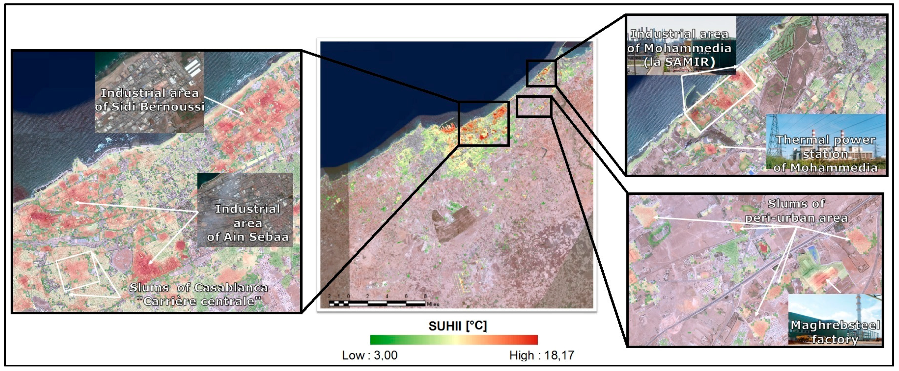
| Industrial areas | 7.03 | 18.17 |
© 2016 by the authors; licensee MDPI, Basel, Switzerland. This article is an open access article distributed under the terms and conditions of the Creative Commons Attribution (CC-BY) license (http://creativecommons.org/licenses/by/4.0/).
Share and Cite
Bahi, H.; Rhinane, H.; Bensalmia, A.; Fehrenbach, U.; Scherer, D. Effects of Urbanization and Seasonal Cycle on the Surface Urban Heat Island Patterns in the Coastal Growing Cities: A Case Study of Casablanca, Morocco. Remote Sens. 2016, 8, 829. https://doi.org/10.3390/rs8100829
Bahi H, Rhinane H, Bensalmia A, Fehrenbach U, Scherer D. Effects of Urbanization and Seasonal Cycle on the Surface Urban Heat Island Patterns in the Coastal Growing Cities: A Case Study of Casablanca, Morocco. Remote Sensing. 2016; 8(10):829. https://doi.org/10.3390/rs8100829
Chicago/Turabian StyleBahi, Hicham, Hassan Rhinane, Ahmed Bensalmia, Ute Fehrenbach, and Dieter Scherer. 2016. "Effects of Urbanization and Seasonal Cycle on the Surface Urban Heat Island Patterns in the Coastal Growing Cities: A Case Study of Casablanca, Morocco" Remote Sensing 8, no. 10: 829. https://doi.org/10.3390/rs8100829