Article

Comparison between the Suomi-NPP Day-Night Band and DMSP-OLS for Correlating Socio-Economic Variables at the Provincial Level in China

1
Department of Astronomy, University of Maryland, College Park, MD 20742, USA
2
School of Earth & Space Sciences, Yaogan Bldg, Peking University, No.5 Yiheyuan Road, Haidian District, Beijing 100871, China
3
NOAA/NESDIS/STAR, College Park, MD 20742, USA
4
School of Economics, Mingde Bldg, Renmin University of China, Beijing 100872, China
*
Author to whom correspondence should be addressed.
Remote Sens. 2016, 8(1), 17; https://doi.org/10.3390/rs8010017
Submission received: 27 November 2015 / Revised: 15 December 2015 / Accepted: 21 December 2015 / Published: 25 December 2015
(This article belongs to the Collection Visible Infrared Imaging Radiometers and Applications)

Abstract

:
Nighttime light imagery offers a unique view of the Earth’s surface. In the past, the nighttime light data collected by the DMSP-OLS sensors have been used as an efficient means to correlate regional and global socio-economic activities. With the launch of the Suomi National Polar-orbiting Partnership (Suomi-NPP) satellite in 2011, the day-night band (DNB) of the Visible Infrared Imaging Radiometer Suite (VIIRS) onboard represents a major advancement in nighttime imaging capabilities, because it surpasses its predecessor DMSP-OLS in radiometric accuracy, spatial resolution and geometric quality. In this paper, four variables (total night light, light area, average night light and log average night light) are extracted from nighttime radiance data observed by the VIIRS-DNB composite in 2013 and nighttime digital number (DN) data from the DMSP-OLS stable dataset in 2012, respectively, and correlated with 12 socio-economic parameters at the provincial level in mainland China during the corresponding period. Background noise of DNB composite data is removed using either a masking method or an optimal threshold method. In general, the correlation of these socio-economic data with the total night light and light area of VIIRS-DNB composite data is better than with the DMSP-OLS stable data. The correlations between total night light of denoised DNB composite data and built-up area, gross regional product (GRP) and power consumption are higher than 0.9 and so are the correlations between the light area of denoised DNB composite data and city and town population, built-up area, GRP, power consumption and waste water discharge. However, the correlations of socio-economic data with the average night light and log average night light of VIIRS-DNB composite data are not as good as with the DMSP-OLS stable data. To quantitatively analyze the reasons for the correlation difference, a cubic regression method is developed to correct the saturation effect of the DMSP stable data, and we artificially convert the pixel value of the DNB composite into six bits to match the DMSP stable data format. The correlation results between the processed data and socio-economic data show that the effects of saturation and quantization are two of the reasons for the correlation difference. Additionally, on this basis, we estimate the total night light ratio between saturation-corrected DMSP stable data and finite quantization DNB composite data, and it is found that the ratio is ~11.28 ± 4.02 for China. Therefore, it appears that a different acquisition time is the other reason for the correlation difference.

Graphical Abstract

1. Introduction

Remote sensing of the environment provides great opportunities to understand links between human and nature and global socio-economic changes. With rapid advances in remote sensing technology and its applications, it becomes increasingly more desirable to use remote sensing data to study and monitor the socio-economic environment. Nighttime light imagery stands distinctly against various remote sensing data sources, as it offers a unique view of the Earth’s surface in the light of human activities. Nocturnal lighting becomes one of the hallmarks of modern development and provides a unique attribute for identifying the presence of development or human activity that can be sensed remotely. The presence of lighting across the globe is mostly due to some form of human activity, such as human settlements, shipping fleets, gas flaring or fire associated with swidden agriculture [1,2].
Satellite sensors, such as OLS on DMSP, have been acquiring day/night images since the early 1970s for applications, such as military surveillance, population estimation, monitoring social-economic development and power consumption and providing weather- and climate-related data [3]. The DMSP-OLS sensor distinguishes itself from the rest of passive, optical remote sensing in that the data can be acquired at night and are sensitive to light sources down to a minimum detectable radiance of 10−9 W/cm2-sr [4,5]. In essence, the radiance detected by the sensor, after masking out clouds using the OLS thermal infrared channel, are mostly man-made light sources, primarily from cities, but also from oil-field gas-flare burn off, biomass burning and shipping fleets [6].
In the past, the remote sensing of nighttime light with DMSP-OLS was actively studied and shown to be an accurate, economical and straightforward way of mapping the global distribution and density of developed areas, as well as population [2]. Night light imagery data were also used in mapping regional economic activity at the national and regional level. Welch [7] showed quantitative relationships between DMSP-OLS nocturnal lighting images of the United States and population, urban area and electric energy utilization patterns. Sutton [8] showed that the correlation between DMSP-OLS data and population density within the urban areas in the United States can be as high as 0.9. Elvidge et al. [9] found that light area estimated from the DMSP-OLS data is highly correlated with gross domestic product (GDP) and electric power consumption. However, significant outliers in the relation between light area and population indicate that it is difficult for DMSP-OLS stable light products to provide direct detection of rural population. Doll et al. [10] developed a method to correlate the light area of a city derived from DMSP-OLS data and statistic data of local socio-economic development to map global economic activity (GDP) and carbon dioxide emissions at the regional level. Elvidge et al. [5] developed a method to perform radiance calibration for the digital number (DN) data of DMSP-OLS. With this method, Doll et al. [11] derived a linear relationship between the intensity of light observed by DMSP-OLS and gross regional product (GRP) for a sub-set of countries within the European Union and U.S. They concluded that different countries have different relationships with total radiance based on their cultures. Sutton et al. [12] developed predictive relationships between observed changes in nighttime satellite images derived from the DMSP-OLS and changes in population and GDP. Letu et al. [13] demonstrated the estimation of electric power consumption from saturated nighttime DMSP-OLS imagery after correction for saturation effects. Additionally, recently, Li et al. [14] used 38 monthly DMSP-OLS System composites covering the period between January 2008 and February 2014 to analyze the response of nighttime light to the Syrian Crisis. The results indicate that the nighttime light experienced a sharp decline as the crisis broke out. Coscieme et al. [15] presented a method based on DMSP-OLS nighttime data that uses nocturnal light data as a proxy measure for the evolution of the non-renewable fraction of national emergy flow. Coscieme et al. [15] found a strict correlation between the intensity of lights and the non-renewable component of national energy flow for more than 100 countries.
One comprehensive study of correlating DMSP-OLS imagery data with multiple socio-economic variables was conducted by Lo [16]. The DMSP-OLS imagery data were acquired between March 1996 and January to February 1997. Lo [16] modeled three types of population parameters (population, non-agricultural population and population density) at the provincial, city and county level in China, respectively, by using four types of variables (light area, percent light area, light volume and pixel mean) derived from OLS imagery data. It was found that the DMSP-OLS nighttime data produced reasonably accurate estimates of non-agricultural population at both the county and city levels using the algometric growth model and the light area or light volume as input. The logarithmic form of the algometric growth model is log P o p u l a t i o n = log a + b log A . Here, a is a coefficient, b is an exponent and A is the built-up area of the settlement. Both a and b are empirically determined. Non-agricultural population density was best estimated using percent light area in a linear regression model at the county level. Lo [16] concluded that the 1-km resolution DMSP-OLS nighttime light image has the potential to provide estimation of the total and urban population of a country from space. Furthermore, Lo [16] presented the relationship between DMSP-OLS imagery data and additional socio-economic parameters at the provincial level in China, such as household, energy consumption, electricity consumption, gross value of industrial output, per capita rural income and per capita urban income. The correlation results between these additional socio-economic parameters and variables derived from the DMSP image were less emphasized in Lo [16] as compared to those obtained with population data.
While the DMSP-OLS is remarkable for its detection of dim lighting, there have been some limitations in DMSP-OLS, such as low spatial resolution (2.7 km ground sample distance), low radiometric resolution (six bit), a saturation effect in bright regions, lack of on-board calibration, lack of systematic recording of in-flight gain changes and lack of multiple spectral bands for discriminating lighting types [2].
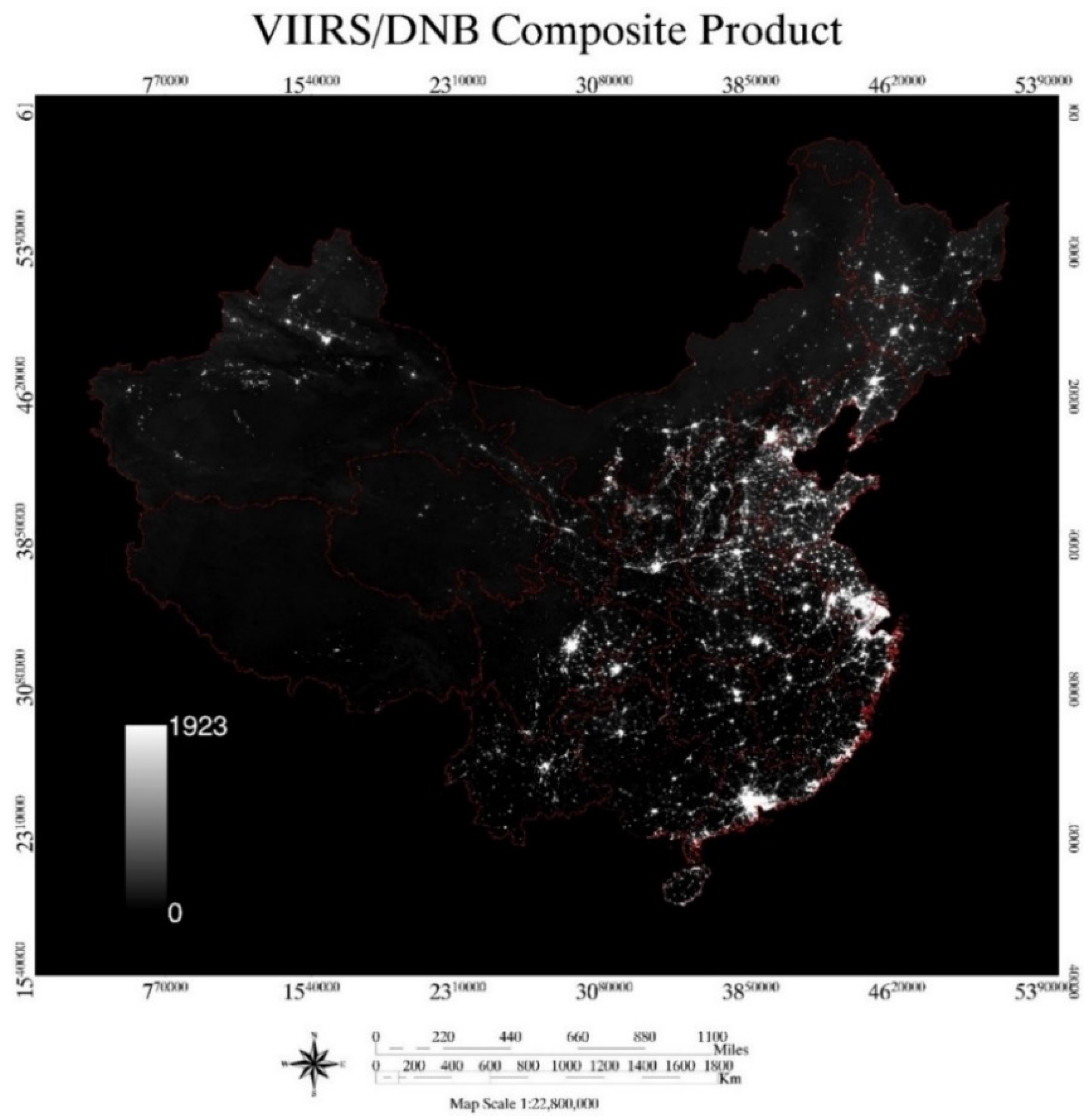
With the launch of the Suomi National Polar-orbiting Partnership (Suomi-NPP) satellite in October 2011, the day-night band (DNB) of the Visible Infrared Imaging Radiometer Suite (VIIRS) onboard represents a major advancement in nighttime imaging capabilities [17,18,19,20,21]. DNB serves primarily to provide imagery of clouds and other Earth features over illumination levels ranging from full sunlight to quarter moon. Other applications of using DNB, such as light outage detections during major storms, have been recently demonstrated [19]. The basic parameters for DNB specifications can be found in Table 1 [22] (Shao et al., 2013). The DNB is a de facto radiometer, because it uses an onboard calibration system to generate the radiances for Earth observations, compared to the DMSP-OLS, which is an imager and has no onboard calibration. The DNB of the VIIRS sensor utilizes a backside-illuminated charge coupled device (CCD) focal plane array (FPA) for sensing of radiances spanning seven orders of magnitude in one panchromatic (0.5 to 0.9 μm) reflective solar band (RSB). In order to cover this extremely broad measurement range, the DNB employs four imaging arrays that comprise three gain stages. The low gain stage (LGS) gain values are determined by solar diffuser data. In operations, the medium and high gain stage values are determined by multiplying the LGS gains by the medium gain stage (MGS)/LGS and high gain stage (HGS)/LGS gain ratios, respectively [23]. The DNB relies on collocation with multispectral measurements on VIIRS and other Suomi-NPP sensors for accurate geolocation. The spatial resolution of the DNB is approximately 750 m across the entire swath. This is achieved by performing on-chip aggregation of the CCD detector elements that form pixels, which results in 32 aggregation zones through each half of the instrument swath on either side of nadir. The aggregation zones near the end of scan (EOS) have fewer pixels than the zones near nadir, as the footprint of a single CCD detector element on the ground is much larger at EOS. These improvements, coupled with the multispectral complementary information from other collocated VIIRS channels, enables the use of Suomi-NPP to pursue quantitative applications heretofore restricted to daytime measurements, a true paradigm shift in nighttime remote sensing capability.
Shi et al. [24] suggested that VIIRS data might be more indicative of demographics and economics than DMSP data at both the city and the province scales by statistically comparing the correlations between nighttime light brightness and socio-economic variables. Ma et al. [25] investigated correlations of DNB nighttime light radiance with GDP, population, electrical power consumption and paved road areas, and this work indicated that these parameters had a significantly positive linear relation with nighttime light radiance. The application of VIIRS DNB nighttime data, beyond correlating with socio-economic data [26,27,28,29,30,31,32], also can be used to detect social insurgency [33].
Table 1. Design specifications for Suomi-National Polar-orbiting Partnership (Suomi-NPP) VIIRS-day-night band (DNB). HGS, high gain stage; MGS, medium gain stage; LGS, low gain stage.
Spectral Band0.5 to 0.9 μm
Relative Radiometric Gains119,000:477:1 (HGS:MGS:LGS)
Dynamic RangeLmax/Lmin = 6,700,000
Number of Bits in analog to digital (A/D)14 bits (16,384 levels) for HGS; 13 bits (8192 levels) for MGS and LGS
Spatial Resolution750 m
Aggregation32 aggregation zones
Time Delay Integration (TDI)1, 3 and 250 pixels for LGS, MGS and HGS, respectively
Number of Samples per Scan4064
Recent work by Li et al. [26] compared the capabilities of using DNB and DMSP-OLS data to model the gross regional product (GRP) in China. One variable, total night light (TNL), is derived from DNB and DMSP imagery data to model GRP at the provincial and county level in China with a linear regression model. It was shown that the TNL derived from Suomi-NPP DNB exhibit R2 values of 0.8699 and 0.8544 when correlating with the provincial and county GRP, respectively, which are significantly better than the correlative relationship between the TNL from DMSP-OLS F16 (0.6923) and F18 (0.7056) satellites and GRP. This demonstrated that the DNB nighttime light imagery has a stronger capability in modeling GRP than those of the DMSP-OLS data. However, the comparison between Suomi-NPP DNB and DMSP-OLS in correlating with regional socio-economic variables performed by Li et al. [26] is limited to correlating one socio-economic parameter, i.e., GRP, with one light variable (total night light) derived from nighttime imagery data. However, Li et al. [26] only gave the three general potential factors (the saturation effect of DMSP-OLS in city centers, the different acquisition time between DNB and DMSP-OLS data and the onboard calibration system on NPP-VIIRS) that make DNB data more efficient than the OLS data in modeling the economy, but without any quantitative analysis. Factors that cause the difference between DNB and DMSP observations in correlating with GRP remain to be investigated.
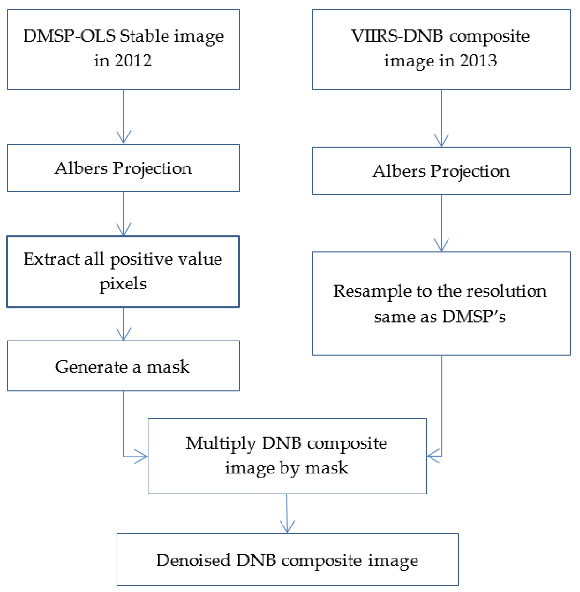
In this paper, we focus on comparing the performance of imagery data of the DMSP-OLS stable data with that of Suomi-NPP DNB composite data in correlating with multiple regional socio-economic parameters in China. We developed methods to remove the background noises that are not related to economic activities in DNB data. Different from the work of Li et al. [26], we calculate correlations between four light variables derived from nighttime imagery data and multiple socio-economic parameters to assess the difference between the DMSP-OLS stable data and the DNB composite data in correlating with socio-economic parameters. In view of the significant differences between DMSP data and DNB, such as different data quantization, the saturation effect of the DMSP stable data and data acquisition time at night, i.e., DNB at ~1:30 a.m. versus DMSP-OLS at ~9 p.m. Equator cross time, we use a cubic regression model to correct the saturation pixels of the DMSP stable data, artificially quantize the pixel value of the DNB composite data into six bit and estimate the ratio of total night radiance between saturation-corrected DMSP-OLS stable and finite quantization DNB composite data for China.
In the following sections, we first introduce the data and regional areas studied in our work. In Section 3, we first illustrate the variables of interest derived from nighttime light data. Then, the noise masking method (NMM) and the optimal threshold method (OTM) are presented for removing background noise of DNB composite data. The correlation results between variables from nighttime data and socio-economic parameters are given. Section 4 explores the factors that contribute to the correlation difference between the DNB composite data and the DMSP-OLS stable data. The conclusion is given in Section 5.

2. Data and Study Area

2.1. Nighttime Imagery Data

In this study, both DMSP-OLS stable data and Suomi-NPP VIIRS DNB composite data over mainland China are used. The VIIRS-DNB (Figure 1) composite data used in this study are the first global cloud-free composite of VIIRS nighttime lights and acquired from the Earth Observation Group (EOG) of NOAA‘s National Geophysical Data Center (NGDC).
Figure 1. The VIIRS-day-night band (DNB) composite data of mainland China in 2013 (multiplying the pixel value by 10−9 gives radiance in units of W/cm2-sr).
Remotesensing 08 00017 g001
These global composite of VIIRS nighttime light data are assembled with observations collected at nights with zero moonlight during the periods of April and October in 2012 and January in 2013. Cloud screening was performed based on the detection of clouds using the observations from the M15 infrared thermal band of VIIRS. However, this data product has not been filtered to remove lights associated with fires, gas flares, volcanoes or aurora. Furthermore, the background noise has not been subtracted [34]. First, we used a mean algorithm to remove the abnormal lights that may be associated with fires and gas flares. Then, we introduced the noise masking method (NMM) and the optimal threshold method (OTM) to remove background noise in DNB composite data, and these methods are illustrated in Section 3.2 and Section 3.3. 2012 composite data reveal significant geolocation issues, which were due to a DNB pointing error or systematic offset in computing the location of nadir. In the nighttime data, this resulted in a westward shift of entire scans, with off-nadir pixels more affected than pixels close to nadir. When making a composite (or average) product, the effect was an enlarged footprint in the track direction of the composite and an average radiance, which was not representative of the ground pixel, as it was an average of a close-by region depending on geolocation accuracy. NOAA/NGDC developed software to correct for these pointing errors, and these errors were fixed in the January 2013 composite. Therefore, we use January 2013 DNB composite data to compare to the DMSP-OLS stable product in this paper. January is not the burn season in China, so the biomass burning effect can be ignored in this month.
The DMSP stable data are also acquired from the NGDC/EOG. This dataset is cloud-free composites assembled using all of the archived smooth resolution data of DMSP-OLS that are available during calendar years. The products are in a spatial resolution of 30 arc seconds [35]. The composite products of DMSP data we use in this study were stable light products and acquired by the F18 satellite in 2012. In this data product, the background noise was identified and replaced with values of zero, and ephemeral events have been discarded, so that only lights from cities, towns and other sites with persistent lighting (including gas flares) remain [36]. All of the nighttime light imagery was re-projected using Albers conical equal-area projection with its original resolution. The details of nighttime light data are described in Table 2.
Table 2. Year and spatial resolution of the satellite imagery data used in this study and the year of the corresponding socio-economic data used to correlate with these imagery data. All of the satellite data are obtained from National Geophysical Data Center (NGDC)/Earth Observation Group (EOG).
YearImagery DataArchived CompositesResampled Imagery in this StudyYear of Socio-Economic Data to Correlate with
2013VIIRS/DNB composite data 15 arc seconds491 m2013
2012DMSP/F18 stable data30 arc seconds982 m2012
In this paper, we assume that the night light distributions in mainland China during the 12-month composite in 2012 and the 1-month composite in 2013 are the same. Then, four types of variables, total night light (TNL), light area (LA), average night light (ANL) and logANL of each administrative region, were derived from nighttime image. Details on these four variables can be found in Section 3.1.

2.2. Socio-Economic Data

In this study, socio-economic parameters chosen to be correlated with nighttime imagery data are acquired from China Statistical Yearbook for Regional Economy, China City Statistical Yearbook, and China Statistical Yearbook. In total, there are 12 socio-economic parameters chosen for correlating in this study. The abbreviations, sources and units of these parameters are described in Table 3.
Table 3. The abbreviations, sources and units of socio-economic parameters at the provincial level used in this study.
Socio-Economic ParametersAbbreviationsUnitSource
Total PopulationTPTen thousandsa
City PopulationCPTen thousandsd1
City and Town PopulationCTPTen thousandsb
HouseholdHH a
City AreaCASquare kmc
Built-up AreaBUASquare kmc
Gross Regional ProductGRPOne hundred million Yuana
GRP Per CapitaGRPPCYuand2
City and Town Per Capita IncomeCTPCIYuanb
Rural Per Capita IncomeRPCIYuanb
Power ConsumptionPWCA hundred million kilowatt hoursb
Waste Water DischargeWWDTen thousand tonsa
a, China Statistical Yearbook; b, China Statistical Yearbook for Regional Economy; c, China City Statistical Yearbook; d1, calculated by multiplying city population density and city area; d2, calculated by dividing GRP by total population.

2.3. Region of Interest and Identification

To evaluate the correlations between socio-economic parameters and night light variables derived from DMSP-OLS and NPP-VIIRS imagery data, we focus on analyzing administrative regions at the provincial level in mainland China. Thirty-one provinces in mainland China are selected for the analysis. Boundary data of these 31 provinces at the scale of 1:4 million in ArcInfo format for year 2000 were obtained from the Data Sharing Infrastructure of Earth System Science [37]. The nighttime imagery data were registered to the corresponding provincial units using ENVI software. Figure 1 illustrates the composite observations by DNB of these 31 provincial regions of mainland China.

3. Methodology and Results

3.1. Variable Extraction from Nighttime Imagery Data

Both the DNB composite data and DMSP stable products are arranged in longitude/latitude format. In our analysis, nighttime image and provincial boundaries are projected using Albers equal-area conic projection available in ArcGIS, which is a conic, equal-area map projection that uses two standard parallels. With this projection, distortion is minimal between the standard parallels. This projection is best suited for land masses extending in an east-to-west orientation.
After applying projection, we extract the pixels and their values within each provincial boundary and derive four variables, total night light (TNL), light area (LA), average night light (ANL) and logANL, which are defined as follows.
Following the approach of Lo [16] and Li et al. [26], the TNL indicates the total amount of light within a given administrative region and is closely related to the socio-economic activities in the region. It is calculated using the following formula:
T N L = L i > L t L i
where L t is the threshold value in mainland China and i is the i-th pixel with a pixel value L > L t . For DMSP-OLS stable data, the pixel value is DN, and the L t is zero. Additionally, for DNB composite data, the pixel value has a radiance unit of W/cm2-sr; the L t is zero when the data have been processed by the noise masking method and is the optimal threshold value when the data have been processed by the optimal threshold method. Each TNL value represents the sum of all pixel values larger than L t in an administrative region. For each kind of nighttime imagery data, we can extract 31 TNL values for the 31 regions, respectively.
As Elvidge et al. [9] and Lo [16] suggested that light area estimated from the nighttime imagery data is highly correlated with socio-economic parameters, we also introduce the light area (LA) as a variable to be extracted from the imagery data, and it is calculated as:
L A = L i > L t A ( L i )
where A is area of the i-th pixel with pixel value L > L t . In this case, the light area is the total area of an administrative region with a pixel value greater than the threshold value L t . Similarly, 31 LA values can be extracted for each kind of nighttime imagery data.
The third variable we extract from the imagery data is average night light (ANL), and it is calculated as:
A N L j = T N L j / L A j
where index j refers to the j-th administrative region and TNLj and LAj are the TNL and LA of region j , respectively, as defined in Equations (1) and (2). Intuitively, ANL can be correlated with per capita-type socio-economic parameters, such as per capita income.
Meanwhile, referencing to the work of Lo [16] and considering the division calculation of the variable ANL, we also introduce the fourth variable logANL in this paper.

3.2. DNB Noise Filtering with the Noise Masking Method

While DMSP-OLS products are stable nighttime data and the background noise and ephemeral lights have been identified and replaced with values of zero [36], the DNB composite data acquired from NGDC have not been filtered to remove light signals associated with fires, gas flares, volcanoes or aurora. In calculating the TNL, LA, ANL and logANL, the key is to remove the dark background noise and ephemeral noises, which are not related to socio-economic activities.
Before removing background noise of the DNB composite, we notice that there are a few outliers of the 2013 DNB composite data in northeast and western China. The outliers are probably caused by lights from the fires of oil or gas flares located in those areas. Since Beijing and Shanghai are the two most developed administrative regions in China, the pixel values of the other areas should not exceed those of the two regions theoretically [29]. The highest radiance of those two regions is 2.62 × 10⁻⁷ W/cm2-sr, and other pixels whose radiance is larger than 2.625 × 10⁻⁷ W/cm2-sr in the DNB composite data were smoothed by their eight neighbors.
After that, this preliminary corrected data also have background noise left. Making reference to the work of Lo [16] and Li et al. [26], we introduce two methods to remove these background noises.
Li et al. [26] developed a simple and approximate method for removing the background noise and ephemeral lights in DNB composite data through applying the mask generated from the 2010 DMSP-OLS stable data to 2012 DNB composite data. It was shown in Li et al. [26] that after applying this method, the correlation of TNL with regional GRP in China is largely increased. By using this method, Li et al. [26] made an assumption that the light areas in the years 2010 and 2012 are the same. During the time of their study, they can only acquire DMSP-OLS stable data in 2010, which is the closest year to 2012. In our work, the DMSP-OLS stable data in 2012 can be acquired, and we can generate a mask from the DMSP-OLS data in 2012, close to the year of DNB composite data. This method is referred as the noise masking method (NMM). Furthermore, we assume that the light areas in the years 2013 and 2012 are the same.
Figure 2. Flow chart of the noise masking method (NMM) in removing background noise for DNB composite data.
Remotesensing 08 00017 g002
Figure 2 shows the flow chart of NMM. Different from the work of Li et al. [26], we use Albers projection in this work instead of the Lambert projection used in Li et al. [26]. The DNB composite data are resampled to the same resolution as that of DMSP-OLS stable light product, i.e., 982 m. Then, we extract all of the pixels with a positive value (DN >0) from 2012 DMSP stable data to generate a mask. The mask is applied to the DNB January 2013 composite imagery data. For pixels outside the mask, the pixel value of DNB data is set as NaN (not a number), and the pixel value is kept the same for pixels inside the mask.

3.3. DNB Noise Filtering with the Optimal Threshold Method

Although NMM can be effective at screening out background noise and ephemeral lights in DNB composite data, this method relies on the DMSP stable data to generate the mask. These masks might not be readily available for the DNB observations of interest and can be outdated as the new DNB observations are made available. Additionally, at the same time, NMM will exclude some small towns and road features that the DNB product is sensitive enough to pick up. Therefore, we introduce another method, the optimal threshold method (OTM), to remove the noises in DNB composite data. To determine the optimal threshold ( L T ), we chose the correlation between LA and built-up area as the object function. The choice of this object function originates from the work by Lo [16] and Chen et al. [38], which showed that light intensity is closely related to the type of land use or land cover and depicts built-up area the best. The object function is defined as:
O ( L t ) = ρ ( L A ( L > L t ) , b )
where ρ ( L A ( L > L t ) , b ) is the correlation coefficient between LA with a pixel value above the intensity threshold value L t and built-up area b ; L t : intensity threshold value;   L A   ( L > L t ) : light areas with a pixel value above the radiance threshold value L t inside administrative regions; b : built-up areas of the regions in China that were acquired from China Yearbook.
The optimal threshold value L T is therefore determined using:
O ( L T ) = max ( O ( L t ) | L t = [ L t 1 ,   L t 2 ] )
so that the resulting correlation O ( L T ) between LA and built-up area reaches the maximum when L t = L T . Here, the light radiance threshold L t varies from L t 1 to L t 2 to determine L T . In our calculation, we use L t 1 equal to 0 and L t 2 equal to 10−7.
Figure 3 illustrates the determination of the optimal threshold value L T from DNB composite data. The X-axis is the radiance value varying from 0 to 10−7 W/cm2-sr. The Y-axis is the correlation coefficient between LA and the built-up area of the provinces of interest. When the correlation coefficient reaches the maximum, the corresponding radiance value is determined as the optimal threshold value L T . As can be seen from Figure 3, the optimal threshold value of the original DNB composite data is determined as L T =   2.15 × 10⁻⁹ W/cm2-sr.
Figure 3. Correlation coefficient between built-up area and light area vs. different threshold values (see Equation (4)) for 31 provinces.
Remotesensing 08 00017 g003
As we will show in Section 3.4.2, OTM is a more effective way than NMM to increase the correlation between LA and socio-economic parameters.

3.4. Correlation Results

We compute TNL, LA, ANL and logANL using Equations (1) to (3) given above for DMSP-OLS stable data and VIIRS-DNB composite data, respectively. For DNB composite imagery data, we applied the NMM and OTM to remove the background noise in composite imagery. The relationships between these variables derived from nighttime imagery and socio-economic parameters are evaluated using the Pearson correlation coefficients.

3.4.1. Correlations with TNL

Table 4 and Figure 4 show the correlation results and scatter plots between TNL and socio-economic parameters, respectively. As shown in Table 4, TNL of DNB composite imagery derived with the NMM and OTM (hereinafter referred to as DNB NMM and DNB OTM, respectively) all have a better correlation with socio-economic parameters than that of TNL-derived from DNB composite imagery without noise filtering. This indicates the importance of noise removal in processing DNB composite data. TNL of DNB NMM has overall better correlation than that derived with OTM. With NMM, The TNL derived from the DNB composite image has correlation coefficients (ρ) with socio-economic parameters all above 0.7. In particular, the correlation of TNL with built-up area (BUA), GPR and power consumption (PWC) are the best, all above 0.9. The correlation of TNL with city population (CP), city and town population (CTP) and waste water discharge (WWD) are relatively in the middle, whose coefficients are 0.85, 0.84 and 0.86, respectively. The correlation of TNL with total population (TP), household (HH) and city area (CA) are relatively weak, but still strong in absolute value, whose coefficients are 0.70, 0.72 and 0.75, respectively.
Comparing the correlation of TNL of the DNB composite image with socio-economic parameters and that of DMSP-OLS stable data, we found that the TNL’s of DNB NMM and DNB OTM in general have a better correlation with most of the socio-economic parameters (except TP and HH) than the correlation derived with DMSP stable data. For TNL from DMSP-OLS stable data, the best correlation is with PWC, whose coefficient is 0.91; the correlations with TP, HH, BUA, GPR and WWD are in the range of 0.8; the correlations with CP, CTP and CA are relatively weak, but still strong in absolute value, whose coefficients are 0.74, 0.79 and 0.70, respectively.
Figure 4 shows the scatter plot of selected socio-economic parameters, such as BUA, GRP and PWC, vs. TNL from DNB NMM, DNB OTM and DMSP-OLS stable data, respectively. It can be seen that Guangdong has the highest BUA and GPR, and Jiangsu has the highest PWC in the year 2013; Guangdong also has the highest BUA, GPR and PWC in the year 2012. Meanwhile, Guangdong has the highest TNL as derived from both DNB NMM (2013) and DNB OTM (2013), and Shandong has the highest TNL as derived from DMSP-OLS (2012) stable data. Xizang has the lowest TNL as derived from both processed DNB composite data and DMSP stable data and has the lowest BUA, GPR and PWC. This suggests that Shandong, Jiangsu and Guangdong provinces are large administrative regions and more industrialized with more night light, which is consistent with the actual situation in China.
Figure 4. Scatter plots of total night light (TNL) vs. socio-economic parameters (1st row: built-up area; 2nd row: gross regional product (GRP); 3rd row: power consumption) together with the fitting curve (in red) from regression. TNL data used in the 1st, 2nd and 3rd column are derived from DNB composite data with NMM, the optimal threshold method (OTM) in 2013 and DMSP-OLS stable data in 2012, respectively. Red labels in the panel denote: GD, Guangdong; SD, Shandong; XZ, Xizang; JS, Jiangsu.
Remotesensing 08 00017 g004
Table 4. Correlation coefficients between TNL and socio-economic parameters. TNL’s are derived from DNB composite data with or without noise filtering and DMSP-OLS F18 stable data, respectively.
DNB TNL 2013DMSP TNL
OriginalNMMOTMF18 2012
TP0.430.700.630.80
CP0.580.850.850.74
CTP0.540.840.810.79
HH0.450.720.660.81
CA0.530.750.730.70
BUA0.670.900.870.86
GRP0.620.900.880.86
PWC0.710.910.870.91
WWD0.570.860.850.80
In summary, applying noise-filtering methods, i.e., NMM or OTM, to DNB composite data helps improve the correlation between TNL and socio-economic parameters. The NMM produces the best performance in correlating TNL of DNB composite data with socio-economic parameters in comparison with another method. The correlation of TNL from DNB NMM is better than that of DMSP stable data for almost all of the parameters, except TP and HH, and that with PWC is comparable. Li et al. [26] studied the correlation only between TNL and GRP, and our results on this correlation are consistent with what they concluded.

3.4.2. Correlations with LA

Table 5 and Figure 5 show the correlation results and scatter plots between LA and socio-economic parameters, respectively.
As shown in Table 5, the LA’s derived from DNB NMM and DNB OTM all have significant better correlations with socio-economic parameters than that of LA derived from the DNB composite without noise filtering. The correlation coefficients of LA derived from DNB OTM are all above 0.77. In particular, the correlations of LA derived from DNB OTM with economic parameters (CTP, BUA, GRP, PWC and WWD) are among the best, all above 0.9. LA of DNB OTM has a much better correlation than that of DNB NMM, particularly in correlating with CP, CTP, CA, BUA, GRP, PWC and WWD. The best correlation of LA derived from DNB NMM has ρ ~ 0.78, i.e., TP and HH, far less than ρ > 0.9 achieved for the correlation of LA using OTM with CTP, BUA, GRP, PWC and WWD. This illustrates that OTM is a more effective way than NMM to remove noisy background of DNB composite data and deriving socio-economic activity-related LA from the data. Therefore, using OTM can more effectively improve the correlative relationship between LA of DNB composite data and socio-economic parameters.
Table 5. Correlation coefficients between LA and socio-economic parameters. LA’s are derived from DNB composite data with or without noise filtering and DMSP-OLS F18 stable data, respectively.
DNB 2013 LADMSP LA
OriginalNMMOTMF18 2012
TP−0.270.780.780.78
CP−0.330.580.860.59
CTP−0.330.720.900.75
HH−0.290.780.800.78
CA−0.270.550.770.54
BUA−0.230.740.930.73
GRP−0.310.680.940.68
PWC−0.160.750.950.75
WWD−0.300.650.920.65
Since the administrative region of interest of DNB NMM data is generated from the DMSP-OLS mask, the correlations of LA using DNB NMM and the DMSP stable data are similar; only the correlations with CP, CTP, CA and BUA have small differences, which is because the years of the corresponding socio-economic data that DNB NMM and DMSP stable data correlated with are different. Therefore, the performances of the correlation of LA derived from both DNB NMM and DMSP-OLS stable data with socio-economic parameters are almost the same.
Figure 5 shows the scatter plot of selected socio-economic parameters, such as household, city and town population and power consumption vs. LA from DNB NMM, DNB OTM and DMSP-OLS stable data, respectively. From Figure 5, Guangdong and Shandong have the largest LA as derived from DNB OTM (2013) and DMSP-OLS stable data (2012), respectively. Xizang has the smallest LA as derived from both DNB denoised data and DMSP-OLS stable data. This relative ranking of LA among Guangdong, Shandong and Xizang is consistent with the ranking of TNL. Correspondingly, Shandong, Guangdong and Jiangsu have the highest household, city and town population and power consumption in the year 2013, respectively, Shandong has the highest HH, and Guangdong has the highest CTP and PWC in the year 2012. Still, Xizang province has the lowest built-up area, GPR and power consumption.
Figure 5. Scatter plots of light areas (LA’s) vs. socio-economic parameters (1st row: household; 2nd row: city and town population; 3rd row: power consumption) together with the fitting curve (in red) from regression. LA data used in the 1st, 2nd and 3rd column are derived from DNB composite with NMM and OTM in 2013 and DMSP-OLS stable data in 2012, respectively. Red labels in the panel denote: GD, Guangdong; SD, Shandong; XZ, Xizang; JS, Jiangsu.
Remotesensing 08 00017 g005
From Table 4 and Table 5, it can also be observed that using OTM in deriving TNL and LA from DNB composite data, the resulting correlations with BUA, GRP, PWC and WWD are all quite strong, i.e., above 0.92 for LA and between 0.85 and 0.88 for TNL. This suggests that OTM is consistent in removing noise for calculating the correlation with both LA and TNL and is an effective method for filtering DNB data to model these socio-economic parameters. Meanwhile, based on the generation procedure of DNB NMM data, its performance for LA in correlating with the parameters is the same as DMSP stable data, but has better performance of TNL than DNB OTM data in correlating with the parameters, especially with BUA, GRP, PWC and WWD (economic parameters).

3.4.3. Correlations with ANL and logANL

Table 6 and Table 7 show the correlation results between socio-economic parameters and both ANL and logANL, respectively. Figure 6 shows scatter plots between logANL and multiple socio-economic parameters. Since the ANL is derived by dividing TNL with LA, it should be related to per-capita socio-economic parameters, such as per capita GRP and per capita income, in evaluating its correlation.
Table 6. Correlation coefficients between ANL and socio-economic parameters. ANL’s are derived from DNB composite data with or without noise filtering and DMSP-OLS stable data, respectively.
DNB ANL 2013DMSP ANL
OriginalNMMOTMF18 2012
GRPPC0.690.710.670.84
CTPCI0.780.810.770.88
RPCI0.770.800.760.89
Table 7. Correlation coefficients between logANL and socio-economic parameters. logANL’s are derived from DNB composite data with or without noise filtering and DMSP-OLS stable data, respectively.
DNB logANL 2013DMSP logANL
OriginalNMMOTMF18 2012
GRPPC0.830.840.750.89
CTPCI0.840.880.790.90
RPCI0.880.870.810.91
Figure 6. Scatter plots of logANL vs. socio-economic parameters (1st row: GRPPC; 2nd row: CTPCI; 3rd row: RPCI) together with the fitting curve (in red) from regression. logANL data used in the 1st, 2nd and 3rd column are derived from original DNB composite data in 2013, DNB NMM in 2013 and DMSP-OLS stable data in 2012, respectively. Red labels in the panel denote: GS, Gansu; GZ, Guizhou; GX, Guangxi; SH, Shanghai; TJ, Tianjin; XZ, Xizang.
Remotesensing 08 00017 g006
Figure 6 shows the scatter plot of the selected socio-economic parameters, such as GRP per capita (GRPPC), CT per capita income (PCI) and RPCI vs. logANL from original DNB composite data, DNB NMM and DMSP-OLS stable data, respectively. As mentioned above, ANL is derived by dividing TNL with LA, so the province with the highest ANL is different from that with the highest TNL and LA. Shanghai has the highest logANL for both DNB composite data and DMSP-OLS stable data. Accordingly, Shanghai also has the highest CTPCI and RPCI over the two years of interest, and Tianjin has the highest GRPPC in both years. On the other hand, Xizang, Guangxi and Guizhou have the lowest logANL for original DNB composite data, DNB NMM data and DMSP-OLS stable data, respectively. Guizhou has the lowest GRPPC, and Gansu has the lowest CTPCI and RPCI in both years. This indicates that Shanghai is more industrialized, has a higher living standard per capita and, therefore, more night light emission in ANL, which is indeed the scenario in China.

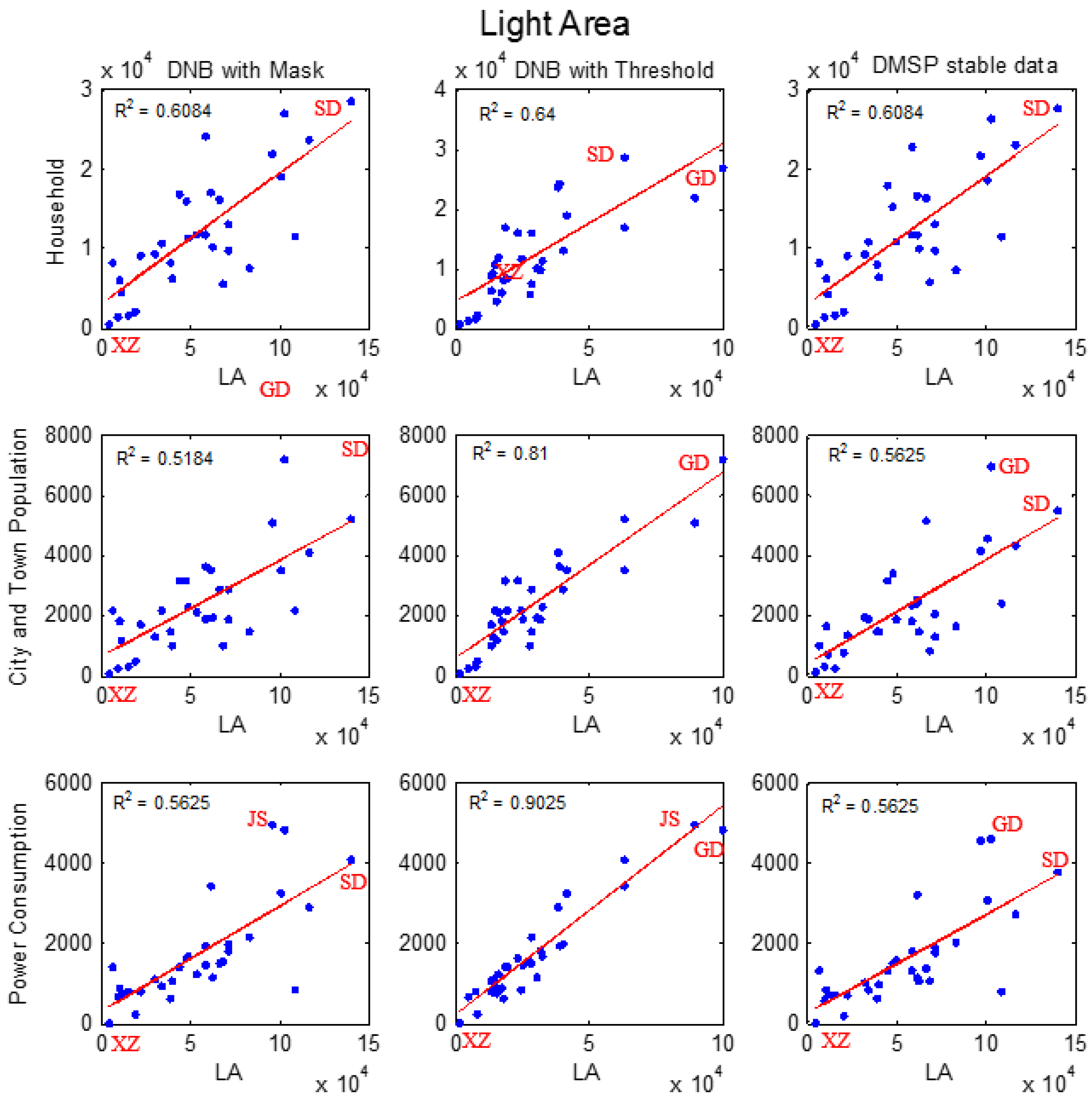
4. Analysis and Discussions
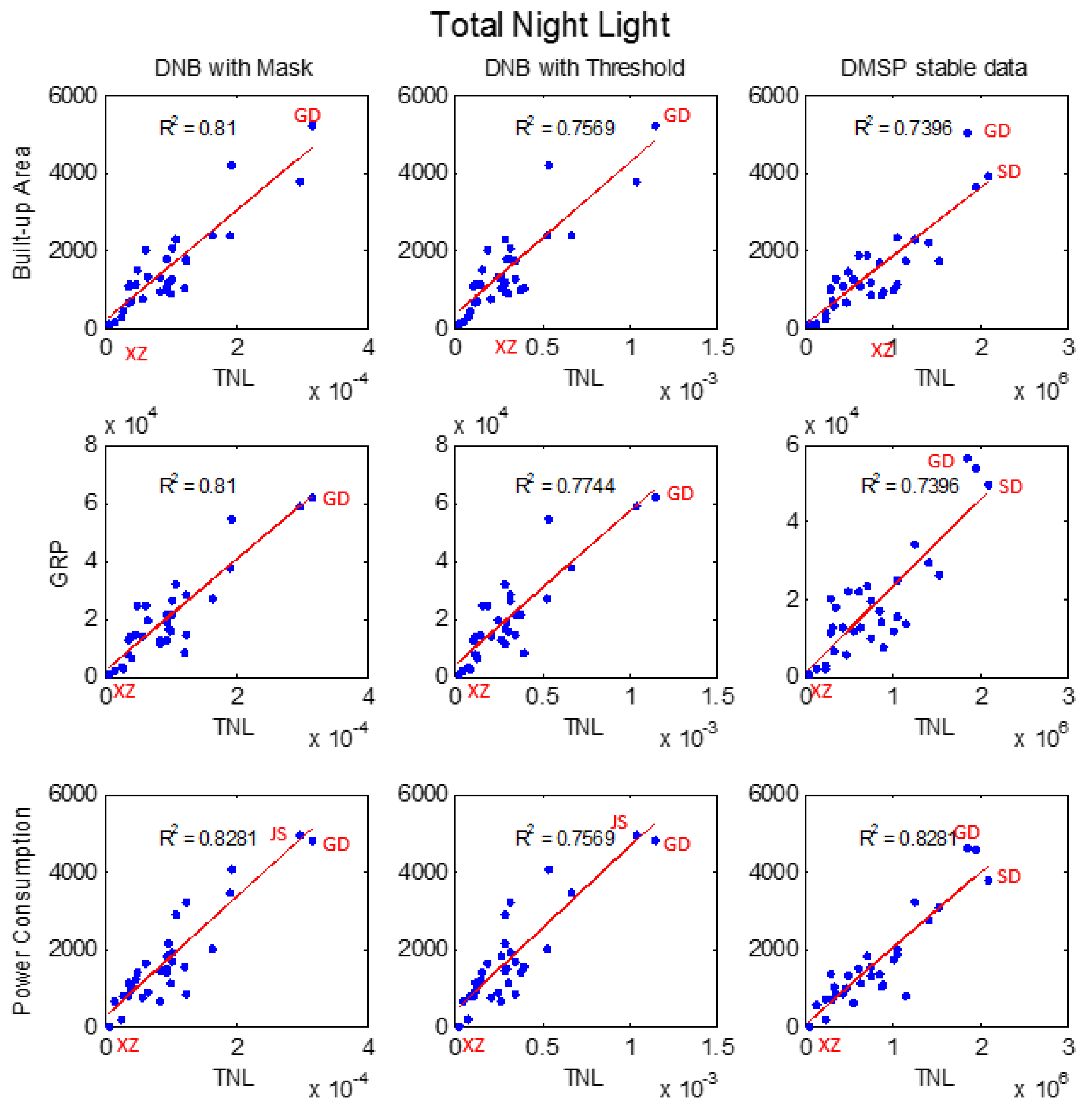
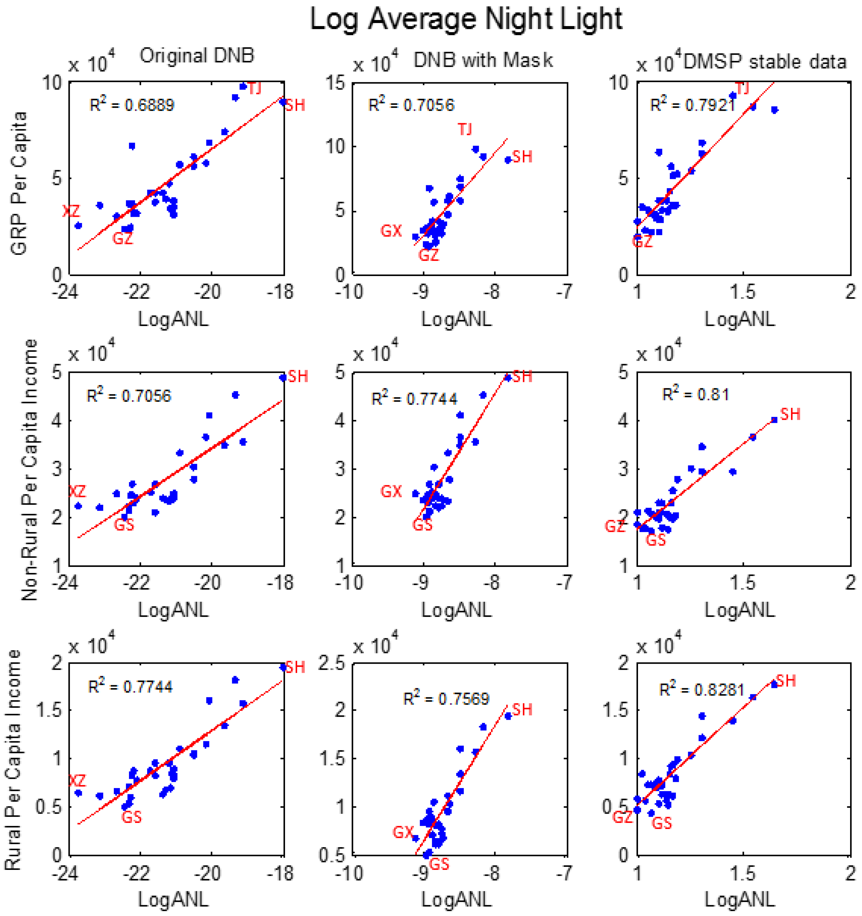
From Section 3.4, it can be seen that the correlation of socio-economic data with the TNL and LA of denoised DNB composite data is in general better than with DMSP-OLS stable data. The correlations with ANL and logANL of DNB composite data are not as good as with DMSP-OLS stable data. Therefore, this section focuses on the cause analysis of the correlation difference with variable TNL. In this section, we analyze the reasons for the correlation difference between DMSP stable data and DNB NMM data, rather than DNB OTM data, because, since the DNB NMM is derived from DMSP stable data, we can pay more attention to the nighttime light intensity difference between DNB composite and DMSP stable data instead of the difference caused by noise removal methods. For the same reason, we will not analyze correlation difference with variables LA, ANL and logANL in this paper.
To find out the factors that cause the correlation difference between DNB NMM and DMSP-OLS stable data, we here analyze the primary difference (Table 8 [5,35]) between DNB composite and DMSP-OLS stable data, such as the effects of the saturation and quantization of the pixel value and the TNL ratio between different nighttime datasets.
Table 8. Main differences between VIIRS-DNB and DMSP-OLS data.
DataSpatial ResolutionPixel ValueSaturation EffectQuantizationAcquisition Time (Local Time)
VIIRS/DNB750 m (Observed) 15 arc second (NGDC)RadianceNO14 bit [39]1:30 a.m.
DMSP-OLS2700 m (Observed) 30 arc second (NGDC)DNYES 6 bit [5]~9 p.m.

4.1. Effect of Saturation

DN data of the DMSP-OLS stable light image can be saturated at centers of city areas where nighttime light is strong [13]. At full spatial resolution (called “fine”), the OLS collects data with a normal pixel size of 0.56 km. Onboard averaging of five by five blocks of fine data produces smoothed data with a ground sampling distance (GSD) of 2.7 km [2]. In this case, saturated and non-saturated fine pixels get averaged together, so the resultant data appears non-saturated [40]. The stable products are made using all of the available archived DMSP-OLS smooth resolution data for calendar years and re-mapped with 1 km × 1 km spatial resolution, so that the sub-pixel saturation phenomenon is not as obvious as the smoothed data. Meanwhile, China is a developing country, and the percentages of saturation area (areasaturation/areapixel value>0) in administrative regions are small (the largest three percentage regions are Beijing, Shanghai and Tianjin, whose saturation area percentages are 0.182, 0.048 and 0.023, respectively). Therefore, we determine that the sub-pixel saturation effect is negligible in this work.
Letu et al. [13] developed a correction method for the saturation light by using a cubic regression equation in the power supply areas in Japan, China and other countries in Asia. The correlation results between cumulative DNs and electric power consumption of each prefecture in China increases after the correction for the saturation DMSP stable light. In this paper, we follow the correction method of Letu et al. [13] to estimate the total DN values in the saturation areas and assess the effect of saturation on the correlation difference.
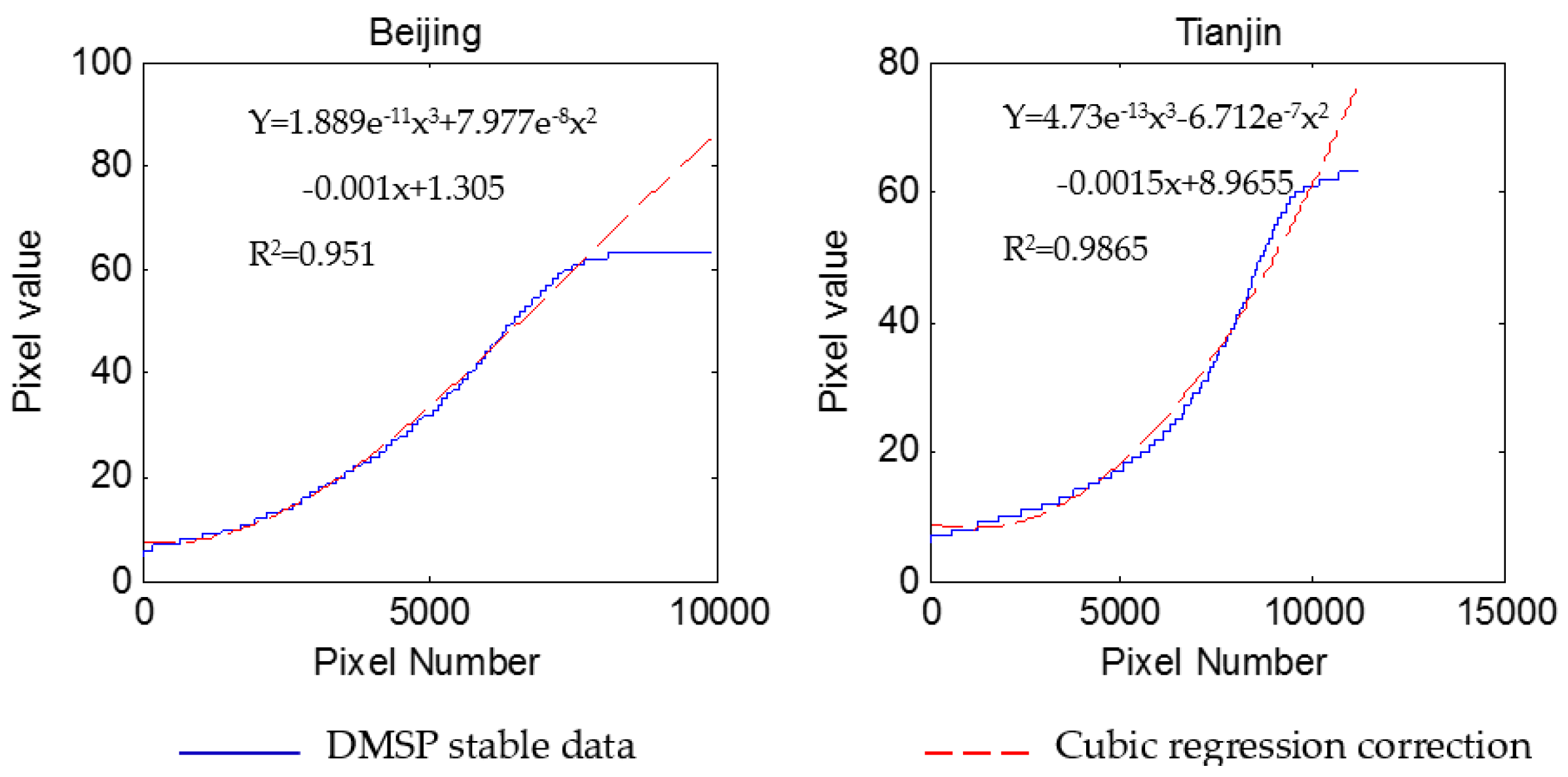
The cubic regression equation is based on the tendency of DN change in non-saturated areas to correct the saturation effect. The cubic regression equation is [13]:
D N T = D N N S + A B ( a x 3 + b x 2 + c x + d )
where D N T is the corrected total DN of the administrative region, D N N S is the total DN of the non-saturation area and A and B are the lower and upper limits of the total number of pixels in the saturation area, respectively. Additionally, a , b , c , d are coefficients that were obtained from a four-dimensional simultaneous equation on the least-squares method.
The correlation results between socio-economic parameters and TNL derived from the saturation-corrected DMSP-OLS stable data are listed in Table 9, and even though the correlation difference from that of TNL derived with DMSP-OLS stable data, Δ ρ , differs at the third decimal point, all of the correlations with saturation corrected data have been improved. This indicates that this cubic regression saturation correction method is effective, and the saturation effect of DMSP stable data is one of the reasons for the correlation difference.
Table 9. Correlations between socio-economic parameters and TNL of DMSP stable data, TNL of saturation-corrected DMSP stable data, TNL of DNB NMM and TNL of DNB NMM after quantization. Δ ρ : difference in the comparison with the correlation derived from TNL of DMSP stable data and DNB NMM, respectively.
TNL of DMSP Stable DataTNL of DNB NMM Data
OriginalSaturation CorrectedOriginalQuantization
Δ ρ Δ ρ
TP0.8010.8080.0070.6950.684−0.011
CP0.7380.7470.0090.8500.8600.010
CTP0.7890.7970.0080.8410.8440.003
HH0.8090.8160.0070.7210.710−0.011
CA0.7000.7090.0090.7540.7560.002
BUA0.8640.8700.0060.9040.898−0.006
GRP0.8560.8650.0090.8990.9100.011
PWC0.9110.9170.0060.9060.9090.003
WWD0.7990.8080.0090.8610.8770.016
Figure 7 shows the correction results for the saturation pixels in Beijing and Tianjin. The correction data vary considerably from the DN of the non-saturated area, and therefore, we could estimate the DN of the saturation areas.
Figure 7. Correction of the saturation light by the cubic regression equation of Beijing and Tianjin, respectively.
Remotesensing 08 00017 g007

4.2. Effect of Quantization

The radiometric signals observed by the DNB sensor are digitized using 14 bits for the HGS and 13 bits for the MGS and LGS. The fine quantization of HGS enhances the appearance of terrestrial light emissions, including faint city lights. By applying gain coefficients and offsets, raw data from DNB observation are converted into radiometric units, i.e., W/cm2-sr [19]. On the other hand, the pixel value of DMSP-OLS stable data obtained from NGDC is of a digital number (DN) in six-bit format with a value between zero and 63.
Fourteen bit and six bit are different in quantization steps. There are more gray levels for 14-bit data compared to six-bit DMSP stable data, so the different quantization might affect the correlation results. Since there is no absolute radiometric calibration for the DMSP-OLS observation in 2012, in this subsection, we show the relationship between the DN value and the radiance of DMSP-OLS stable data firstly. Based on this premise, to study the effect of finite quantization embedded in the DMSP stable data on the performance of correlations with socio-economic parameters, we artificially transform the radiance value of DNB NMM data into six-bit format to match the DN value of the DMSP-OLS stable data format and then compare the resulting correlations.
The DMSP-OLS stable data are acquired under operational conditions, and the gain is varied both along each scan line and as the satellite follows its polar orbit. However, the gain is not recorded in the data stream [40]. In this work, we assume that the gain of the operational stable light product, which is taken by sensors set at the variable, but highest level of gain [41], is fixed (i.e., 55) [40].
The instrument gain of DMSP-OLS is a setting that determines how the detector converts the radiance into a digital number. The transform equation is [40,42]:
D N = D N m a x ( R / R s a t )
where DN is the digital number of the DMSP-OLS data and R is the corresponding radiance. DNmax is 63, and Rsat is the saturation radiance of the detector. Additionally, the following equation gives the relationship between gain setting (G) and saturation radiance:
log 10 R s a t ( C + G ) / 20
where C is a constant coefficient of the relationship between gain and saturation that can be acquired from a pre-launch calibration graph and is subject to change as the instrument degrades. The unit of Rsat is W/cm2/sr. Even though the constant coefficient C for the DMSP-OLS F18 sensor is unreachable, based on the assumption mentioned above and Equations (7) and (8), we can get that the relationship between DN of a specific DMSP-OLS stable dataset, and its corresponding radiance value is linear.
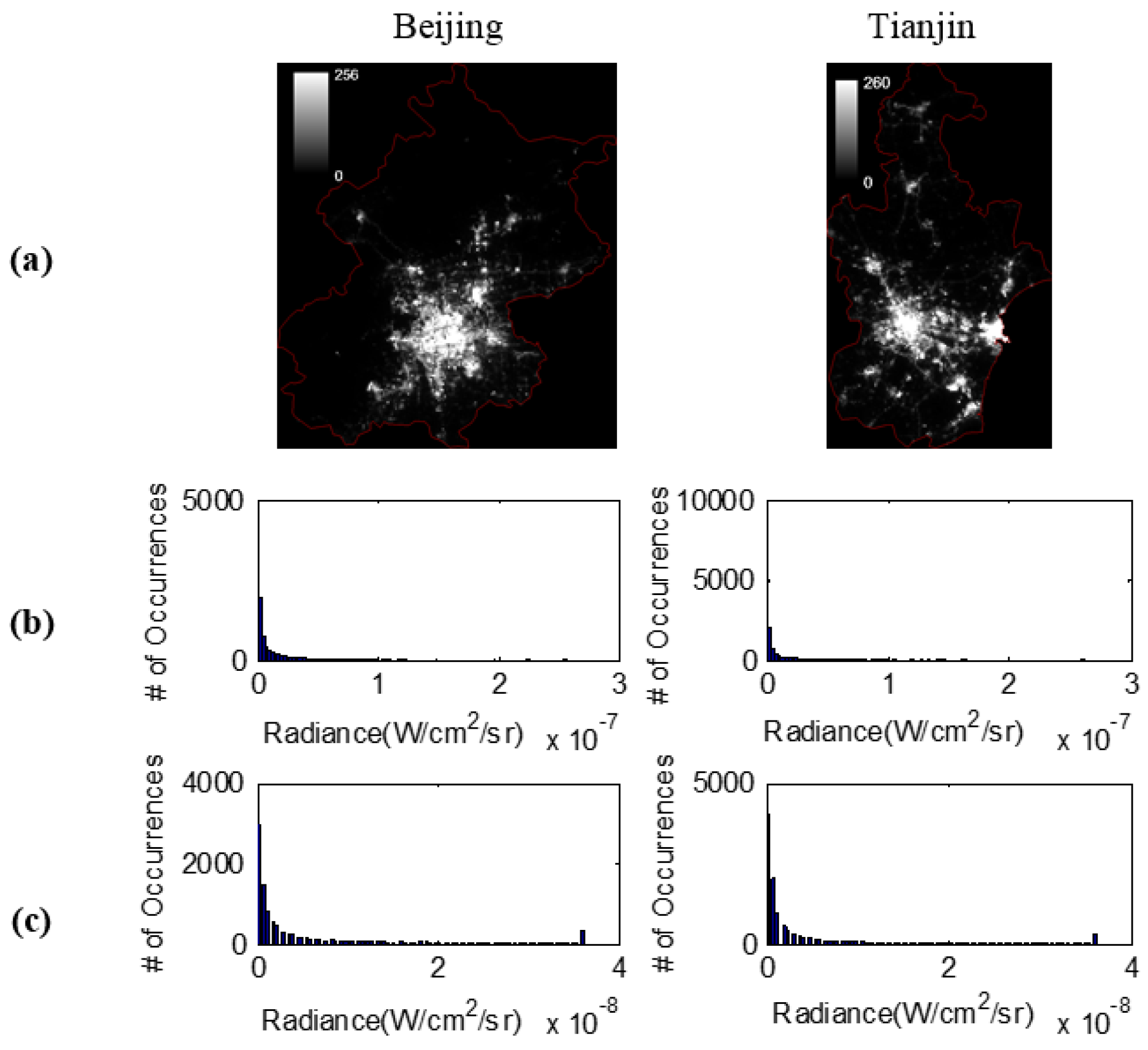
After that, we should find the radiance range of DNB NMM data that will be quantized. We started with the hypothesis that the distribution of the composite night light in China is stable in the years 2012 and 2013, so that the brightness levels of DNB NMM data and DMSP stable data are the same. Therefore, if the DNB composite data have been artificially saturated, the saturated pixel percentage is the same as that of DMSP stable data in China mainland. Then, we arrange the pixels of DMSP stable data and DNB NMM data with a DN value in a gradually increasing order, determine the corresponding radiance value for the saturated DN of DNB composite data, i.e., Lsat = 3.606 × 10⁻⁸ W/cm2-sr, and set pixel values of DNB NMM data larger than Lsat equal to Lsat. Then, we perform an inverse transformation of Equation (7) so that the radiance data from DNB NMM data can be converted to six-bit format to match the DMSP stable data format.
Figure 8 shows the histograms of DNB NMM data transformed with finite quantization for Beijing and Tianjin. Table 9 lists the correlation coefficients between socio-economic parameters and TNL of DNB NMM data after quantization. From Table 9, we notice that, after quantization processing of DNB NMM, the correlations of CP, GRP and WWD have improved compared to the original DNB NMM correlations. Meanwhile, quantization processing makes the correlations with TP, HH and BUA worse. Therefore, the effect of quantization on the correlation difference is noticeable, but socio-economic parameter dependent.
Figure 8. (a) DNB imagery derived with NMM for Beijing (left) and Tianjin (right); (b) histograms of DNB NMM data; (c) histograms of DNB NMM data transformed with finite quantization for Beijing (left) and Tianjin (right), respectively.
Remotesensing 08 00017 g008

4.3. Fluctuation of the TNL Ratio

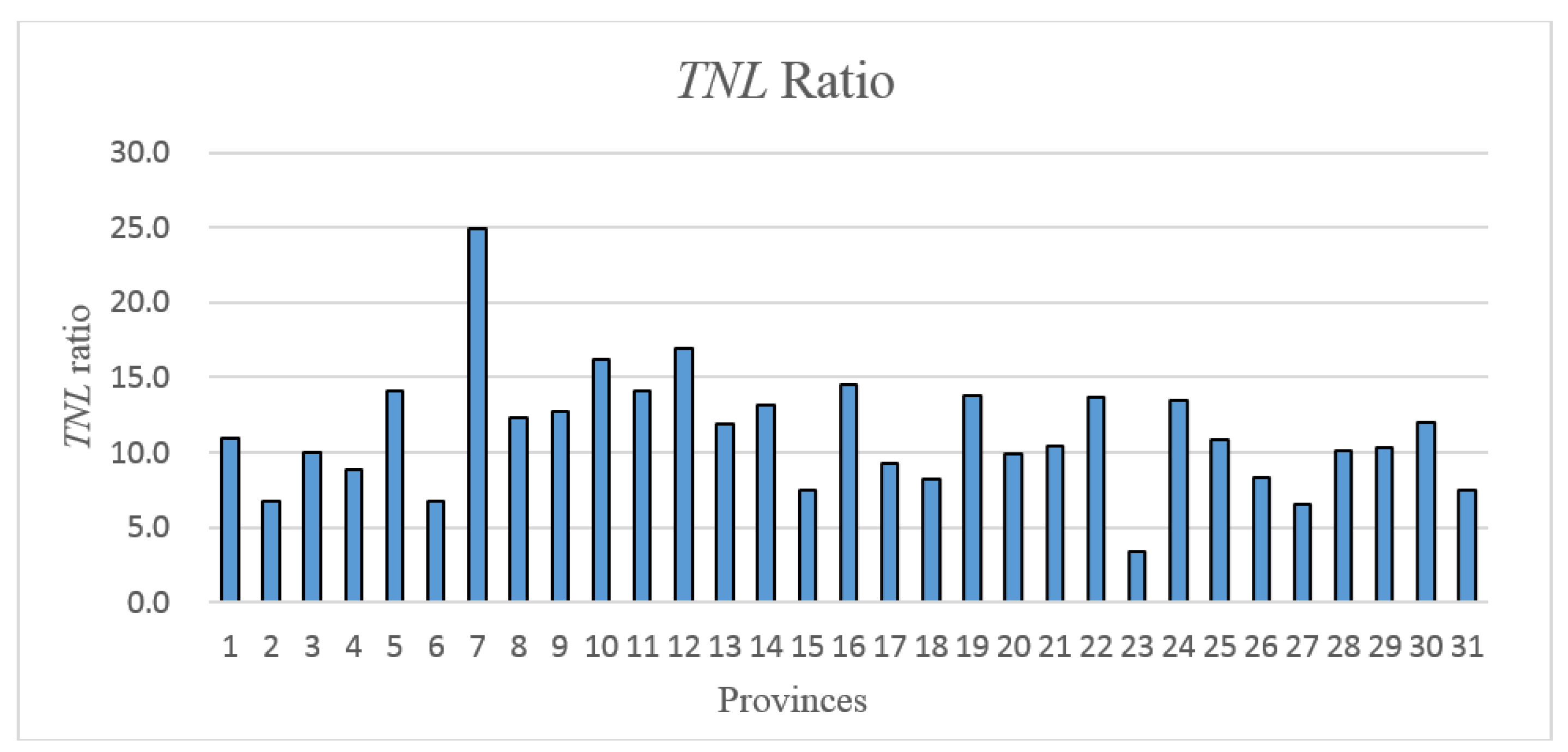
In this sub-section, we compare the difference in the TNL of saturation-corrected DMSP stable data and finite quantization DNB NMM data and finite quantization DNB NMM data for individual provinces. For comparison‘s sake, we calculate the TNL ratio using the pixel value of DNB NMM data instead of the radiance value, and multiplying the pixel value by 10−9 gives radiance in units of W/cm2-sr.
The TNL ratio for 31 provinces derived from the saturation-corrected DMSP stable data in 2012 and quantized DNB NMM data in 2013 ranges from 3.4 to 24.9. The mean of the ratio is ~11.28 ± 4.02. Figure 9 shows the TNL ratio for 31 provinces. This indicates that the fluctuation of these ratios in Figure 9, other than saturation and quantization effects, is the other reason for the correlation difference between DNB composite data and DMSP-OLS stable data. From Figure 9, for provinces that have a large built-up area and are well industrialized, such as Beijing (2), Guangdong (6), Jiangsu (15), Shanghai (23), Tianjin (27) and Zhejiang (31), their TNL ratios are relatively small. For provinces that are relatively underdeveloped, such as Gansu (5), Guangxi (7), Henan (12), Jiangxi (16), Neimenggu (19) Ningxia (22) and Yunnan (30), their TNL ratios are larger.
Figure 9. TNL ratio between saturation-corrected DMSP stable data and quantized DNB composite data for 31 provinces in China. Names corresponding to the indices of these provincial regions are listed in Table A1. Mean ratio = 11.28 and standard deviation of the ratio = 4.02.
Remotesensing 08 00017 g009
DMSP satellites operate in Sun-synchronous orbits with nighttime overpassing at local time from 7 p.m. to 9 p.m. [2]. Additionally, the Suomi-NPP satellite was placed into Sun-synchronous orbit with local equatorial crossing times at ~1:30 a.m. during the nighttime [18]. Because of their different observation times, the characteristics of observed radiance data are quite different. At 1:30 a.m., people are asleep, and residential light sources and light emitted from vehicles are reduced, but the commercial and city infrastructure light sources are still on. Therefore, the reason for the phenomenon of the TNL ratio fluctuation is mainly because of the different data acquisition times. In the well-industrialized regions, commercial and city infrastructure lights are still on at midnight, so the light intensity changes are relatively small at night and midnight. On the contrary, the night light intensity has larger variation in the underdeveloped regions at night and midnight.
We note the different instantaneous field of views (IFOV) and spectral responses will affect TNL; but, for the TNL ratio, the IFOV and spectral response difference will be a constant factor, and the ratio fluctuation tendency will not change. However, still, these ratios only serve as a preliminary and rough estimate for the difference in the nighttime light emission at different night times, i.e., at ~8 p.m. vs. at ~1:30 a.m., in different provincial regions. Other factors, such as saturation correction and finite quantization uncertainty, different data collection times in the year and sensor calibration, etc., can certainly contribute to the overall uncertainty of the ratio estimation.
We use a nearest-neighbor model to resample DMSP stable data to the same spatial resolution as DNB composite data, and its TNL is four times the original DMSP stable data. This will not change the correlation results between DMSP stable data and statistics.
Therefore, the reasons that caused the correlation difference between nighttime data can be the effects of the saturation and quantization of DMSP stable data, and a different acquisition time is another reason for the correlation difference.

5. Conclusions

In this paper, we calculate the correlations between four variables (TNL, LA, ANL and logANL) derived from nighttime light data and 12 socio-economic parameters at the provincial level in mainland China to compare the performance of Suomi-NPP VIIRS/DNB composite data and DMSP-OLS stable data in correlating with regional socio-economic parameters. The noise masking method and optimal threshold method have been used to remove the background noise of DNB composite data that is not related to economic activities before calculating the correlations.
From the correlation results, we can find that the OTM is effective at noise removal for both TNL and LA variables of DNB composite data, and the NMM is effective at noise removal for TNL of DNB composite data. Quantitatively, the correlations between TNL of DNB NMM and BUA, GRP and PWC are higher than 0.90. Additionally, for the LA, OTM can improve the correlations significantly. Correlations between LA of DNB OTM and CTP, BUA, GRP, PWC and WWD are higher than 0.9. For the ANL and logANL, the processing of DNB composite data with NMM and OTM has little effect on the correlations in comparison to the original DNB composite data. All of the results demonstrate that OTM is consistent at removing noise and is an effective method for filtering DNB composite data to model these socio-economic parameters. In addition, from an application perspective, OTM is not bounded by time, but the NMM depends on the masks derived from DMSP stable data of the most recent years.
A comparison is also performed of the relationship between DNB composite and DMSP-OLS stable data with socio-economic parameters through correlation analysis. TNL and LA of DNB composite data have a better correlation than DMSP-OLS stable data in general. For TNL, DNB NMM has a better correlation with all of the socio-economic parameters (except TP and HH) than the correlation derived with DMSP/F18 stable data. For LA, DNB OTM has a better correlation with all of socio-economic parameters than the correlation derived with DMSP/F18 stable data. However, the correlation between ANL/logANL and DNB composite data is not as good as DMSP stable data.
To analyze the factors contributing to the correlation difference between DNB composite data and DMSP stable data, we studied the effects of the differences in their saturation effect, quantization, spatial resolutions and the TNL ratios. A cubic regression method is developed to correct the saturation effect of DMSP stable data. Additionally, we artificially convert DNB composite data into a six-bit value to match the DMSP stable data format. The correlation results between the processed data and socio-economic data show that the effects of saturation and finite quantization are two reasons for the correlation difference. Additionally, on this basis, we estimate the TNL ratio between saturation-corrected DMSP stable data and finite quantization DNB composite data, and it is found that the ratio is ~11.28 ± 4.02 for China. Based on the characteristic of the TNL ratio fluctuation, the fluctuation tendency of the ratio is mainly due to different acquisition times: DMSP and Suomi-NPP satellites overpass at local time about 8 p.m. and 1:30 a.m., respectively. At 1:30 a.m., residential and vehicle light sources are reduced, but commercial light sources are left. The fluctuation tendency consists of the situation in which the night light intensity in more developed regions changes less at night and midnight (Figure 9). That means that the social economic parameters we considered, which have a good correlation with the VIIRS-DNB composite, are indicators of human-related activity. This does not mean that these activities cease when humans are asleep. This means that societal development, city infrastructure and, consequently, light emissions are all correlated.
Note that the ratio of TNL between DMSP-OLS stable and DNB composite data is a rough estimate and can be affected by other factors, such as saturation correction and finite quantization uncertainty, different data collection times in the year, sensor calibration, etc.
In this paper, the VIIRS DNB composite, like some eliminated ephemeral events in OTM, has no further removal, and some faint sources of VNIR emissions have been removed wrongly. These are the next steps of our work about the nighttime light.
The Suomi-NPP VIIRS/DNB is a major step forward from DMSP-OLS in its night-imaging capabilities. The advantages of the DNB sensor are clear: higher radiometric accuracy, finer spatial resolution and higher geometric quality. Additionally, and more importantly, the radiometric data are more reliable and inter-comparable due to the on-board calibration process and three-gain stage of DNB, which ensures no saturation effect at night. The comparison results in this paper confirm this and show that with DNB data, we can quantitatively determine the regional night light in radiance units and assess the correlation with socio-economic parameters. Additionally, our study demonstrates the promising aspects of applying well-calibrated VIIRS-DNB data to estimate long-term regional socio-economic development. With the effort from NOAA to improve the calibration of VIIRS DNB products, it is anticipated that the VIIRS nighttime lights will enable advances in more applications of nighttime imaging products.

Acknowledgments

This study is partially funded by the Joint Polar Satellite System (JPSS) program. The manuscript contents are solely the opinions of the authors and do not constitute a statement of policy, decision or position on behalf of NOAA or the U.S. government.

Author Contributions

Xin Jing, Xi Shao and Changyong Cao conceived of and designed the experiments. Xin Jing and Xi Shao performed the experiments. Xin Jing and Xi Shao analyzed the data. Xin Jing, Xiaodong Fu and Lei Yan contributed auxiliary data. Xin Jing and Xi Shao wrote the paper. Changyong Cao and Lei Yan edited and revised the paper.

Conflicts of Interest

The authors declare no conflict of interest.

Appendix A

Table A1. Socio-economic parameters during 2013 for 31 provinces in mainland China (units and abbreviations for these socio-economic parameters are listed in Table 3).
Index NumberAbbreviationsTPCPCTPHHCA
Anhui1AH60301380288616,1555852
Beijing2BJ211518261825616612,187
Chongqing3CQ29701133173390716134
Fujian4FJ37741105229311,3404299
Gansu5GS2582568103662801450
Guangdong6GD10,6444947721227,05016,136
Guangxi7GX4719942211511,8096104
Guizhou8GZ3502623132592961828
Hainan9HN89524647220601265
Hebei10HB73331608352819,0366478
Heilongjiang11HLJ38351361220111,5542766
Henan12HN94132321412323,6444658
Hubei13HB57991841316115,9077349
Hunan14HN66911430320916,9354312
Jiangsu15JS79392884509022,00814,308
Jiangxi16JX4522960221010,7302113
Jilin17JL27511127149182063596
Liaoning18LN43902324291713,10613,974
Neimenggu19NMG2498885146675218356
Ningxia20NX65426434016842106
Qinghai21QH5781642801414560
Shandong22SD97332945523228,63821,635
shanghai23SH24152415216483776341
Shanxi24SX36301057190899032999
Shaanxi25SAX3764862193110,2031555
Sichuan26SC81071866364024,1366433
Tianjin27TJ1472664120745152334
Xinjiang28XJ2264706100756341620
Xizang29XZ3126274636339
Yunnan30YN4687806189711,7393337
Zhejiang31ZJ54981998351917,03410,992
BUAGRPGRPPCCTPCIRPCIPWCWWD
Anhui17771903931,57425,00680981528266,234
Beijing13061950192,20145,27418,338913144,580
Chongqing11151265742,61526,8508332813142,535
Fujian12632176057,65733,38311,1841701259,098
Gansu727626824,27620,1495108107364,969
Guangdong52326216458,40336,50411,6694830862,471
Guangxi11541437830,46825,02967911238225,303
Guizhou695800722,86321,4135434112693,085
Hainan296314635,15624,920834323236,156
Hebei17872830138,59524,14391023251310,921
Heilongjiang17581438337,50421,1499634845153,090
Henan22893215634,16123,68784752899412,582
Hubei20072466842,53925,18188671630294,054
Hunan15052450236,61924,64383721423307,227
Jiangsu38105916274,52035,13113,5984957594,359
Jiangxi11511433931,70822,9498782947207,138
Jilin13441298147,18823,5449621654117,703
Liaoning23862707861,68027,90510,5232008234,508
Neimenggu12061683267,38326,97885962182106,920
Ningxia421256539,22123,767693181138,528
Qinghai157210136,35022,131619667621953
Shandong41875468456,18430,62810,6204083494,570
shanghai9992160289,45048,87919,5951411222,963
Shanxi10411260234,71724,01471541832138,030
Shaanxi9151604542,62824,10965031152132,169
Sichuan20582626132,39323,89478951949307,648
Tianjin7471437097,62335,65615,84177484,210
Xinjiang1065836036,92722,38872971540100,720
Xizang12080825,88722,5616578315005
Yunnan9361172125,00724,69861411460156,583

References

  1. Doll, C.N.H. CIESIN Thematic Guide to Night-Time Lights Remote Sensing and Its Applications; The Trustees of Columbia University: New York, NY, USA, 2008. [Google Scholar]
  2. Elvidge, C.D.; Erwin, E.H.; Baugh, K.E.; Ziskin, D.; Tuttle, B.T.; Ghosh, T.; Sutton, P.C. Overview of DMSP nightime lights and future possibilities. In Proceedings of the 2009 Joint Urban; Remote Sensing Event, Shanghai, China, 20–22 May 2009; pp. 1–5.
  3. Elvidge, C.D.; Cinzano, P.; Pettit, D.R.; Arvesen, J.; Sutton, P.; Small, C.; Nemani, R.; Longcore, T.; Rich, C.; Safran, J.; et al. The Nightsat mission concept. Int. J. Remote Sens. 2007, 28, 2645–2670. [Google Scholar] [CrossRef]
  4. Elvidge, C.D.; Baugh, K.E.; Kihn, E.A.; Kroehl, H.W.; Davis, E.R. Mapping city lights with nighttime data from the DMSP Operational Linescan System. Photogramm. Eng. Remote Sens. 1997, 63, 727–734. [Google Scholar]
  5. Elvidge, C.D.; Baugh, K.E.; Dietz, J.B.; Bland, T.; Sutton, P.C.; Kroehl, H.W. Radiance calibration of DMSP-OLS low-light imaging data of human settlements. Remote Sens. Environ. 1999, 68, 77–88. [Google Scholar] [CrossRef]
  6. Croft, T.A. Nighttime images of the earth from space. Sci. Am. 1978, 239, 86–98. [Google Scholar] [CrossRef]
  7. Welch, R. Monitoring urban population and energy utilization patterns from satellite data. Remote Sens. Environ. 1980, 9, 1–9. [Google Scholar] [CrossRef]
  8. Sutton, P. Modeling population density with night-time satellite imagery and GIS. Comput. Environ. Urban Syst. 1997, 21, 227–244. [Google Scholar] [CrossRef]
  9. Elvidge, C.D.; Baugh, K.E.; Kihn, E.A.; Kroehl, H.W.; Davis, E.R.; Davis, C.W. Relation between satellite observed visible-near infrared emissions, population, economic activity and electric power consumption. Int. J. Remote Sens. 1997, 18, 1373–1379. [Google Scholar] [CrossRef]
  10. Doll, C.N.H.; Muller, J.P.; Elvidge, C.D. Night-time imagery as a tool for global mapping of socioeconomic parameters and greenhouse gas emissions. Ambio 2000, 29, 157–162. [Google Scholar] [CrossRef]
  11. Doll, C.N.H.; Muller, J.P.; Morley, J.G. Mapping regional economic activity from night-time light satellite imagery. Ecol. Econ. 2006, 57, 75–92. [Google Scholar] [CrossRef]
  12. Sutton, P.C.; Elvidge, C.D.; Ghosh, T. Estimation of gross domestic product at sub-national scales using nighttime satellite imagery. Int. J. Ecol. Econ. Stat. 2007, 8, 5–21. [Google Scholar]
  13. Letu, H.; Hara, M.; Yagi, H.; Naoki, K.; Tana, G.; Nishio, F.; Shuhei, O. Estimating energy consumption from night-time DMPS/OLS imagery after correcting for saturation effects. Int. J. Remote Sens. 2010, 31, 4443–4458. [Google Scholar] [CrossRef]
  14. Li, X.; Li, D. Can night-time light images play a role in evaluating the syrian crisis? Int. J. Remote Sens. 2014, 35, 6648–6661. [Google Scholar] [CrossRef]
  15. Coscieme, L.; Pulselli, F.M.; Bastianoni, S.; Elvidge, C.D.; Anderson, S.; Sutton, P.C. A thermodynamic geography: Night-time satellite imagery as a proxy measure of emergy. Ambio 2013, 43, 1–11. [Google Scholar] [CrossRef] [PubMed]
  16. Lo, C.P. Modeling the population of china using DMSP operational linescan system nighttime data. Photogramm. Eng. Remote Sens. 2001, 67, 1037–1048. [Google Scholar]
  17. Lee, T.E.; Miller, S.D.; Turk, F.J.; Schueler, C.; Julian, R.; Deyo, S.; Dills, P.; Wang, S. The NPOESS VIIRS day/night visible sensor. Bull. Am. Meteorol. Soc. 2006, 87, 191–199. [Google Scholar] [CrossRef]
  18. Miller, S.D.; Mills, S.P.; Elvidge, C.D.; Lindsey, D.T.; Lee, T.F.; Hawkins, J.D. Suomi satellite brings to light a unique frontier of nighttime environmental sensing capabilities. Proc. Natl. Acad. Sci. USA 2012, 109, 15706–15711. [Google Scholar] [CrossRef] [PubMed]
  19. Cao, C.; Shao, X.; Uprety, S. Detecting light outages after severe storms using the S-NPP/VIIRS day/night band radiances. IEEE Geosci. Remote Sens. Lett. 2013, 10, 1582–1586. [Google Scholar] [CrossRef]
  20. Cao, C.; de Luccia, F.J.; Xiong, X.; Wolfe, R.; Weng, F. Early on-orbit performance of the visible infrared imaging radiometer suite onboard the suomi national polar-orbiting partnership (S-NPP) satellite. IEEE Trans. Geosci. Remote Sens. 2014, 52, 1142–1156. [Google Scholar] [CrossRef]
  21. Liao, L.B.; Stephanie, W.; Steve, M.; Bruce, H. Suomi NPP VIIRS day-night band on-orbit performance. J. Geophys. Res. Atmos. 2013, 118, 12705–12718. [Google Scholar] [CrossRef]
  22. Shao, X.; Cao, C.; Uprety, S. Vicarious calibration of S-NPP/VIIRS day-night band. Proc. SPIE 2013. [Google Scholar] [CrossRef]
  23. Geis, J.; Florio, C.J.; Moyer, D.; Rausch, K.W.; de Luccia, F.J. VIIRS day-night band gain and offset determination and performance. Proc. SPIE 2012, 8510, 851012. [Google Scholar]
  24. Shi, K.; Yu, B.; Huang, Y.; Hu, Y.; Yin, B.; Chen, Z.; Chen, L.; Wu, J. Evaluating the ability of NPP-VIIRS nighttime light data to estimate the gross domestic product and the electric power consumption of China at multiple scales: A comparison with DMSP-OLS data. Remote Sens. 2014, 6, 1705–1724. [Google Scholar] [CrossRef]
  25. Ma, T.; Zhou, C.; Tao, P.; Haynie, S.; Fan, J. Responses of SUOMI-NPP VIIRS-derived nighttime lights to socioeconomic activity in China’s cities. Remote Sens. Lett. 2014, 5, 165–174. [Google Scholar] [CrossRef]
  26. Li, X.; Xu, H.; Chen, X.; Li, C. Potential of NPP-VIIRS nighttime light imagery for modeling the regional economy of China. Remote Sens. 2013, 5, 3057–3081. [Google Scholar] [CrossRef]
  27. Chen, X.; Nordhaus, W. A test of the new VIIRS lights data set: Population and economic output in Africa. Remote Sens. 2015, 7, 4937–4947. [Google Scholar] [CrossRef]
  28. Shi, K.; Huang, C.; Yu, B.; Yin, B.; Wu, Y.H.J. Evaluation of NPP-VIIRS night-time light composite data for extracting built-up urban areas. Remote Sens. Lett. 2014, 5, 358–366. [Google Scholar] [CrossRef]
  29. Chen, Z.; Yu, B.; Hu, Y.; Huang, C.; Shi, K.; Wu, J. Estimating house vacancy rate in metropolitan areas using NPP-VIIRS nighttime light composite data. IEEE J. Sel. Top. Appl. Earth Obs. Remote Sens. 2015, 8, 2188–2197. [Google Scholar] [CrossRef]
  30. Shi, K.; Yu, B.; Hu, Y.; Huang, C.; Chen, Y.; Huang, Y. Modeling and mapping total freight traffic in China using NPP-VIIRS nighttime light composite data. Gisci. Remote Sens. 2015, 52, 274–289. [Google Scholar] [CrossRef]
  31. Yu, B.; Shi, K.; Hu, Y.; Huang, C.; Chen, Z.; Wu, J. Poverty evaluation using NPP-VIIRS nighttime light composite data at the county level in China. IEEE J. Sel. Top. Appl. Earth Obs. Remote Sens. 2015, 8, 1217–1229. [Google Scholar] [CrossRef]
  32. Yu, B.; Shu, S.; Liu, H.; Song, W.; Wu, J.; Chen, L.W.Z. Object-based spatial cluster analysis of urban landscape pattern using nighttime light satellite images: A case study of China. Int. J. Geogr. Inf. Sci. 2014, 28, 2328–2355. [Google Scholar] [CrossRef]
  33. Li, X.; Zhang, R.; Huang, C.; Li, D. Detecting 2014 northern IRAQ insurgency using night-time light imagery. Int. J. Remote Sens. 2015, 36, 3446–3458. [Google Scholar] [CrossRef]
  34. NOAA. VIIRS Nighttime Lights-2012. Available online: http://ngdc.noaa.gov/eog/viirs/download_viirs_ntl.html (accessed on 18 October 2015).
  35. NOAA. Version 4 DMSP-OLS Nighttime Lights Time Series. Available online: http://ngdc.noaa.gov/eog/dmsp/downloadV4composites.html (accessed on 18 October 2015).
  36. NOAA. Version 4 DMSP-OLS Nighttime Lights Time Series. Available online: http://ngdc.noaa.gov/eog/gcv4_readme.txt (accessed on 18 October 2015).
  37. Data Sharing Infrastructure of Earth System Science. Available online: http://www.geodata.cn/data/publisher.html (accessed on 18 October 2015).
  38. Chen, J.; Zhuo, L.; Shi, P.J.; Toshiaki, I. The study on urbanization process in China based on DMSP/OLS data: Development of a light index for urbanization level estimation. J. Remote Sens. 2003, 7, 168–175. [Google Scholar]
  39. Miller, S.D.; Turner, R.E. A dynamic lunar spectral irradiance data set for NPOESS/VIIRS day/night band nighttime environmental applications. IEEE Trans. Geosci. Remote Sens. 2009, 47, 2316–2329. [Google Scholar] [CrossRef]
  40. Ziskin, D.; Baugh, K.; Feng, C.H.; Ghosh, T.; Elvidge, C.D. Methods used for the 2006 radiance lights. Proc. Asia Pac. Adv. Netw. 2010, 30, 131–142. [Google Scholar] [CrossRef]
  41. Hsu, F.C. Global Radiance Calibrated Nighttime Lights Product Readme. Available online: http://ngdc.noaa.gov/eog/dmsp/radcal_readme.txt (accessed on 18 October 2015).
  42. Kohiyama, M.; Hayashi, H.; Maki, N.; Higashida, M.; Kroehl, H.W.; Elvidge, C.D.; Hobson, V.R. Early damaged area estimation system using DMSP-OLS night-time imagery. Int. J. Remote Sens. 2004, 25, 2015–2036. [Google Scholar] [CrossRef]

