Time-domain Statistics of the Electromagnetic Bias in GNSS-Reflectometry

Abstract

Global Navigation Satellite Systems-Reflectometry (GNSS-R) is an emerging remote sensing technique that uses navigation signals reflected on the Earth’s surface as sources of opportunity for scatterometry and altimetry. The time-domain statistics of the electromagnetic bias in GNSS-R altimetry are investigated to assess the residual electromagnetic bias after averaging during the dwell time (as long as 100 s). A three-dimensional time-evolving sea surface is generated using Elfouhaily’s ocean surface height spectrum and spreading function. This surface is illuminated by a right hand circular polarization electromagnetic wave at L-band. Then, the scattered waves are computed using the Physical Optics method under the Kirchhoff Approximation. The electromagnetic bias is estimated using a numerical technique previously validated at C- and Ku-bands, and then extrapolated at L-band. Montecarlo simulations for different sea surface realizations consecutive in time are performed so as to analyze the electromagnetic bias statistics up to the 4^th order moments. Histograms and distribution of the time domain electromagnetic bias are also used for statistical interpretation. All statistical descriptors confirmed that the electromagnetic bias has a non-Gaussian behavior. This study is important to assess the residual electromagnetic bias in future GNSS-R altimetry missions, such as the “GNSS Reflectometry, Radio Occultation and Scatterometry on board the International Space Station” experiment onboard the International Space Station.

1. Introduction

The term Global Navigation Satellite System Reflectometry (GNSS-R) encompasses various remote sensing techniques. GNSS-R exploits the electromagnetic (EM) waves emitted by navigation satellites that scatter from points on the Earth’s surface (water, ice, or land surfaces), so as to derive geophysical properties of the reflecting surfaces. Depending on the antenna directivity, and—eventually—the number of beams, and receiver characteristics, several reflected waves can be used to perform scatterometry and/or altimetry observations from different directions simultaneously as illustrated in Figure 1.

Figure 1. GNSS-R instrument multi-static configuration receiving the reflected signals from different space vehicles (SV).

Figure 1. GNSS-R instrument multi-static configuration receiving the reflected signals from different space vehicles (SV).

GNSS-R was originally proposed for scatterometry in 1988 [1]. Nowadays, one of the promising applications of GNSS-R is mesoscale altimetry, originally proposed in 1993 [2] using the Global Positioning System (GPS) signals. As in conventional nadir-looking radar altimetry, in order to achieve the centimetric accuracy [3] required to track the mean sea level and its spatio-temporal variations, related to large-scale circulation, ocean currents and eddies, or El Niño events, one of the challenging errors to be corrected for is the EM bias, which in GNSS-R it also exhibits a dependence with the elevation and azimuth angles [4]. The EM bias has been a matter of research during the past decades in conventional radar altimetry, but very few studies exist for GNSS-R.

The first EM bias was reported in [5]. Later, it was estimated using the Weakly Non Linear (WNL) theory in a one-dimensional scenario [6]. The estimation of the EM bias for two-dimensional surfaces was first performed in [7,8], and then using the WNL theory [9]. The Modulation Transfer Function (MTF) was used to estimate the EM bias taking into account the statistics of the local short-waves over the long ones [10].

Most studies on the EM bias have focused on the nadir looking configuration only. Few studies have addressed the off-nadir EM bias estimation using the above-mentioned methods [11,12,13]. An analytical method to estimate the EM bias combining both the WNL and the MTF methods was proposed in [13,14], and then validated at C- (5.2 GHz) and Ku- (14 GHz) bands. It showed that the EM bias is dependent on the incidence angle, and that it increases at lower frequencies.

Recently, the EM bias was numerically computed for bistatic GNSS-R altimeters using the Geometric Optics (GO) method [15] in a two-dimensional scenario, and then improved using the Physical Optics (PO) method [4] under the Kirchhoff Approximation (KA). In [4], this model was validated against the combined model [13,14], and then extended to L-band. An angular dependence not only with the incidence/scattering angle, but with the azimuth angle was found as well, in addition to the wind speed dependence.

In this study, the sea surface is generated using Elfouhaily’s spectrum and spreading function [16], because of its capability to generate the full wave spectra (long and short waves), and an ocean surface height with a non-Gaussian probability density function (as confirmed in [4] following the procedure described in [17]).

None of the analytical methods mentioned before is capable to analyze the temporal dependence of the EM bias. In this work, the numerical method described in [4] using the PO method under the KA is applied to a series of consecutive sea surface realizations in order to estimate the time-domain evolution of the EM bias, and to compute its statistics (moments up to 4th order). This is needed to assess how EM bias fluctuations will reduce with incoherent averaging.

This document is organized as follows: Section 2 summarizes the steps required to compute the off-nadir EM bias, using the numerical method described in [4], Section 3 presents the statistical study on the time-domain EM bias, and the main results and discussions, and Section 4 presents the conclusions.

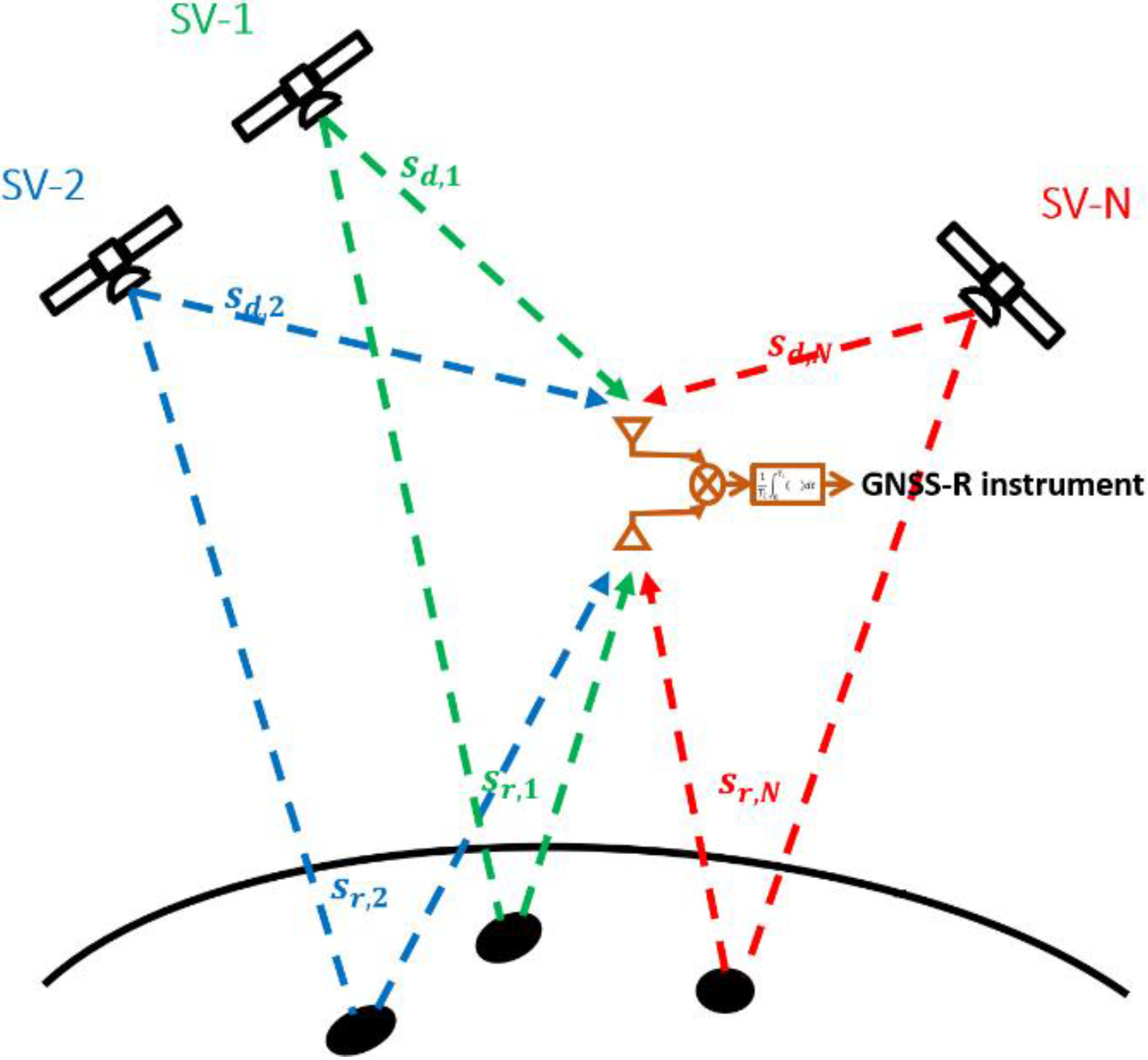
2. Methodology: EM Bias Estimation in Off-Nadir Configuration

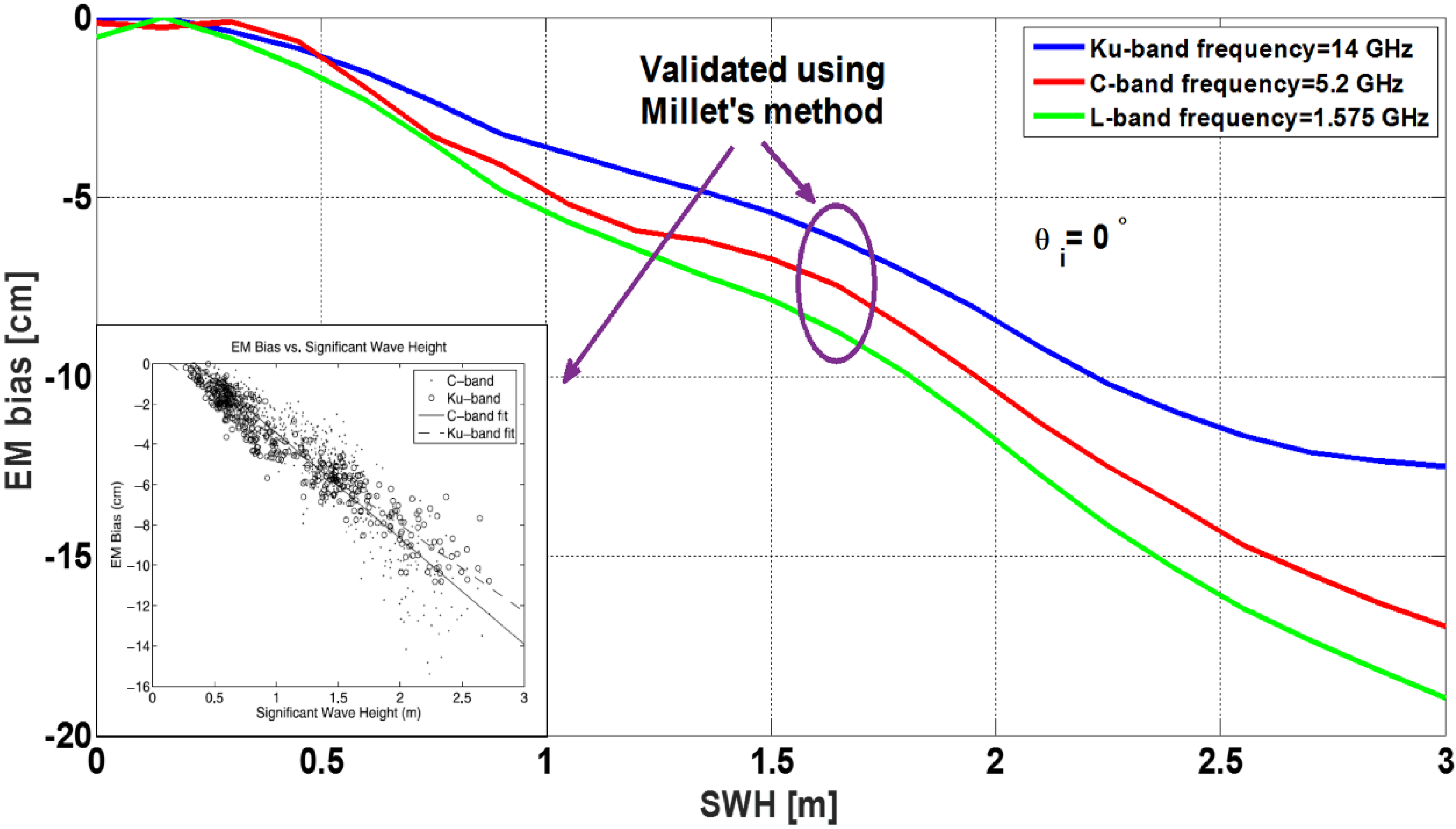
2.1. Implementation of Conventional Altimetry EM Bias Estimation Model at L-Band for GNSS-R

In conventional altimetry, the EM bias has been studied using the PO method at C- and Ku- bands [13]. This method proposed an analytical formula to estimate the EM bias. An analytical formulation demonstrated the relationship between the incidence angle and the EM bias, which was experimentally demonstrated in a few limited cases [13].

In this work, Millet’s et al. EM bias estimation method [13] is selected for validation purposes of the numerical method described in Section 2.2 because it allows to account for off-nadir conditions, as encountered in GNSS-R. The sea surface is generated using Elfouhaily’s spectrum [16], that can provide both short and long sea surface waves. This method [13] has been implemented, tested at C- (5.2 GHz) and Ku- (14 GHz) bands, and validated against experimental data (Figure 2). At this point, by selecting the appropriate cut-off wavenumber and using the corresponding dielectric constant it can be extrapolated at L-band (1.575 GHz). In our study, the well-known Klein and Swift model [18] is used, since in L-band reflectometry the impact of the dielectric constant is negligible (< 1%). Results are shown in Figure 2.

As shown in Figure 2, the EM bias increases with the significant wave height at C- (red) and Ku- (blue) bands, increasing (in absolute value) for lower frequency bands. The reference figure (Figure 8 from [13]) is overlaid with the obtained simulation results to show the goodness of the numerical method. Finally, the EM bias vs. significant wave height is estimated at L-band (green) using Millet’s et al. method. As it can be appreciated, the EM bias is much larger (in absolute value) than at other higher bands (C- and Ku-bands).

Figure 2. EM bias estimated using Millet’s et al. model, at C- (red) and Ku- (blue)-bands (Figure 8 from [13]), and extrapolated results at L-band (green) as a function of the Significant Wave Height (SWH). Modified from Figure 5 in [4].

Figure 2. EM bias estimated using Millet’s et al. model, at C- (red) and Ku- (blue)-bands (Figure 8 from [13]), and extrapolated results at L-band (green) as a function of the Significant Wave Height (SWH). Modified from Figure 5 in [4].

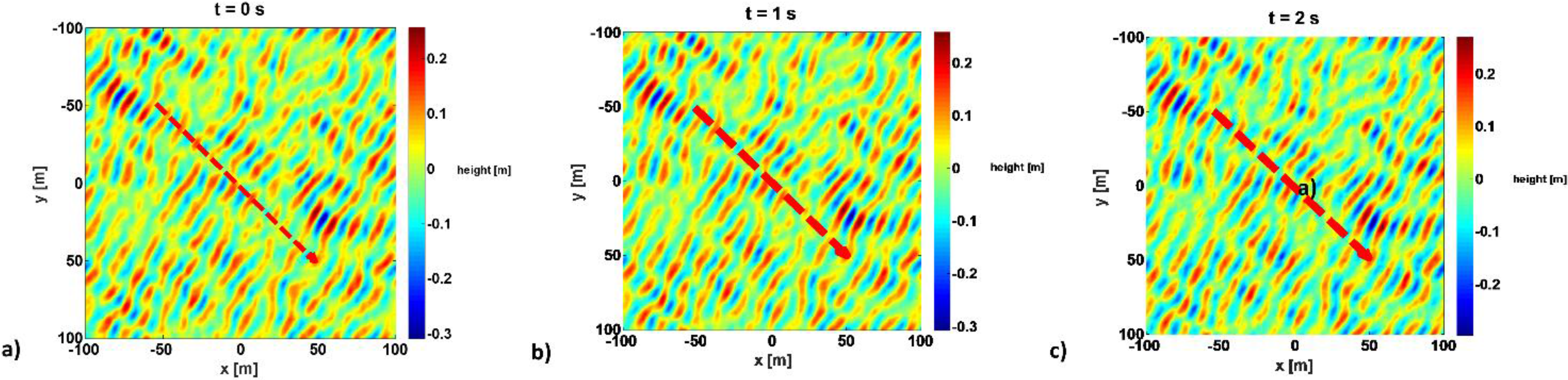
2.2. Numerical Computation of the EM Bias

The basic EM bias formulation is used as the ratio of the average of the radar cross-section density (σ⁰) times the sea surface elevation (ξ), and the average radar cross-section density [19]:

$${\text{β}}_{EM}=\frac{{\text{ξσ}}^0}{{\text{σ}}^0}.$$

(1)

Its interpretation is intuitive since wave valleys are flatter, provide a stronger return to the electromagnetic signal and appear brighter than the wave crests.

In order to estimate the time evolution of the EM bias, a time-domain simulator of the sea surface was designed and implemented. It includes four main blocks: the simulation of the transmitted Right Hand Circular Polarization (RHCP) electromagnetic wave (actually a multipath-free recorded GPS signal), the sea surface generator (using Elfouhaily’s directional spectrum), the generation of the scattered wave (using the KA-PO method), and the simulation of an antenna and receiver to collect the reflected waves and simulated the collected scattered fields, from where σ⁰ is estimated. The interested reader is referred to [4,15] for more details. In order to generate a reliable sea surface with wind-driven waves, and non-Gaussian height characteristics, an appropriate sea surface height spectrum has to be selected. In our study, the Elfouhaily’s directional sea surface height spectrum is used [16] to generate a 1000 m × 1000 m surface, so as to include the longest waves associated to the highest wind speed conditions simulated. Then, the incident wave illuminating the sea surface is created: a RHCP wave at L-band (f_L1 = 1.57542 GHz), which was actually pre-recorded using a GPS data-logger. The sea surface complex dielectric permittivity is set to ε_r = 73 + j·57.5. To meet the KA threshold, the average radius of the sea surface curvature must be larger than the electromagnetic wavelength [20]. The surface is then discretized in 20 cm × 20 cm patches. Then, the GPS wave scattered from the sea surface (mostly a left-hand circular polarization or LHCP) is computed using the PO scattering model under a bistatic configuration [21]. Finally, a uniformly illumination 5 × 5 patch antenna array with spacing of d_x = d_y = λ⁄2 is used to mimic the way the scattered waves are collected and weighted by the antenna pattern.

It should be mentioned that the synthesized sea surface has very large dimensions, as discussed in [4]. In this study, a 200 m × 200 m zoom of three consecutive snap-shots ξ(x,y,t) at t = 0–2 s are resented in Figure 3a–c. These snap-shots are captured under specific conditions: wind speed 2 m/s, wind direction φ = 45° (with respect to the y axis).

Figure 3. Three sea surface snap-shots for times (a) 0 s, (b) 1 s and (c) 2 s. Note that waves “propagate” and disperse while travelling along φ = 45° with respect to the y axis (looking direction). Colorbar indicates the sea surface height in meters.

Figure 3. Three sea surface snap-shots for times (a) 0 s, (b) 1 s and (c) 2 s. Note that waves “propagate” and disperse while travelling along φ = 45° with respect to the y axis (looking direction). Colorbar indicates the sea surface height in meters.

3. Results: Statistical Study of the Time-domain EM Bias

In this section, the EM bias is computed in the time-domain using the numerical method described above. The estimation of the EM bias in the time-domain requires the generation of the sea surface height in the time-domain explained above. Actually, the estimation of the EM bias as a function of time, even in steps of 1 s, significantly increases the computational cost. The variation of the instantaneous sea surface height ξ (x,y,t) impacts the scattering process, and therefore the radar cross-section density σ⁰ (x,y,t), the two variables from which the β_EM depends.

Later on, histograms of the time-domain EM bias will be computed and presented, as well as the first (mean), second (standard deviation), third (skewness), and fourth (kurtosis) moments. First, the time-domain evaluation and the dependence with the incidence and azimuth angles will be assessed.

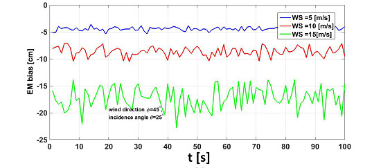
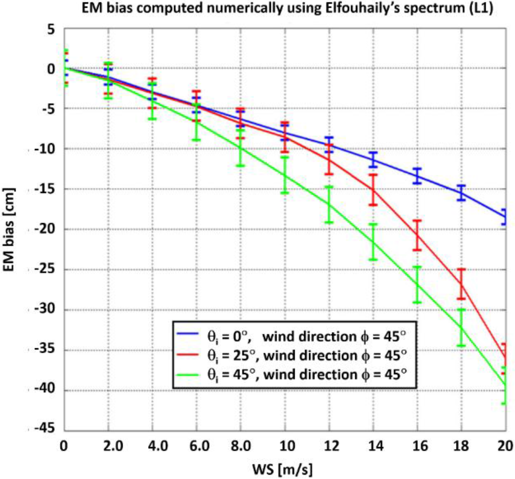
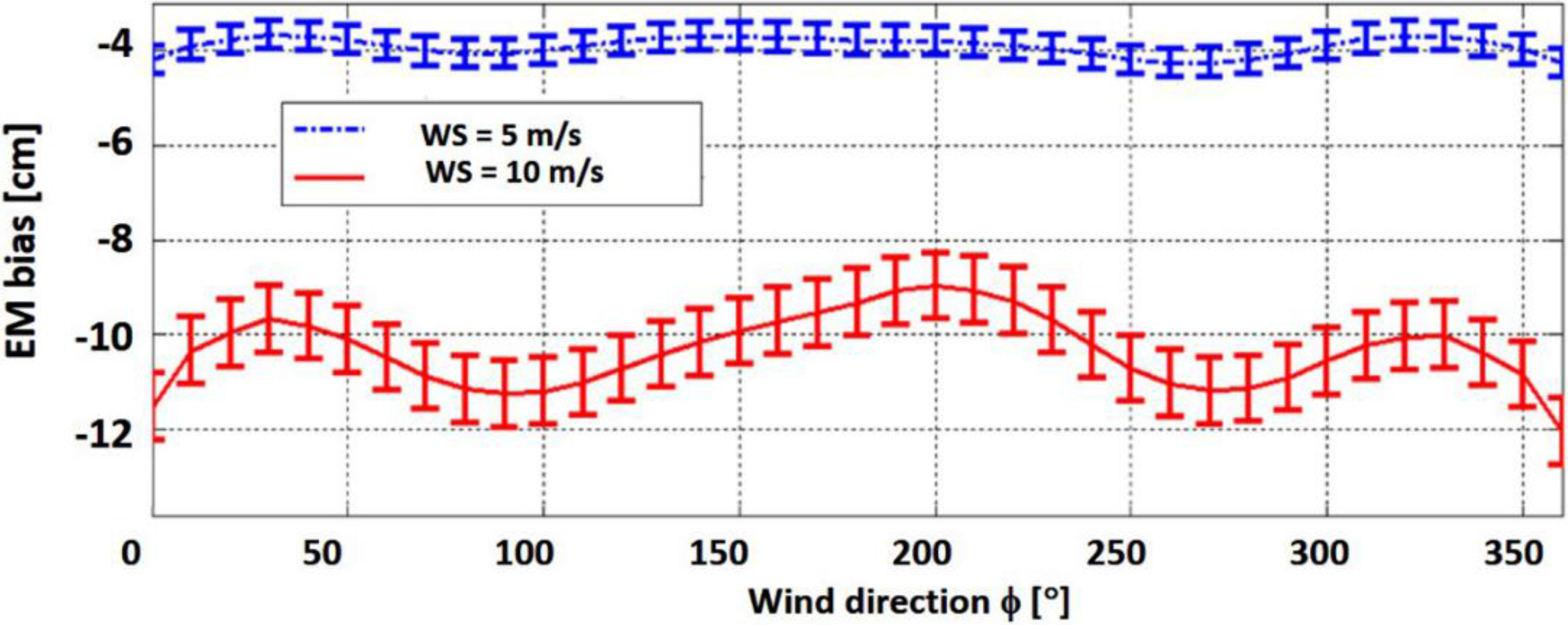
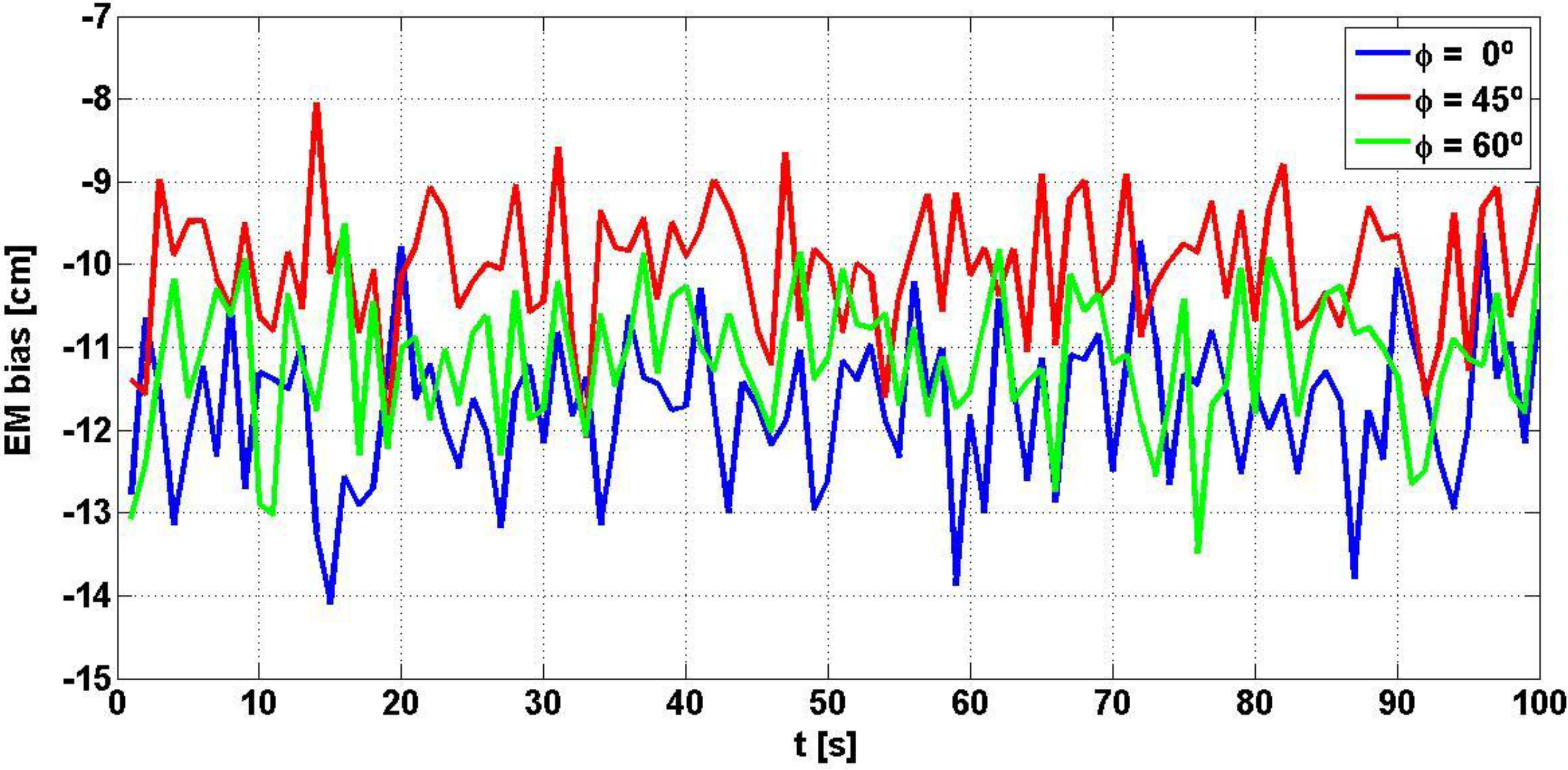
3.1. Computing Time-Domain EM Bias under Specific Incidence and Azimuth Angles

The estimated average EM bias is presented in Figure 4 for an incidence/scattering angle of 0° (nadir looking, monostatic case), 25°, and 45°, and a wind direction of 45° vs. the look direction, as a function of the wind speed. Other scenarios have been tested, including different time step (1 s), but results are indistinguishable. Error bars show the 95% confidence limits estimated from 10 Monte Carlo realizations. This numerical technique does not require many (e.g., > 10) Monte Carlo simulations because in each simulation many facets are already present and a large spatial averaging is already performed.

Figure 4. Estimated EM bias for θ_i = θ_s = 0°, 25°, and 45°and ϕ = 45°.

Figure 4. Estimated EM bias for θ_i = θ_s = 0°, 25°, and 45°and ϕ = 45°.

If the wind speed is set as a constant, but the sea waves evolve with time in time steps of 50 m/s, the time-domain evolution of the EM bias can be computed for each snap-shot. Results are presented in Figure 5 for θi = θs = 25°, and for three wind speeds: 5, 10, and 15 m/s. As it can be appreciated, increasing the wind speed not only increases (in absolute value) the average EM bias (β_EM), but its standard deviation ${\sigma }_{{\beta }_{EM}}$ as well (amplitude of the EM bias fluctuations). Quantitative results are discussed in Section 3.2.

Figure 5 shows another interesting feature, although the fluctuations of the EM bias are quite noisy, the higher the wind speed, the faster the fluctuations are due to the faster changes in the small scales, and not on the long waves, which actually travel at a much slower speed.

Figure 5. Computed time-evolution of the EM bias for wind speed WS = 5, 10, and 15 m/s, incidence/scattering angle θ_i = θ_s = 25°, and wind direction ϕ =45°.

Figure 5. Computed time-evolution of the EM bias for wind speed WS = 5, 10, and 15 m/s, incidence/scattering angle θ_i = θ_s = 25°, and wind direction ϕ =45°.

The EM bias was also computed in [4] as a function of the azimuth angle ϕ = 45°, for a constant incidence/scattering angle θ_i = θ_s = 25° for different wind speeds. Figure 6, shows the EM bias as a function of the azimuth angle. In fact, it exhibits an almost harmonic behavior that mimics that of the radar cross-section [22].

Next, the time-domain evaluation of the EM bias (over 100 s) is computed in 1s steps for three different wind directions φ = 0°, 45° and 60°, under an incidence/scattering angle of 25°, and a constant wind speed of 10 m/s. Results are shown in Figure 7. Despite the large fluctuation it is clear that the average value for ϕ = 45°, is larger than for ϕ = 0° and ϕ = 60°, as follows from the estimated values in Figure 6.

Figure 6. Impact of wind direction on EM bias from an incidence/scattering angle θ_I = θ_s = 25° and two different wind speeds (modified from [4]).

Figure 6. Impact of wind direction on EM bias from an incidence/scattering angle θ_I = θ_s = 25° and two different wind speeds (modified from [4]).

Figure 7. Time-domain evaluation of the EM bias for on incidence/scattering angle of 25° for three different wind directions 0°, 45° and 60°, during 100 s, in 1 s step.

Figure 7. Time-domain evaluation of the EM bias for on incidence/scattering angle of 25° for three different wind directions 0°, 45° and 60°, during 100 s, in 1 s step.

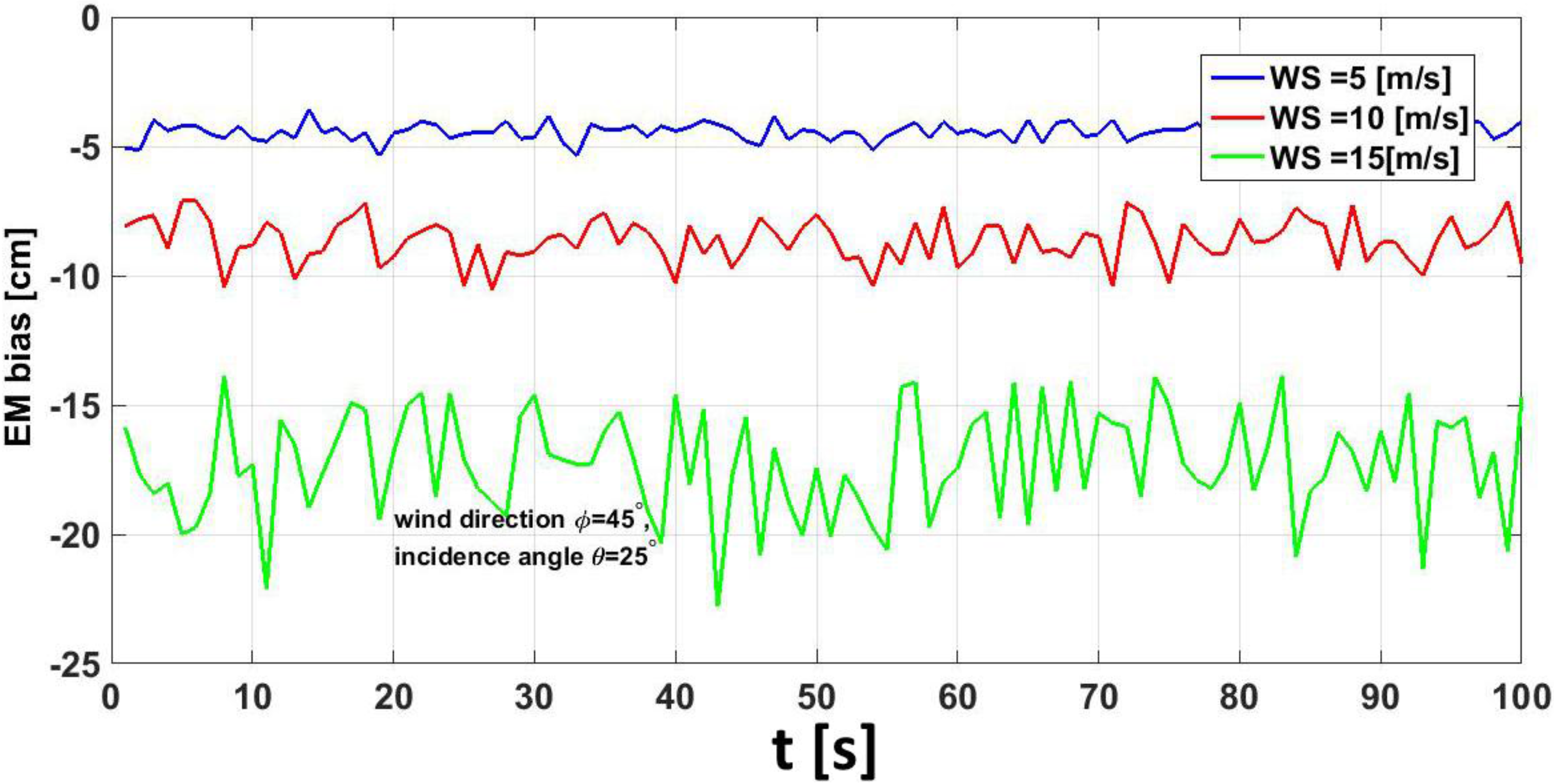
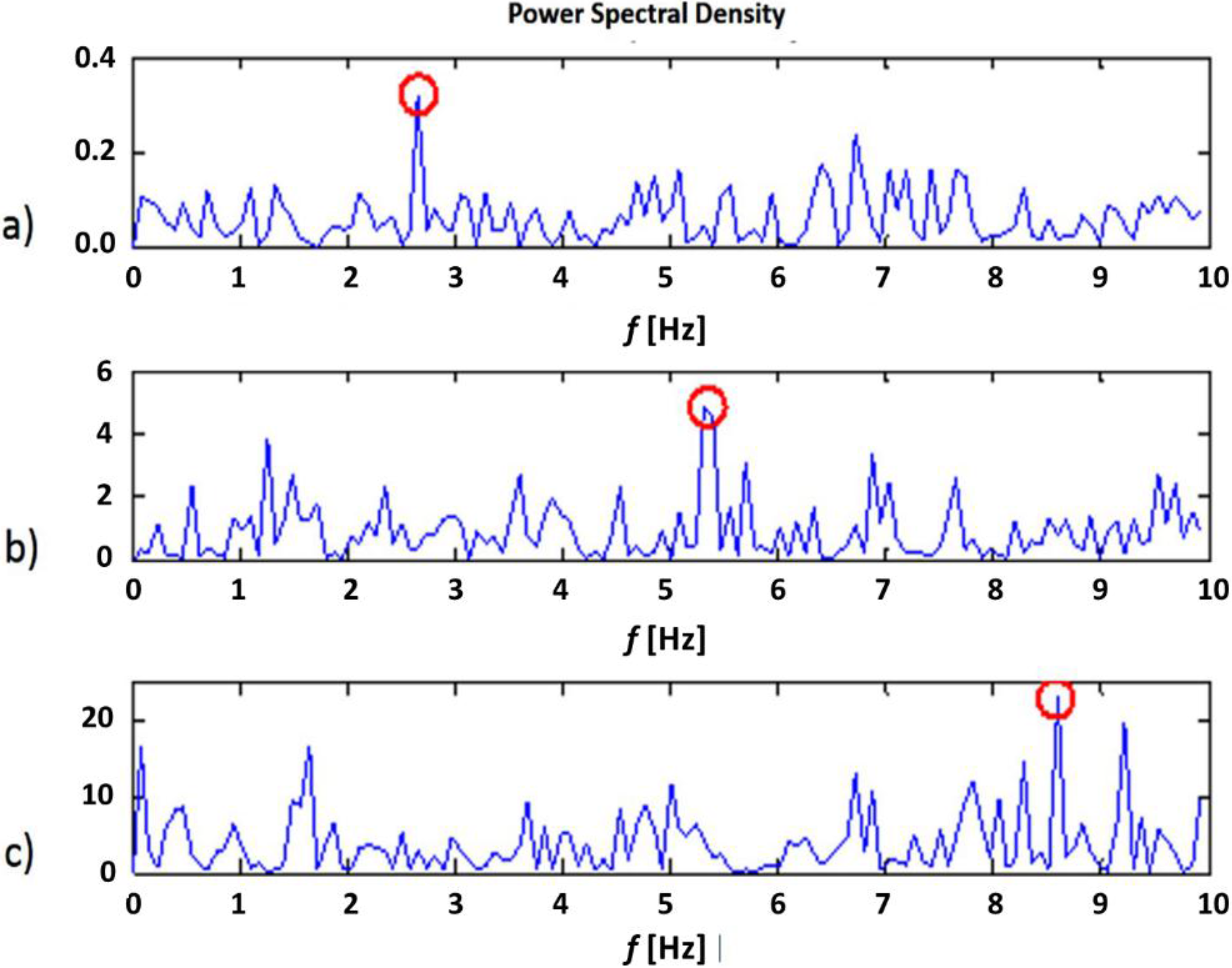
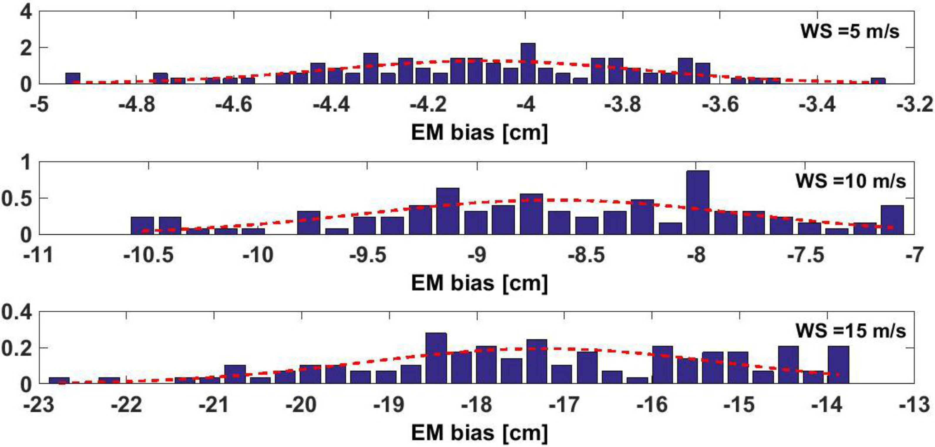
3.2. Non-Linearity Behavior of the Time-Domain EM Bias Descriptors

The estimated time-domain EM bias must inherit the dominant properties of the sea surface roughness and radar cross-section density, that is, it has to exhibit a Non-Gaussian behavior. In order to investigate this behavior, the time-domain EM bias power spectral densities and histograms are presented in Figure 8 and Figure 9.

Figure 8. Power spectral density of the EM bias fluctuation (mean removed) for incidence/scattering angle θ_i = θ_s = 25°, wind direction φ = 45°, and (a) U₁₀ = 5 m/s; (b) U₁₀ = 10 m/s; and (c) U₁₀ = 15 m/s.

Figure 8. Power spectral density of the EM bias fluctuation (mean removed) for incidence/scattering angle θ_i = θ_s = 25°, wind direction φ = 45°, and (a) U₁₀ = 5 m/s; (b) U₁₀ = 10 m/s; and (c) U₁₀ = 15 m/s.

Figure 9. Histograms of the EM bias time series for incidence/scattering θ_i = θ_s = 25°, wind direction φ = 45°, and (top) U₁₀ = 5 m/s; (center) U₁₀ = 10 m/s; (bottom) U₁₀ = 15 m/s.

Figure 9. Histograms of the EM bias time series for incidence/scattering θ_i = θ_s = 25°, wind direction φ = 45°, and (top) U₁₀ = 5 m/s; (center) U₁₀ = 10 m/s; (bottom) U₁₀ = 15 m/s.

Figure 8 shows that the EM peak frequency increases with increasing wind speed. Figure 9 shows the histograms of the EM bias time series for the three different wind speeds studied. Numerical results are shown in Table 1, Table 2 and Table 3. As it can be appreciated, for increasing wind speeds, the histograms become less Gaussian. The mean ${\overline{\beta }}_{EM}$ increases (in absolute value) with increasing wind speed, the standard deviation ${\sigma }_{{\beta }_{EM}}$ and the Skewness $S_{{\beta }_{EM}}$ increase as well, while the Kurtosis $K_{{\beta }_{EM}}$ slightly decreases. Table 1 shows that with increasing wind speeds, the EM bias histograms become more asymmetrical, with a more rounded peak around the mean (Kurtosis decreases), and depart from a Gaussian distribution [23].

Table 1. EM bias time series main statistical descriptors for incidence/scattering θ_i = θ_s = 0°, wind direction φ = 45°, and U₁₀ = 5 m/s, 10 m/s and 15 m/s.

U\10\ (m/s)	${\overline{\beta }}_{EM}$ (cm)	${\sigma }_{{\beta }_{EM}}$ (cm)	$S_{{\beta }_{EM}}$ (Unitless)	$K_{{\beta }_{EM}}$(Unitless)
5	−3.89	0.281	−0.451	5.31
10	−8.37	0.921	−0.490	5.01
15	−13.35	1.61	−0.598	4.35

Table 1. EM bias time series main statistical descriptors for incidence/scattering θ_i = θ_s = 0°, wind direction φ = 45°, and U₁₀ = 5 m/s, 10 m/s and 15 m/s.

U\10\ (m/s)	${\overline{\beta }}_{EM}$ (cm)	${\sigma }_{{\beta }_{EM}}$ (cm)	$S_{{\beta }_{EM}}$ (Unitless)	$K_{{\beta }_{EM}}$(Unitless)
5	−3.89	0.281	−0.451	5.31
10	−8.37	0.921	−0.490	5.01
15	−13.35	1.61	−0.598	4.35

Table 2. EM bias time series main statistical descriptors for incidence/scattering θ_i = θ_s = 25°, wind direction φ = 45°, and U₁₀ = 5 m/s, 10 m/s and 15 m/s.

U\10\ (m/s)	${\overline{\beta }}_{EM}$ (cm)	${\sigma }_{{\beta }_{EM}}$ (cm)	$S_{{\beta }_{EM}}$ (Unitless)	$K_{{\beta }_{EM}}$(Unitless)
5	−3.72	0.292	−0.475	5.44
10	−9.73	0.959	−0.493	5.03
15	−17.2	2.06	−0.592	4.84

Table 2. EM bias time series main statistical descriptors for incidence/scattering θ_i = θ_s = 25°, wind direction φ = 45°, and U₁₀ = 5 m/s, 10 m/s and 15 m/s.

U\10\ (m/s)	${\overline{\beta }}_{EM}$ (cm)	${\sigma }_{{\beta }_{EM}}$ (cm)	$S_{{\beta }_{EM}}$ (Unitless)	$K_{{\beta }_{EM}}$(Unitless)
5	−3.72	0.292	−0.475	5.44
10	−9.73	0.959	−0.493	5.03
15	−17.2	2.06	−0.592	4.84

Table 3. EM bias time series main statistical descriptors for incidence/scattering θ_i = θ_s = 45°, wind direction φ = 45°, and U₁₀ = 5 m/s, 10 m/s, and 15 m/s.

U\10\ (m/s)	${\overline{\beta }}_{EM}$ (cm)	${\sigma }_{{\beta }_{EM}}$ (cm)	$S_{{\beta }_{EM}}$ (Unitless)	$K_{{\beta }_{EM}}$(Unitless)
5	−4.96	0.176	−1.041	6.95
10	−13.8	0.691	−1.351	4.59
15	−24.1	1.28	−1.516	4.42

Table 3. EM bias time series main statistical descriptors for incidence/scattering θ_i = θ_s = 45°, wind direction φ = 45°, and U₁₀ = 5 m/s, 10 m/s, and 15 m/s.

U\10\ (m/s)	${\overline{\beta }}_{EM}$ (cm)	${\sigma }_{{\beta }_{EM}}$ (cm)	$S_{{\beta }_{EM}}$ (Unitless)	$K_{{\beta }_{EM}}$(Unitless)
5	−4.96	0.176	−1.041	6.95
10	−13.8	0.691	−1.351	4.59
15	−24.1	1.28	−1.516	4.42

4. Discussion

A GNSS-R instrument can be understood as a bistatic Synthetic Aperture Radar (SAR) using navigation signals as sources of opportunity with a very short integration time, as limited by the coherent integration time (typically T_i~1 ms), followed by long incoherent averaging so as to reduce speckle noise (typically N_incoh ranges from 1000 to 10000, corresponding to 1–10 s total integration) [24]. As for low-resolution SAR sensors (the case of GNSS-R instruments), the number of scatterers in the resolution cell is very large, 1Tthe statistics of SAR images follow the predictions of the Rayleigh model, and the Exponential model matches well the actual data (e.g., [25]). In this study, we have captured not only the time-average statistics of the scattered signal, and its impact on the EM bias, but its temporal dependence as well.

The EM bias is found not to exhibit a dependence only with the wind speed, the incidence/scattering angle, and the azimuth angle, but also a fluctuation with time, due to the temporal evolution of ξ(x,y,t) and those of σ⁰(x,y,t). For wind speeds from 5 to 15 m/s, the average bias changes from −4 to −13 cm at nadir, from −5 to −24 cm at θ_i = 45°, and the standard deviation changes from 0.3 cm to 2 cm.

By computing the time series of the EM bias under different wind speed conditions, it is found that not only the average value depends on the wind speed, but also the standard deviation, the Skewness, and Kurtosis. As the wind speed increases, the EM bias histograms depart from a Gaussian probability density function, and the standard deviation increases, which translates into a larger uncertainty of the EM bias itself. This is important, because noise should be reduced by incoherent averaging of the coherently integrated GNSS-R waveforms during the dwell time (typically, as long as dwell line / ground track speed = 100 km/6.5 km/s~15 s), and the EM bias should be cancelled from estimated values computed using auxiliary wind speed data (or more generically sea state data). However, since the EM bias does not follow a Gaussian distribution, EM bias fluctuations will not reduce as the square root of the number of incoherent averages.

5. Conclusions

In this work, the statistics of the time-domain evolution of the electromagnetic bias bias—one of the most challenging errors in altimetry—have been computed using a numerical simulator that allows: (1) to mimic the right hand circular polarization wave transmitted by navigation satellites, that impinges a synthetic time-evolving surface of the sea; (2) to compute the scattered fields using the Kirchoff Approxination-Physical Optics method; and (3) to numerically estimate the EM bias for each set of parameters (frequency, wind speed, incidence/scattering and azimuth angles…) using its fundamental definition, which removes a number of approximations or hypothesis made when dealing with analytic formulations. The electromagnetic bias fluctuations with time are found to exhibit a non-Gaussian probability density function, so it does not reduce as the square root of the number of measurements being averaged. The computed electromagnetic bias values and their dependence with geophysical and geometric parameters are important to predict the electromagnetic bias, so as to correct it in upcoming GNSS-R altimetry missions [25], such as the European Space Agency GEROS experiment on board the International Space Station [26,27], and to assess its impact in data assimilation studies, such as the one being performed in the “GNSS-Reflectometry Assessment of Requirements and Consolidation of Retrieval Algorithms” study in support of the GEROS experiment.

References

1. Hall, C.D.; Cordey, R.A. Multistatic scatterometry. In Proceedings of the 1988 IEEE International Geoscience Remote Sensing Symposium, Seattle, WA, USA, 6–10 July 1998; pp. 561–562.
2. Martin-Neira, M.A. Passive reflectometry and interferometry system (PARIS): Application to ocean altimetry. ESA J. 1993, 17, 331–355. [Google Scholar]
3. Radar Altimetry Tutorial. Available online: http://www.altimetry.info/ (accessed on 10 August 2015).
4. Ghavidel, A.; Schiavulli, D.; Camps, A. Numerical computation of the electromagnetic bias in GNSS-R altimetry. IEEE T Geosci Remote Sens. 2015. [Google Scholar] [CrossRef]
5. Yaplee, B.S.; Shapiro, A.; Hammond, D.L.; Au, B.D.; Uliana, E.A. Nanosecond radar observations of the ocean surface from a stable platform. IEEE T. Geosci. Electron. 1971, 9, 170–174. [Google Scholar] [CrossRef]
6. Jackson, F.C. The reflection of impulses from a nonlinear random sea. J. Geophys. Res. Ocean. 1979, 84, 4939–4943. [Google Scholar] [CrossRef]
7. Srokosz, M.A. On the joint distribution of surface elevation and slopes for a nonlinear random sea, with an application to radar altimetry. J. Geophys. Res. Ocean. 1986, 91, 995–1006. [Google Scholar] [CrossRef]
8. Glazman, R.E.; Fabrikant, A.; Srokosz, M.A. Numerical analysis of the sea state bias for satellite altimetry. J. Geophys. Res. Ocean. 1996, 101, 3789–3799. [Google Scholar] [CrossRef]
9. Elfouhaily, T.; Thompson, D.; Vandemark, D.; Chapron, B. Weakly nonlinear theory and sea state bias estimations. J. Geophys. Res. Ocean. 1999, 104, 7641–7647. [Google Scholar] [CrossRef]
10. Elfouhaily, T.; Thompson, D.R.; Vandemark, D.; Chapron, B. Higher-order hydrodynamic modulation: theory and applications for ocean waves. Proc. R. Soc. Lond. A 2001, 457, 2585–2608. [Google Scholar] [CrossRef]
11. Walsh, E.J.; Jackson, F.C.; Hines, D.E.; Piazza, C.; Hevizi, L.G.; Mclaughlin, D.J.; Mcintosh, R.E.; Swift, R.N.; Scott, J.F.; Yungel, J.K.; et al. Frequency dependence of electromagnetic bias in radar altimeter sea surface range measurements. J. Geophys. Res. Ocean. 1991, 96, 20571–20583. [Google Scholar] [CrossRef]
12. Hevizi, L.G.; Walsh, E.J.; McIntosh, R.E.; Vandemark, D.; Hines, D.E.; Swift, R.N.; Scott, J.F. Electromagnetic bias in sea surface range measurements at frequencies of the TOPEX/POSEIDON satellite. IEEE T. Geosci. Remote Sens. 1993, 31, 376–388. [Google Scholar] [CrossRef]
13. Millet, F.W.; Warnick, K.F.; Arnold, D.V. Electromagnetic bias at off-nadir incidence angles. J. Geophys. Res. Ocean. 2005, 110, 1–13. [Google Scholar] [CrossRef]
14. Millet, F.W.; Warnick, K.F.; Nagel, J.R.; Arnold, D.V. Physical optics-based electromagnetic bias theory with surface height-slope cross-correlation and hydrodynamic modulation. IEEE T. Geosci. Remote Sens. 2006, 44, 1470–1483. [Google Scholar] [CrossRef]
15. Ghavidel, A.; Schiavulli, D.; Camps, A. A numerical simulator to evaluate the electromagnetic bias in GNSS-R altimetry. In Proceedings of the 2014 IEEE International Geoscience and Remote Sensing Symposium, IGARSS 2014, Quebec, QC, Canada, 13–18 July 2014; pp. 4066–4069.
16. Elfouhaily, T.; Chapron, B.; Katsaros, K.; Vandemark, D. A unified directional spectrum for long and short wind-driven waves. J. Geophys. Res. Ocean. 1997, 102, 15781–15796. [Google Scholar] [CrossRef]
17. Tatarskii, V.I.; Tatarskii, V.V. Statistical non-Gaussian model of sea surface with anisotropic spectrum for wave scattering theory. Part II. Prog. Electromagn. Res. 1999, 22, 259–291. [Google Scholar] [CrossRef]
18. Klein, L.A.; Swift, C.T. An improved model for the dielectric constant of sea water at microwave frequencies. IEEE Trans. Antennas Propag. 1977, 25, 104–111. [Google Scholar] [CrossRef]
19. Elfouhaily, T.; Thompson, D.R.; Chapron, B.; Vandemark, D. Improved electromagnetic bias theory. J. Geophys. Res. Ocean. 2000, 105, 1299–1310. [Google Scholar] [CrossRef]
20. Clarizia, M.P.; Gommenginger, C.; Bisceglie, M.D.; Galdi, C.; Srokosz, M.A. Simulation of L-band bistatic returns from the ocean surface: A facet approach with application to ocean GNSS reflectometry. IEEE T. Geosci. Remote Sens. 2012, 50, 960–971. [Google Scholar] [CrossRef]
21. Zavorotny, V.U.; Voronovich, A.G. Scattering of GPS signals from the ocean with wind remote sensing application. IEEE T. Geosci. Remote Sens. 2000, 38, 951–964. [Google Scholar] [CrossRef]
22. Ulaby, F.T.; Moore, R.K.; Fung, A.K. From theory to applications. In Microwave Remote Sensing: Active and Passive; Artech House: Norwood, MA, USA, 1986; Volume 3, p. 1120. [Google Scholar]
23. Brown, S. Measures of Shape: Skewness and Kurtosis. Available online: http://brownmath.com/stat/shape.htm (accessed on 3 July 2015).
24. Valencia, E.; Camps, A.; Marchan-Hernandez, J.F.; Park, H.; Bosch-Lluis, X.; Rodriguez-Alvarez, N.; Ramos-Perez, I. Ocean surface’s scattering coefficient retrieval by Delay-Doppler Map inversion. IEEE Geosci. Remote Sens. Lett. 2011, 8, 750–754. [Google Scholar] [CrossRef]
25. Di Martino, G.; Iodice, A.; Riccio, D.; Ruello, G. A physical approach for SAR speckle simulation: First results. Eur. J. Remote Sens. 2013, 46, 823–836. [Google Scholar] [CrossRef]
26. Camps, A.; Park, H.; Valencia i Domenech, E.; Pascual, D.; Martin, F.; Rius, A.; Ribo, S.; Benito, J.; Andres-Beivide, A.; Saameno, P.; et al. Optimization and performance analysis of interferometric GNSS-R altimeters: Application to the PARIS IoD mission. IEEE J. Sel. Topics Appl. Earth Observ. Remote Sens. 2014, 7, 1436–1451. [Google Scholar] [CrossRef]
27. Mapping Sea Surface from the Space Station. http://www.esa.int/Our_Activities/Observing_the_Earth/Mapping_sea_surface_from_the_Space_Station (accessed on 3 July 2015).