Pairwise-Distance-Analysis-Driven Dimensionality Reduction Model with Double Mappings for Hyperspectral Image Visualization

Abstract

This paper describes a novel strategy for the visualization of hyperspectral imagery based on the analysis of image pixel pairwise distances. The goal of this approach is to generate a final color image with excellent interpretability and high contrast at the cost of distorting a few pairwise distances. Specifically, the principle of equal variance is introduced to divide all hyperspectral bands into three subgroups and to ensure the energy is distributed uniformly between them, as in natural color images. Then, after detecting both normal and outlier pixels, these three subgroups are mapped into three color components of the output visualization using two different mapping (i.e., dimensionality reduction) schemes for the two types of pixels. The widely-used multidimensional scaling (MDS) is used for normal pixels and a new objective function, taking into account the weighting of pairwise distances, is presented for the outlier pixels. The pairwise distance weighting is designed such that small pairwise distances between the outliers and their respective neighbors are emphasized and large deviations are suppressed. This produces an image with high contrast and good interpretability while retaining the detailed information content. The proposed algorithm is compared with several state-of-the-art visualization techniques and evaluated on the well-known AVIRIS hyperspectral images. The effectiveness of the proposed strategy is substantiated both visually and quantitatively.

1. Introduction

Hyperspectral remote sensors can collect data simultaneously in hundreds of narrow, adjacent spectral bands covering the visible to near-infrared wavelengths. The resulting hyperspectral images contain a wealth of high-resolution spectral information permitting a wide range of remote sensing applications, such as environment monitoring, geological surveying, and surveillance. However, visualizing the information content of this high-dimensional data space is difficult and often involves trade-offs between the complexity of information being conveyed, similarity of the output to the human visual system, and speed of visualization display.

Hyperspectral image visualization has been part of remote sensing for decades in order to provide a quick overview and understanding of a hyperspectral data set. Visualization is implemented by mapping the original high-dimensional data into a three-dimensional color space and showing the mapped data on a tristimulus-based display device (e.g., a standard computer screen). There is inevitable loss of information in the process of visualization. However, in order to effectively preserve the information contained in hyperspectral imagery and to intuitively provide a discriminative color representation, some objective visualization criteria have been proposed, including pairwise distance preservation [1–3] and feature separability (or contrast) [4,5]. The former tries to maintain pairwise distances in hyperspectral imagery and in the final color image while the latter, introduced by Cui et al. [4], aims to display the differences between pixels as distinctively as possible. It is difficult to simultaneously satisfy these two criteria since the smaller differences between pixels cannot be well distinguished when all pairwise distances are exactly preserved in the final color image. From the subjective perspective, the visualization aim is to generate a trichromatic composite image with perceptual appeal [6–8] suitable for interpretation by the human visual system, referred to as naturalness. However, it is challenging to display the full information content in mapped data on devices designed for natural images.

In the literature, many visualization methods have been proposed for hyperspectral images and can be roughly classified into four categories: band selection, linear spectral combination, data projection, and convex optimization.

Band selection refers to techniques that select three representative bands as color components. The simplest scheme is to pick three bands with wavelengths closest to the natural wavelengths of red, green and blue. More sophisticated rule based approaches, such as one-bit transform (1BT) [9], normalized information (NI) [6], minimum redundancy maximum relevance (mRMR) [10], minimum estimated abundance covariance (MEAC) and linear prediction [11], have also been introduced for the selection of triplet bands. However, this kind of techniques usually loses a large amount of information contained in the data space not represented in the three bands.

Another kind of visualization method is linear spectral combination. The idea is to create the final image from a weighted sum of pixels across the available sampled wavelength spectrum. The design of the weights involved is typically related to the visualization effect. In [3], a set of fixed spectral weighting envelopes are derived from color matching functions, designed to mimic how human photopic (daylight) vision works. In [12], a bilateral filtering scheme is presented for retaining the minor details, while, more recently, a multiobjective optimization-based approach has been proposed to provide the solution of weights by taking some desired properties of the resultant image into account [7]. Relatively speaking, the fused images are more informative due to the process of combining information from all bands.

The third family of visualization methods is composed of data transformations that aim to project the original hyperspectral image into a low-dimensional space. The classical example is principal component analysis (PCA), which has been extensively used for visualization purposes. In general, PCA and its variants are explored as an N-to-3 projection into the color space with the first three principal components [13–15]. Further PCA methods have been investigated based on perceptual attributes [16] and class separability [17]. An alternative way, i.e., segmented PCA, is to perform PCA on three subgroups to extract principal components used for visualization [18,19]. Additionally, regarding the nonlinear characteristics of hyperspectral data [20], a straightforward but time-consuming extension is to employ nonlinear projection methods (e.g., local linear embedding) for dimensionality reduction into three bands with the goal of preserving the local distances between a pixel and its neighbors.

A new class of visualization methods, designed to preserve some desired properties, was recently proposed from the convex optimization perspective by formulating the related criteria into the underlying objective function. In [4], Cui et al. exploited pairwise distance preservation and feature separability in a two-step dimensionality-reduction framework. In their approach, the pairwise distance preservation criterion is explicitly set as a three-dimensional mapping problem decomposed into two steps: a two-dimensional projection as a partial solution using classical PCA and a linear programming method to solve for the one-dimensional coordinate in the third dimension with the separability of features criterion as a set of constraints. From a different perspective, Mignotte proposed a bicriteria optimization for color display model (BCOCDM) method [5] by combing these two contradictory criteria with an internal parameter, thus making this algorithm express the contribution of two criteria for a specific application, besides only focusing on the criterion of pairwise distance preservation in [21]. This kind of visualization method provides interesting and promising results to some extent.

These existing algorithms either favor distances preservation in high-dimensional space at the risk of low contrast or prefer high contrast for achieving the good features separability in the low-dimensional space but allow excessive distortion of the pairwise-distances or sometimes unwanted loss of the local details. More importantly, the intrinsic properties of the pairwise measured space for high-dimensional hyperspectral data, such as large-scale dynamic range of pairwise distances and concentration phenomenon, make it difficult for them to yield a natural visual representation.

In this paper, we propose a new hyperspectral image visualization strategy with double mappings for improved balancing of the trade-off between pairwise distance preservation and feature separability. Our contributions are three-fold:

• In order to decrease the dynamic range of pairwise distances and uniformly distribute energy in the three color components as that in natural color images, the principle of equal variance is adapted to divide the hyperspectral image bands into three subgroups prior to further mapping.
• Two different mapping methods are proposed for normal pixels and outlier pixels respectively. This can achieve good contrast with minimal distortion of the pairwise distances while preserving local fine information.
• In the mapping case of outlier pixels, an objective function, based on the weighting of pairwise distances, is designed to adaptively inhibit/enhance the large/small pairwise-distances for the purpose of preserving local topology in the hyperspectral data space.

The reminder of this paper is organized as follows. Section 2 analyzes the characteristics of pairwise distances in hyperspectral imagery and discusses the display problems of color space mapped data. Section 3 describes the pairwise-distances-analysis-driven visualization strategy (PDADVS) with double mappings. Experimental results and comparisons with existing methods are presented in Section 4, followed by concluding remarks in Section 6.

2. Problem Statement

Despite the progress of visualization methods, intrinsic measure phenomena of the high-dimensional hyperspectral data space are often overlooked. As such, this section presents important characteristics of pairwise distances in hyperspectral images and highlights how these properties may affect the visualization performance.

2.1. Analysis of Pairwise Distances in Hyperspectral Images

Visualization of hyperspectral imagery attempts to reduce the data dimensionality while retaining the information content of the full data space. Toward this goal, pairwise distance preservation is a good foundation for hyperspectral visualization because keeping pairwise distances in the visualized data space indicates a good mapping with high faithfulness of a resultant color image to raw hyperspectral data.

Before proceeding to the analysis of pairwise distances, we first define the notations used in what follows. Let I be a hyperspectral image of w × h pixels with r bands in a tensor space T_r ∈ ℝ^w×h×r, and $I_m^{1\sim r}$ be spectral vector (also is corresponding to a hyperspectral image pixel) with the subscript denoting the spatial location and the superscript denoting the range of bands. A subgroup of hyperspectral image is referred to as I^k1~k2, whose spectral vector is $I_m^{k1\sim k2}$. The pairwise distance $d_{m,n}^{I^{k1\sim k2}}$ between two spectral vectors $I_m^{k1\sim k2}$ and $I_n^{k1\sim k2}$ is defined as $d_{m,n}^{I^{k1\sim k2}}=\sqrt{\parallel I_m^{k1\sim k2}-I_n^{k1\sim k2}{\parallel }_2^2}$, which can be straightforwardly extended to the full-band case with k1 = 1 and k2 = r.

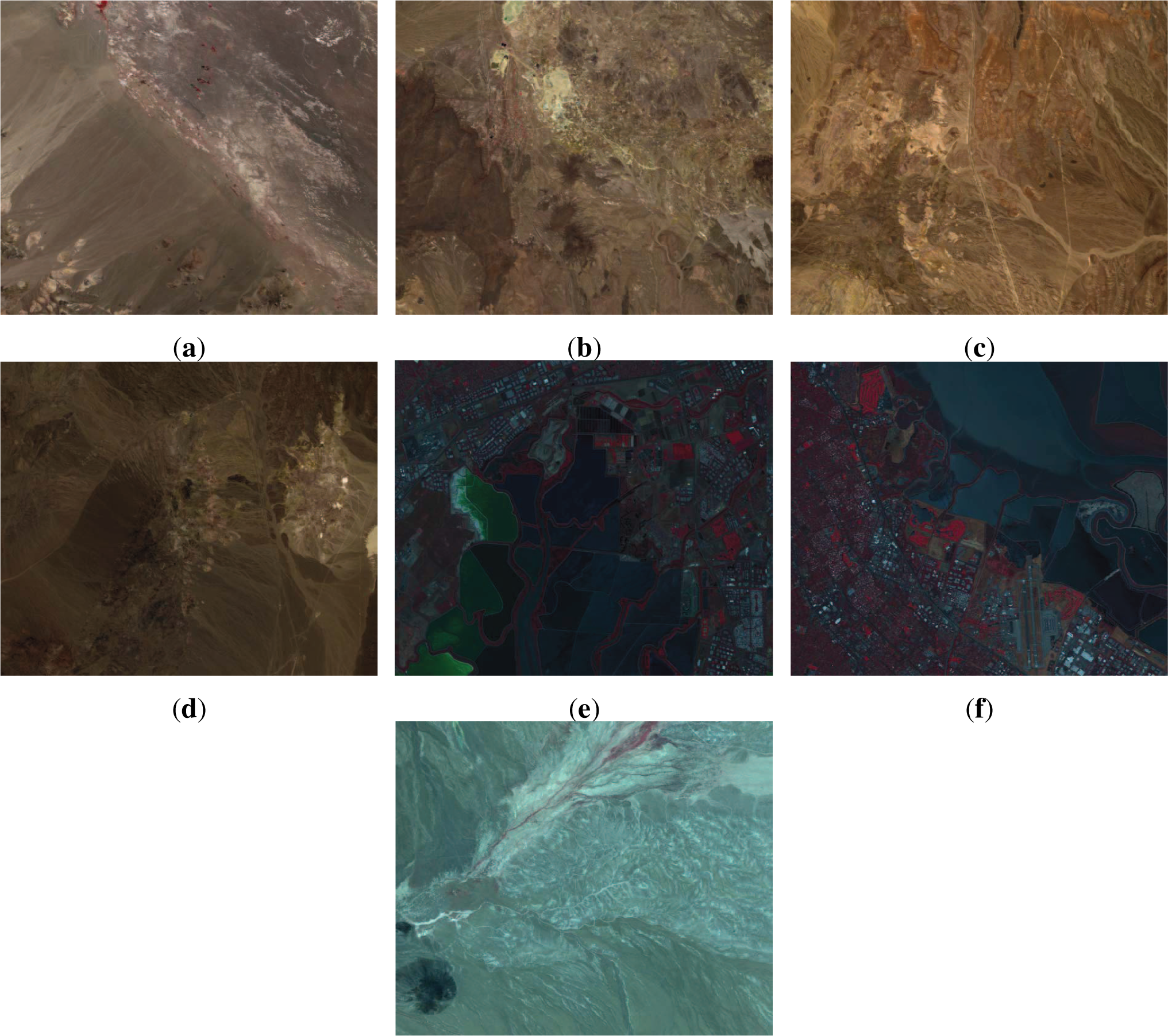
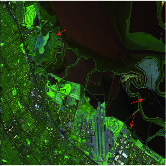
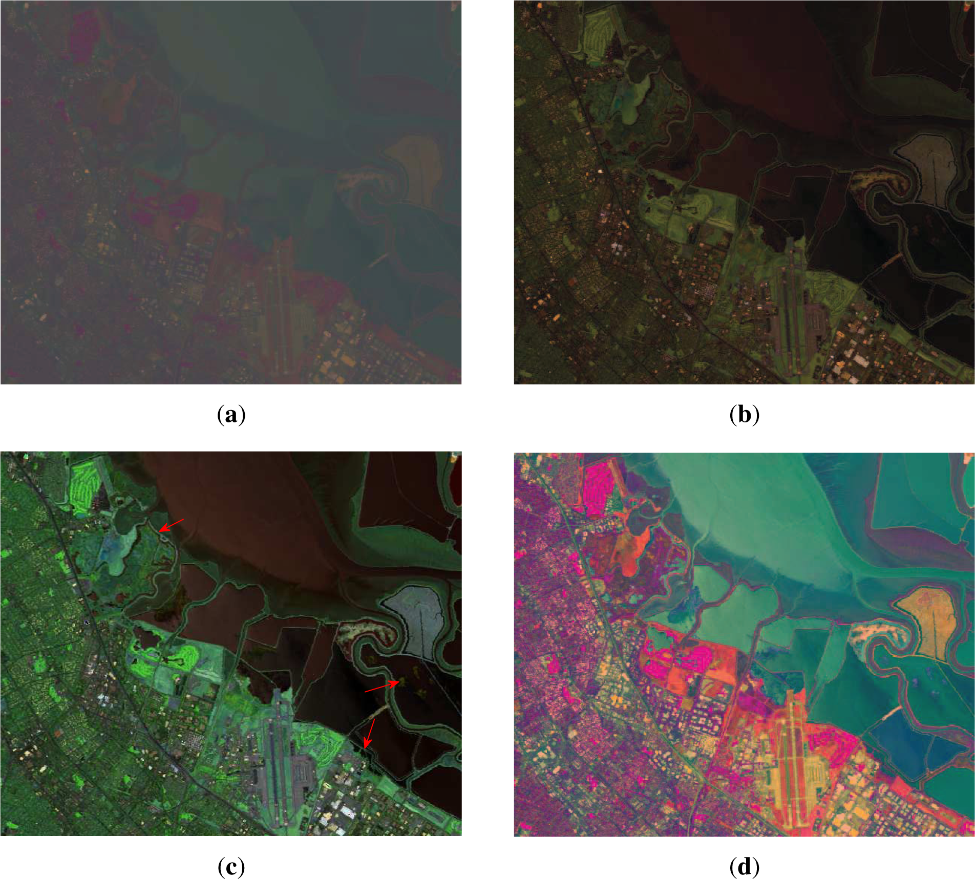
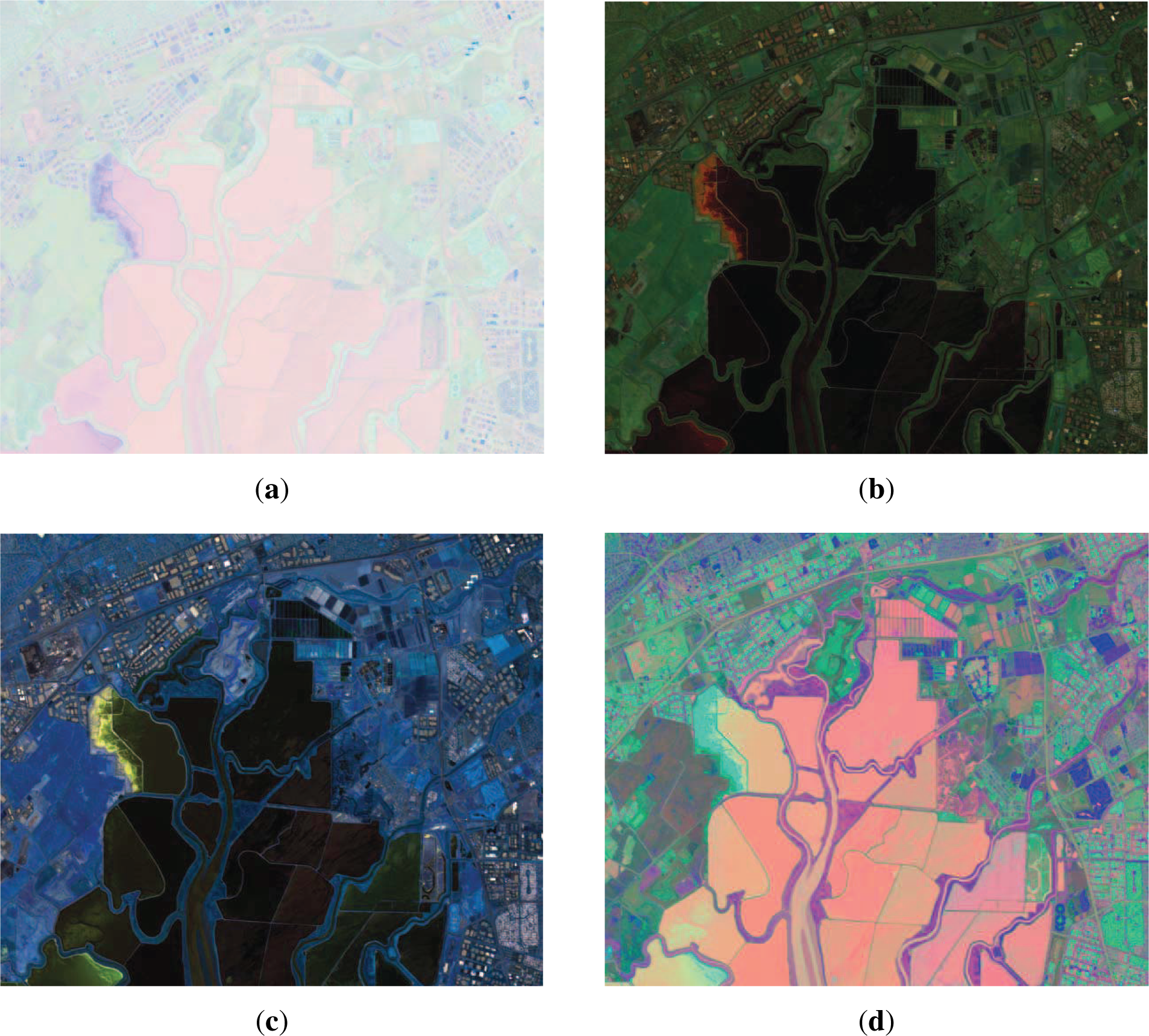
The images used later for experimental validation are taken as examples to illustrate the characteristics of pairwise distances in hyperspectral images, whose false-color composites are presented in Figure 1. In all cases, the black and noise bands are first removed as outlined in Section 3.2.

Table 1. Variances and ranges of pairwise distances for different subgroups of seven hyperspectral images.

Subgroups	Lun.lake01	Cuprite02	Cuprite03	Cuprite04	Moffet02_igm	Moffet03_igm	Lun.lake_igm
1 ∼ 60	24.3(254)	41.4(364)	32.8(295)	28.9(414)	24.3(254)	18.8(226)	44.4(400)
61 ∼ 120	37.7(298)	56.0(485)	40.5(380)	35.9(452)	27.7(298)	12.6(96)	20.5(191)
121 ∼ 190	28.0(327)	52.3(460)	44.6(443)	28.9(436)	28.0(327)	8.7(99)	15.9(153)
1 ∼ 100	32.0(326)	58.8(510)	45.3(431)	41.9(562)	32.0(326)	21.4(240)	47.8(437)
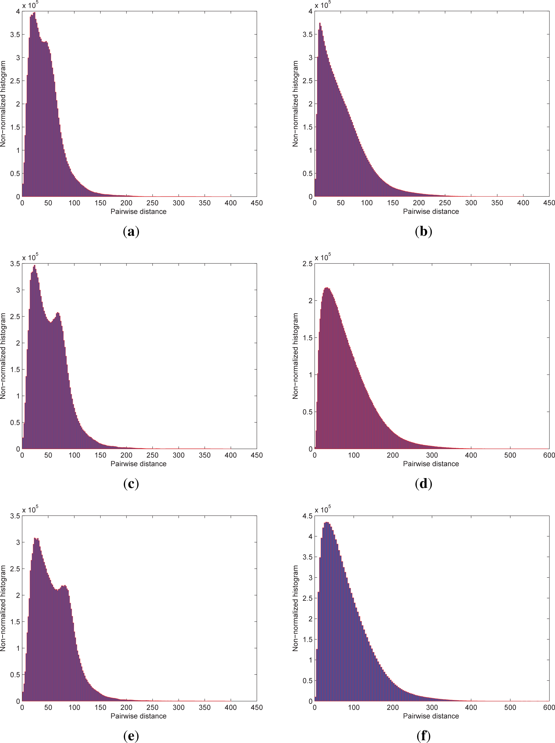
all bands	44.0(503)	82.6(739)	63.7(647)	51.7(761)	44.0(503)	22.8(246)	56.8(470)

lists the measures of pairwise-distance variation for different subgroups of seven hyperspectral images, while Figure 2 shows the non-normalized histograms of pairwise distances of Moffet₀₂_igm and Cuprite₀₂ with different band coverage for the intuitive analysis.

As shown in Table 1 and Figure 2, pairwise distances are distributed in a very wide range and exhibit heavy-tailed characteristics. In addition, the distributions show both increased variance and dynamic range as the dimensionality of the subgroups increase. Figure 2 reveals that the majority of pairwise distances populate the smaller distance values, which is consistent with the phenomenon of measure concentration in high-dimensional space [22–24]. Furthermore, the average and maximum quantities of pairwise distances together with their ratios are presented in

Table 2. Average and maximum quantities of pairwise distances for all of the available bands.

Subgroups	Lun.lake01	Cuprite02	Cuprite03	Cuprite04	Moffet02_igm	Moffet03_igm	Lun.lake_igm
mean	68.4	126.0	106.8	73.2	68.4	22.8	56.8
max	506	743	654	765	506	246	470
max/mean	8.7	5.9	6.1	10.5	7.4	10.8	8.3

for all available bands of seven hyperspectral images. In general, the mean is significantly less than the corresponding maximum value for each image. As a result, the dissimilarities represented by smaller pairwise distances become less meaningful because of their poor discernibility. On the contrary, a few larger pairwise distances indicate that some pixels are considerably dissimilar from the normal ones and are considered outliers as in [4,25,26], whose ranking and detection will be discussed in Section 3.3.

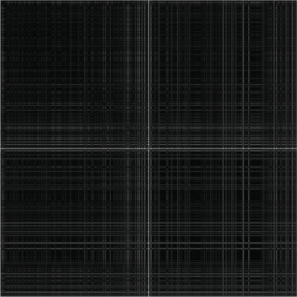
In order to further demonstrate the inconsistency of outlier pixels, the normalized pairwise-distance matrix image of an outlier located in (183, 211) and 512 randomly selected normal pixels extracted from Cuprite₀₂ image is shown in Figure 3. To construct this matrix, the outlier pixel is positioned in the median x-/y-coordinates. In this illustration, with white points denoting the high degree of dissimilarity, it is clear that large distances between this outlier and the normal pixels are much larger than that calculated among the normal pixels. Large pairwise distances is another consequence of the existence of outlier pixels, besides high dimensionality of hyperspectral images. Therefore, careful handling is necessary for the optimal visualization of hyperspectral data.

2.2. Display Problems of The Mapped Data in Color Space

To visualize hyperspectral images, the mapped data will be displayed on a standard tristimulus device, whose gamut is restricted to a triangle in chromaticity space and three primary colors generally have fixed quantization levels. Under the criterion of pairwise distance preservation, the characteristics of pairwise distances in the color space are similar to that of pairwise distances in the original high-dimensional space. Then the dynamic range, as that in the original high-dimensional space, will become large accordingly with the increase of dimensionality. Naturally, each color value will represent a larger pairwise-distance range. In addition, due to the concentration of measure phenomenon, the quantizing levels in each component of three primaries, associated with the majority of normal pixels, only account for a small central part {a + 1, a + 2,…, b − 1} of the whole gray level set G = {0, 1, 2,…, L}, while the top and bottom parts of this set, i.e., {0, 1, 2,…, a} and {b, b + 1,…, L}, are used to indicate a small number of the outlier pixels. As a result, the differences between normal pixels, represented by small pairwise distances, are difficult to distinguish in the color image and has poor contrast. Meanwhile, like the outliers originally measured in the high-dimensional space, their counterparts in the color space are few and far way from other color pixels. This makes it difficult to illustrate the pixel diversity in the mapped color space.

These difficulties have been explored by previous research and many techniques have been proposed to achieve a preferable visual effect. In this simplest case, these pixels, whose duplicates in the color image are so large that they suppress the brightness of other pixels, can be removed before dimensionality reduction [27]. In [3], Jacobson et al. proposed to render no more than 2% of pixels by clipping their out-of-gamut color values to the gamut in sRGB after fixed integration envelopes are applied. PCA2% used in ENVI linearly stretches each of three display bands so that 2% of pixels at both ends of each color channel are at the minimum and maximum display value. 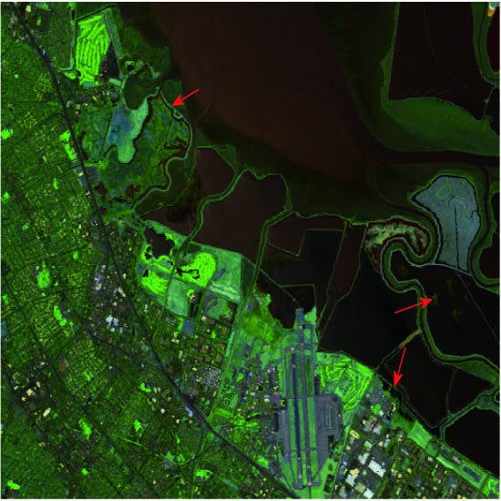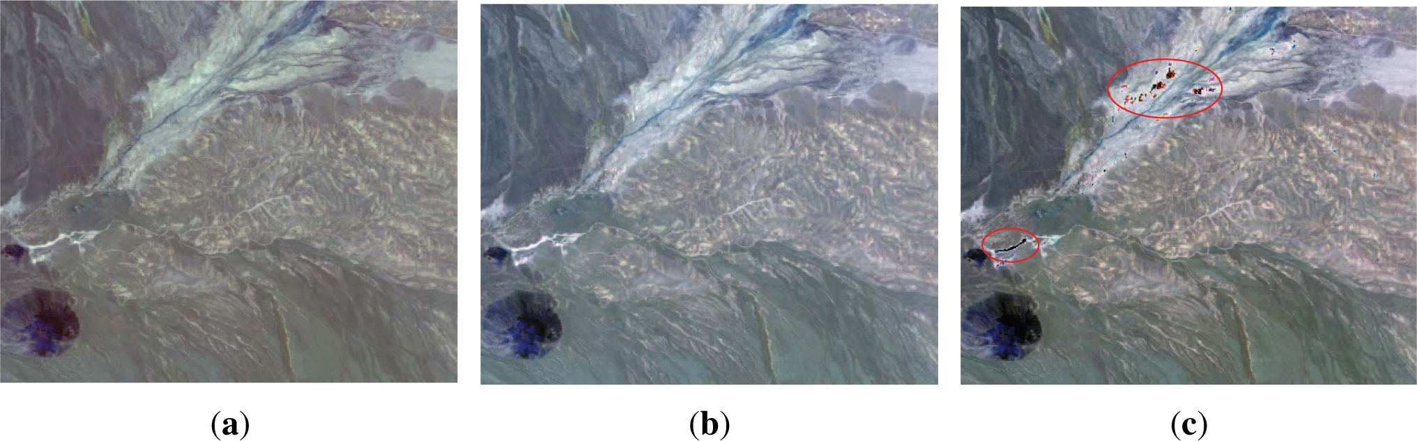However, in these cases, some pixels (i.e., outliers) regarded as a nuisance which impede the contrast enhancement tend to be eliminated. Although this creates a vivid contrast in some regions, the dissimilarities between outliers, which contain useful information, are lost. Furthermore, the local contrast where these outliers exist cannot be reflected in the visualized color image even though they have topological structure in a local region as shown in Figure 4. Good visualization cannot be achieved unless the visualization method is designed specifically to take these outliers, as well as the more general properties of hyperspectral images, into account. This is the motivation of our proposed method described in next section.

3. Proposed Visualization Technique

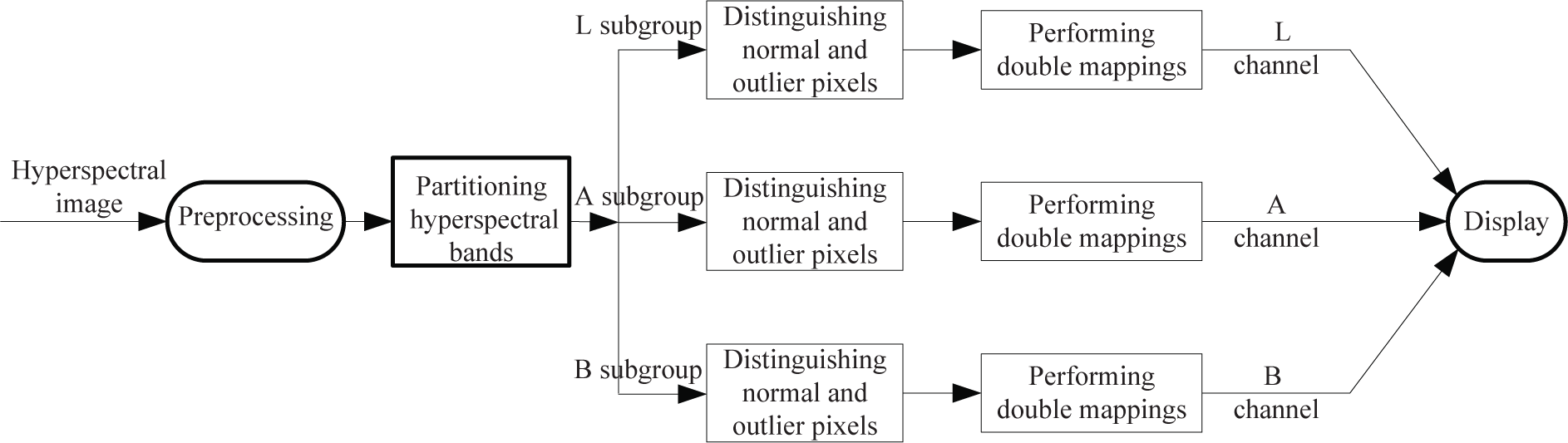
In this section, a new visualization technique for hyperspectral imagery is proposed, i.e., the pairwise-distances-analysis-driven visualization strategy (PDADVS). In this approach, normal pixels and outliers are treated separately using two different mapping methods for enhancing global contrast while avoiding the high risk of sacrificing local details and excessively distorting pairwise distances. For clarity, the flowchart of PDADVS is shown in Figure 5 and detailed descriptions of each step are provided in Sections 3.2 through 3.5.

3.1. Partitioning of Hyperspectral Bands

3.2. Preprocessing

A hyperspectral image generally contains some bad bands (e.g., water absorption and low SNR bands), which impact the following analysis. Therefore, preprocessing is a necessary part of the visualization process. Because of the high-spectral correlation, two adjacent bands in hyperspectral imagery tend to be highly correlated, which conversely provides us a probability to perform the removal of bad bands. Specifically, those bands, whose correlation coefficients to their neighboring bands are less than a given threshold η = 0.8, are removed. Additionally, hyperspectral imagery is affected by additive noise that impairs information extraction and scene interpretation. To reduce this noise, the wavelet hard thresholding approach [28] is applied to each band. Finally, bands with SNR values less than 15dB are excluded.

According to the analysis of pairwise distances in Section 2, we partition all available hyperspectral bands into three subgroups for decreasing the dynamic range of pairwise distances. As such, in terms of the consistency in distance preservation, the relatively smaller dynamic range of pairwise distances in the hyperspectral image space will lead to the smaller gamut of pixels in the color space correspondingly. This is conducive to the feature separability in the sense that the differences between pixels can be better reflected by three color components corresponding to different subgroups respectively rather than these corresponding to the whole band.

To this end, the principle of equal variance is proposed to partition all hyperspectral bands into three subgroups prior to mapping. Different from the equal subgroups technique used in [5,21], equal variance can guarantee that three components of the final color image are correlated (i.e., if the intensity changes, all three components will change accordingly) and the energy is distributed uniformly as in natural color images [29], such that the visualization result is optimal for human visual system. To provide perceptual visualization, three subgroups are then mapped to the device-independent and approximately perceptually uniform CIE (Coherent Infrared Energy) L^∗a^∗b^∗ color space.

To achieve the partitioning, we minimize the following objective function

$${\mathrm{F}}_{s1,s2}={\left(\sigma (U^{I^{1\sim s1}})-\sigma (U^{I^{(s1+1)\sim s2}})\right)}^2+{\left(\sigma (U^{I^{1\sim s1}})-\sigma (U^{I^{(s2+1)\sim r}})\right)}^2+{\left(\sigma (U^{I^{(s1+1)\sim s2}})-\sigma (U^{I^{(s2+1)\sim r}})\right)}^2,s.t0<s1<s2<r$$

(1)

where σ denotes the variance, and $U^{I^{k1~k2}}$ is a $1\times \frac{(w\times h)\times (w\times h-1)}{2}$ row vector for an image of size w × h, corresponding to the Euclidean distances $d_{m,n}^{I^{k1\sim k2}}$ of pairs of spectral vectors in I^k1∼k2. In practice, we consider a subsampling of pairs of pixels in the image (i.e., all pairs with horizontal or vertical displacements of 2^p pixels for p ≥ 3) to compute the vector of pairwise distances for reducing computational complexity. As is well known, there is high relevance between the adjacent-band images in hyperspectral imagery. So each subgroup should consist of contiguous bands in order to keep as much of the common information as possible contained within the subgroup during the mapping. On the other hand, it can be seen from Tables 1 and 2 that both mean and variance of pairwise distances increase with the number of bands in the subgroups. Therefore, a line searching technique is introduced (summarized in Algorithm 1) to solve Equation (1) for the partitioning of hyperspectral bands.

Table 3. Number of the available bands after preprocessing and the partitioning results.

Hyperspectral Images	Number of the Available Bands	Subgroup 1	Subgroup 2	Subgroup 3
Lun.lake01	200	1 ~ 70	71 ~ 127	128 ~ 200
Cuprite02	197	1 ~ 80	81 ~ 123	124 ~ 197
Cuprite03	196	1 ~ 78	79 ~ 130	131 ~ 196
Cuprite04	198	1 ~ 63	64 ~ 116	117 ~ 198
Moffett02_igm	206	1 ~ 33	34 ~ 67	68 ~ 206
Moffett03_igm	216	1 ~ 23	24 ~ 46	47 ~ 216
Lun.lake_igm	207	1 ~ 24	25 ~ 48	49 ~ 207

lists the number of the available bands after preprocessing for all considered experimental hyperspectral images and their partitioning results.

Algorithm 1. Partitioning of hyperspectral bands

Require: I - a hyperspectral image of w × h pixels with r bands;
Ensure: s1, s2 - two splitting points of the whole band
1:	Initialize
2:	k = 0; s1 = ⌊r/3⌋; s2 = 2 × ⌊r/3⌋ + 1;
3:	$U1=\sigma (U^{I^{1\sim s1}});U2=\sigma (U^{I^{(s1+1)\sim s2}});U3=\sigma (U^{I^{(s2+1)\sim r}});$
4:	${\mathcal{F}}_{s1,s2}^{(k)}={(U1-U2)}^2+{(U1-U3)}^2+{(U2-U3)}^2;$
5:	Repeat
6:	σAV = (U1 + U2 + U3)/3;
7:	$step=\lfloor |{\mathcal{F}}_{s1,s2}^{(k)}/10|\rfloor ;$
8:	$if(U1<{\sigma }_{AV})\&(U2<U3),thens1=s1-step;$
9:	$if(U1<{\sigma }_{AV})\&(U2>U3),thens1=s1+step;$
10:	$if(U1>{\sigma }_{AV})\&(U2>U3),thens1=s1-step,s2=s2+2\times step;$
11:	$if(U2<{\sigma }_{AV})\&(U2<U3),thens1=s1+step,s2=s2-2\times step;$
12:	$U1=\sigma (U^{I^{1\sim s1}});U2=\sigma (U^{I^{(s1+1)\sim s2}});U3=\sigma (U^{I^{(s2+1)\sim r}});$
13:	${\mathcal{F}}_{s1,s2}^{(k+1)}={(U1-U2)}^2+{(U1-U3)}^2+{(U2-U3)}^2;$
14:	$△\mathcal{F}=|{\mathcal{F}}_{s1,s2}^{(k+1)}-{\mathcal{F}}_{s1,s2}^{(k)}|$;
15:	k = k + 1;
16:	until △$ℱ$≤10−3

Algorithm 1. Partitioning of hyperspectral bands

Require: I - a hyperspectral image of w × h pixels with r bands;
Ensure: s1, s2 - two splitting points of the whole band
1:	Initialize
2:	k = 0; s1 = ⌊r/3⌋; s2 = 2 × ⌊r/3⌋ + 1;
3:	$U1=\sigma (U^{I^{1\sim s1}});U2=\sigma (U^{I^{(s1+1)\sim s2}});U3=\sigma (U^{I^{(s2+1)\sim r}});$
4:	${\mathcal{F}}_{s1,s2}^{(k)}={(U1-U2)}^2+{(U1-U3)}^2+{(U2-U3)}^2;$
5:	Repeat
6:	σAV = (U1 + U2 + U3)/3;
7:	$step=\lfloor |{\mathcal{F}}_{s1,s2}^{(k)}/10|\rfloor ;$
8:	$if(U1<{\sigma }_{AV})\&(U2<U3),thens1=s1-step;$
9:	$if(U1<{\sigma }_{AV})\&(U2>U3),thens1=s1+step;$
10:	$if(U1>{\sigma }_{AV})\&(U2>U3),thens1=s1-step,s2=s2+2\times step;$
11:	$if(U2<{\sigma }_{AV})\&(U2<U3),thens1=s1+step,s2=s2-2\times step;$
12:	$U1=\sigma (U^{I^{1\sim s1}});U2=\sigma (U^{I^{(s1+1)\sim s2}});U3=\sigma (U^{I^{(s2+1)\sim r}});$
13:	${\mathcal{F}}_{s1,s2}^{(k+1)}={(U1-U2)}^2+{(U1-U3)}^2+{(U2-U3)}^2;$
14:	$△\mathcal{F}=|{\mathcal{F}}_{s1,s2}^{(k+1)}-{\mathcal{F}}_{s1,s2}^{(k)}|$;
15:	k = k + 1;
16:	until △$ℱ$≤10−3

3.3. Outlier Ranking and Detection

As described earlier in Section 2, it is difficult to deal with all pixels of hyperspectral images in the same way for simultaneous discrimination between small and large distances. To address this issue, two different mapping strategies are proposed separately for normal pixels and outlier pixels. This separate approach can achieve the better feature separability with minimum distortion of pairwise distances while avoiding the loss of spatial details.

Prior to performing double mappings, we require to distinguish outliers from normal pixels with the aid of multidimensional scaling (MDS) [30,31]. MDS is a well-known technique for visualizing the high-dimensional data and exploring its underlying structure by analyzing the dissimilarities (or similarities) between pairs of data points, which utilizes an embedding to find coordinates in a low-dimensional space for each high-dimensional data point that preserve the given pairwise dissimilarities as faithfully as possible. Specifically, for each subgroup, the outliers are detected by the following three steps:

Step (1) Given distance matrix $D^{I^{k1\sim k2}}$ with its entry $d_{m,n}^{I^{k1\sim k2}}$ representing the pairwise distance between pixels $I_m^{k1\sim k2}$ and $I_n^{k1\sim k2}$ in a subgroup of hyperspectral imagery, we implement MDS to obtain the coordinates for each pixel of I^k1∼k2 by minimizing the objective function

$${\epsilon }_X={\displaystyle \sum _{m=1}^{w\times h}{\displaystyle \sum _{n=1}^{w\times h}{(d_{m,n}^{I^{k1\sim k2}}-d_{m,n}^{X^{k1\sim k2}})}^2}}$$

(2)

where $d_{m,n}^{I^{k1\sim k2}}=\parallel I_m^{k1\sim k2}-I_n^{k1\sim k2}{\parallel }^2\text{and}{d}_{m,n}^{X^{k1\sim k2}}=\parallel X_m^{k1\sim k2}-X_n^{k1\sim k2}{\parallel }^2$. To calculate the inner product matrix ${(I^{k1\sim k2})}^T{I}^{k1\sim k2}=-\frac{1}{2}J{D}^{I^{k1\sim k2}}J$ with $J=I-\frac{1}{w\times h}e{e}^T$ and e being a column vector of all 1’s [31], now Equation (2) can be reduced to

$${\epsilon }_X^{*}={\displaystyle \sum _{m=1}^{w\times h}{\displaystyle \sum _{n=1}^{w\times h}{\left[{(I_m^{k1\sim k2})}^T{I}_n^{k1\sim k2}-{(X_m^{k1\sim k2})}^T{X}_n^{k1\sim k2}\right]}^2}}$$

(3)

Then the solution for minimizing Equation (3) can be found by solving an eigenvalue problem, given by X^k1∼k2 = Λ^1/2V^T, where Λ is the top q eigenvalues of (I^k1∼k2)^T I^k1∼k2 and V is the eigenvectors of (I^k1∼k2)^T I^k1∼k2 corresponding to the top q eigenvalues.

Step (2) Since the coordinates are computed on the premise of distance preservation, they can be used to measure the degree of deviation of pixels in original high-dimensional space. With the results in Step (1), we define the rank for each pixel of I^k1∼k2, i.e.,

$$rank(I_m^{k1\sim k2})=X_m^{k1\sim k2}-\frac{1}{w\times h}{\displaystyle \sum _{l=1}^{w\times h}{X}_l^{k1\sim k2}}$$

(4)

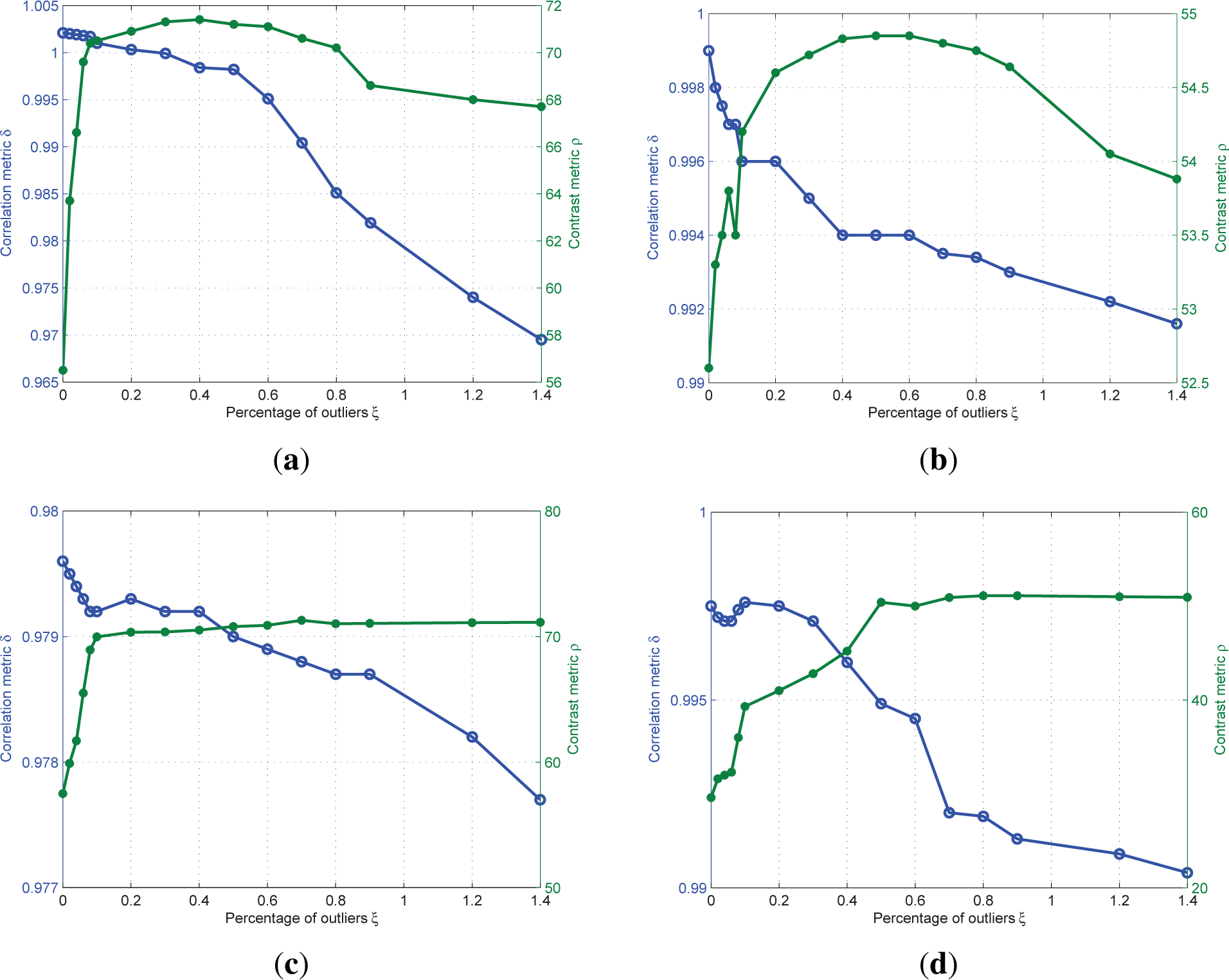
Step (3) Finally, we sort I^k1∼k2 according to their ranks, and then the pixels whose ranks are in the top ξ percent and in the bottom ξ percent should be identified as outliers.

3.4. The Mapping of Normal Pixels

For the hyperspectral image visualization, it is of importance to provide a quick overview for the existing materials and their distribution in the final color image. Moreover, as mentioned in Section 2, the existence of outliers has a negative effect on the feature separability due to their large pairwise distances with normal pixels. As for normal pixels dominating hyperspectral data, it is desirable to keep pairwise distance among them in dimensionality reduction to yield a faithful representation for hyperspectral images.

In terms of the requirements on low computational complexity and the preservation of pairwise distance, we prefer to utilize MDS for the mapping of normal pixels. Here the results is directly extracted from that obtained by MDS in Section 3.3, instead of recalculating the embedded points by defining a new objective function of MDS only involving normal pixels. In such a way, besides simplicity, it is of importance to maintain the consistency of the whole pairwise distances, since normal pixels and outliers will be simultaneously involved in the mapping of outliers in next subsection.

3.5. The Mapping of Outliers

In this subsection, a novel mapping method is proposed for the outliers. This method takes pairwise distance preservation and feature separability into account, and, unlike MDS, adaptively deals with the small and large pairwise distances.

Suppose we have the set ψ of outliers in a subgroup, the objective function for each outlier $I_{m\in \psi }^{k1\sim k2}$ is designed as follows

$${\epsilon }_{P_{m\in \psi }^{k1\sim k2}}=\frac{1}{C}{\displaystyle \sum _{n\in N_s}\frac{{(d_{m,n}^{I^{k1\sim k2}}-d_{m,n}^{P^{k1\sim k2}})}^2}{\sqrt{d_{m,n}^{I^{k1\sim k2}}}}+\mathrm{\lambda }\times \sqrt{d_{m,n}^{I^{k1\sim k2}}}\times d_{m,n}^{P^{k1\sim k2}}}$$

(5)

Where ${\left\{d_{m,n}^{I^{k1\sim k2}}\right\}}_{n\in N_s}$ are the pairwise distances between current outlier $I_m^{k1\sim k2}$ and its neighbors (other outliers or normal pixels), and ${\left\{d_{m,n}^{P^{k1\sim k2}}\right\}}_{n\in N_s}$ are the distances between the embedded point of $I_m^{k1\sim k2}$ in color component P and the neighboring points. $C={\displaystyle {\sum }_{n\in N_s}{d}_{m,n}^{I^{k1\sim k2}}}$, N_s denotes a square fixed-size neighborhood centered around an outlier, and λ is a positive internal parameter balancing the contribution of pairwise distance preservation and feature separability.

The first term ${(d_{m,n}^{I^{k1\sim k2}}-d_{m,n}^{P^{k1\sim k2}})}^2/\sqrt{d_{m,n}^{I^{k1\sim k2}}}$ is used to achieve distance preservation by minimizing the difference of pairwise distances between $d_{m,n}^{I^{k1\sim k2}}$ in hyperspectral image and $d_{m,n}^{P^{k1\sim k2}}$ in the color image. The involving weight $1/\sqrt{d_{m,n}^{I^{k1\sim k2}}}$ is the inverse of the square root of pairwise distance and is designed to enhance the importance of small distances among the neighborhood of outlier $I_{m\in \psi }^{k1\sim k2}$ in the objective function. Correspondingly, small distances are emphasized and local dissimilarity can be preserved in the neighborhood of $P_{m\in \psi }^{k1\sim k2}$ in the color component. Meanwhile, due to large pairwise distances between outliers and normal pixels, a second term is introduced in order to prevent the embeddings of outliers in three color components from departing too far from those that correspond to their respective neighbors. There are two points worth being mentioned about this dimensionality reduction:

• The constraint term in BCOCDM tries to keep the dissimilarity between color pixels. In comparison, the second term of the proposed objective function aims to reduce the deviation between an outlier and its neighbors (especially normal pixels in its neighborhood). This results in a reduction of the color component range. As such, as mentioned in Section 2, more color levels will be used for describing the embedded points associated with normal pixels, which account for the overwhelming majority.
• In order to get good contrast not only in different local regions but also in the full image, the presented method does not simply eliminate or clip the outliers, like the previous algorithms (e.g., PCA2%, and Cui’s [4]). Instead, it adjusts their values in color components based on visualization criteria of pairwise distance preservation and feature separability. As a result, local pairwise distances between outliers and their respective neighbors are preserved, and local information around outliers is also kept.

Algorithm 2. SD algorithm for solving Equation (5)

Require:$P_{m\in \psi /(0)}^{k1\sim k2}$ - initial mapping value of outlier; ϵ - tolerance;
	|Ns| - the size of neighborhood window; Itermax - the maximum number of iterations;
Ensure:$P_{m\in \psi }^{k1\sim k2}$ - the output mapping value of outlier;
1:	Initialize k = 0
2:	repeat
3:	Compute the gradient direction: $$g_m^{(k)}=\nabla {\epsilon }_{P_{m\in \psi /(k)}^{k1\sim k2}}=\frac{-4}{C}{\displaystyle \sum _{n\in N_s}\left[\frac{(d_{m,n}^{I^{k1\sim k2}}-d_{m/(k),n}^{P^{k1\sim k2}})(P_{m/(k)}^{k1\sim k2}-P_n^{k1\sim k2})}{\sqrt{d_{m,n}^{I^{k1\sim k2}}}}-\frac{\mathrm{\lambda }}{2}\times \sqrt{d_{m,n}^{I^{k1\sim k2}}}\times (P_{m/(k)}^{k1\sim k2}-P_n^{k1\sim k2})\right]}$$ (6)
4:	Compute the search direction: ${\beta }_m^{(k)}=-g_m^{(k)}$;
5:	Compute the step length: ${\alpha }_m^{(k)}=\frac{\zeta }{|N_s{|}^2-1}{\Sigma }_{n\in N_s,n\ne m}{d}_{m,n}^{I^{k1\sim k2}}$;
6:	Compute the (k + 1)th iterative value of $P_m^{k1\sim k2}:P_{m/(k+1)}^{k1\sim k2}=P_{m/(k)}^{k1\sim k2}+{\alpha }_m^{(k)}{\beta }_m^{(k)}$;
7:	k = k + 1.
8:	Until$g_m^{(k)}\le \in \text{or}k<Itermax$

Algorithm 2. SD algorithm for solving Equation (5)

Require:$P_{m\in \psi /(0)}^{k1\sim k2}$ - initial mapping value of outlier; ϵ - tolerance;
	|Ns| - the size of neighborhood window; Itermax - the maximum number of iterations;
Ensure:$P_{m\in \psi }^{k1\sim k2}$ - the output mapping value of outlier;
1:	Initialize k = 0
2:	repeat
3:	Compute the gradient direction: $$g_m^{(k)}=\nabla {\epsilon }_{P_{m\in \psi /(k)}^{k1\sim k2}}=\frac{-4}{C}{\displaystyle \sum _{n\in N_s}\left[\frac{(d_{m,n}^{I^{k1\sim k2}}-d_{m/(k),n}^{P^{k1\sim k2}})(P_{m/(k)}^{k1\sim k2}-P_n^{k1\sim k2})}{\sqrt{d_{m,n}^{I^{k1\sim k2}}}}-\frac{\mathrm{\lambda }}{2}\times \sqrt{d_{m,n}^{I^{k1\sim k2}}}\times (P_{m/(k)}^{k1\sim k2}-P_n^{k1\sim k2})\right]}$$ (6)
4:	Compute the search direction: ${\beta }_m^{(k)}=-g_m^{(k)}$;
5:	Compute the step length: ${\alpha }_m^{(k)}=\frac{\zeta }{|N_s{|}^2-1}{\Sigma }_{n\in N_s,n\ne m}{d}_{m,n}^{I^{k1\sim k2}}$;
6:	Compute the (k + 1)th iterative value of $P_m^{k1\sim k2}:P_{m/(k+1)}^{k1\sim k2}=P_{m/(k)}^{k1\sim k2}+{\alpha }_m^{(k)}{\beta }_m^{(k)}$;
7:	k = k + 1.
8:	Until$g_m^{(k)}\le \in \text{or}k<Itermax$

To find the solution of Equation (5), the method of steepest descent (SD) is suggested, for which a quantity, calculated from multiplying the mean of pairwise distances between the outlier and its neighbors by a small scaling factor, is introduced as the step length for improving the convergence speed. This step length will be further adjusted step by step as the solving procedure reaches the best point, so that it fluctuates smoothly and avoids oscillations often arisen in the gradient descent algorithm. The details of SD algorithm for solving Equation (5) are given in Algorithm 2.

4. Experimental Results and Discussion

4.1. Dataset Description and Experimental Setup

To validate the effectiveness of our visualization algorithm, experiments are reported on the hyperspectral image datasets acquired by the National Aeronautics and Space Administration Jet Propulsion Laboratory (AVIRIS) system. These datasets include seven images taken during 1997 from the sites of Lunar Lake (NV), Cuprite (NV), and Moffett Field (CA). They are generated in two different spectral formats: reflectance and radiance. Reflectance images are denoted with a file extension of .rfl while the file extension .igm refers to the radiance images. Two kinds of files both have 224 spectral bands ranging from 400–2500 nm, with nominal bandwidth of 10 nm. For simplification of description, these hyperspectral images will be denoted by Lun.lake₀₁, Cuprite₀₂, Cuprite₀₃, Cuprite₀₄, Moffett₀₂_igm, Moffett₀₃_igm, and Lun.lake_igm, respectively. These image sizes are 512 × 614 pixels.

In this set of experiments, η is set to 0.8 for removing some water absorption bands with the computation of correlation coefficients between adjacent bands, and the strategy described in [21] is used to exclude some low SNR bands in the preprocessing step. Furthermore, the pixels whose ranking values lie within the top and the bottom 0.5 percent (i.e., ξ = 0.5) for the normalized hyperspectral reflectance images and radiance images, are identified as the outliers. These values are found experimentally to have a good compromise for the given data formats are applicable to the multiple test images of each format. In the mapping of outliers, the size of square neighborhood and the internal parameter λ are set to |N_s| = 5 and λ = 1, respectively, as well as ζ = 2 × 10⁻⁴, = 0.001 and Itermax = 40 in the solving procedure. The code for achieving this visualization algorithm runs on MATLAB using an Intel(R) core(XEON) E3 − 1231V3 CPU with 3.40G.

For comparison purpose, visualization performances are evaluated in terms of two metrics: ρ and δ. The correlation-based metric ρ, was proposed in [3,4]. It is the measured correlation between the Euclidean distance of each pairwise spectral vectors in hyperspectral image (denoted as $U_I^{1\sim r}$) and their corresponding pairwise Euclidean distance (color difference) in the perceptual CIE L^∗a^∗b^∗ color space (namely $U_P^{1\sim 3}$). The evaluation of pairwise distance preservation is calculated as follows:

$$\rho =\frac{\frac{{(U_I^{1\sim r})}^T{U}_P^{1\sim 3}}{|U_I^{1\sim r}|}-\overline{U_I^{1\sim r}{U}_P^{1\sim 3}}}{std(U_I^{1\sim r})\cdot std(U_P^{1\sim 3})}$$

(7)

where ${(U_I^{1\sim r})}^T$, $|U_I^{1\sim r}|$, $\overline{U_I^{1\sim r}}$, and $std(U_I^{1\sim r})$ denote the transpose, cardinal, mean, and standard deviation of $U_I^{1\sim d}$, respectively. As suggested in [4], we accelerate this computation by subsampling pixels in practice. In the ideal case, the normalized correlation equals 1. As far as δ is concerned, it is defined as the average pairwise distance between pixels in color space, used to measure the feature separability or contrast:

$$\delta =\frac{|U_P^{1\sim 3}{|}_1}{|U_P^{1\sim 3}|}$$

(8)

in which $|U_P^{1\sim 3}{|}_1$ and $|U_P^{1\sim 3}|$ denote the L₁ norm and the cardinal of vector $U_P^{1\sim 3}$, respectively. In this metric, larger the value of δ represents better feature separability.

4.2. Experimental Results

4.2.1. Parameter Analysis

For the proposed PDADVS algorithm, there are three critical parameters: the percentage of outliers ξ, the size |N_s| of square neighborhood and the internal parameter λ involved in the mapping of outliers. When analyzing one specific parameter, we fix the other parameters as the corresponding values given above. First of all, the effect of different ξ values on the visualization performance is investigated. The score curves of distance preservation and feature separability are shown in Figure 6a,b for Cuprite₀₂ and Cuprite₀₄, in Figure 6c,d for Moffett₀₃_igm and Lun.lake_igm, respectively. From Figure 6, it can be seen that the score of pairwise distance preservation (indicating by the blue curve) slowly decreases with the increase of ξ on the whole for four hyperspectral images. Concerning the score of feature separability, one can observe from Figure 6a–d that the contrasts are monotonically increasing at the beginning (i.e., ξ is less than about 0.5), but the results progressively worsen with the further increase of ξ, possibly caused by the overadjustment over normal pixels. By considering the tradeoff between distance preservation and feature separability, ξ is suggested to be set as 0.5 for the reflectance and radiance hyperspectral images in all the following experiments.

In addition to the quantitative comparison, we also take the Lun.lake_igm as an example for visual interpretation. Figure 7 illustrates three color visualization results of Lun.lake_igm obtained by the proposed PDADVS model with ξ = 0, 0.5, 5, respectively. In Figure 7a, the image is relatively dark in that some pairwise distances between the outliers and their respective neighbors may not be sufficiently adjusted while there appears to have colors pop-outed (indicated by red ellipse areas) by the overadjustment over normal pixels and some textures become indistinct in Figure 7c. Only in Figure 7b, features can be easily identified and more fine details are visible due to the appropriate choice of ξ.

Furthermore, the neighboring window size |N_s| is also tested on the hyperspectral image of Lun.lake_igm.

Table 4. Scores of both metrics and running time obtained by the PDADVS model involving different values of |N_s| with keeping ξ = 0.5 and λ = 1 for Lun.lake_igm.

|Ns|	ρ	δ	Running Time in Seconds
3	0.9972	59.1	6.8
5	0.9950	64.1	11.5
7	0.9888	71.0	15.1
9	0.9771	72.4	26.2
11	0.9525	73.1	38.6

lists the scores of both metrics and the running time. According to Table 4, the comparisons indicate that |N_s| has a positive impact on the running time, but the pairwise distance preservation slightly decreases as |N_s| increases while the contrast cannot be further improved when the value of |N_s| is larger than 7. By making comprehensive consideration for performance and complexity, we suggest that |N_s| = 5 is chosen in practice.

Finally, another parameter λ related to the mapping of outliers is also studied, which controls the contribution of pairwise distance preservation and feature separability. To this end, we roughly choose λ in the range [0, 1, 2, 3, 4, 5]. The ρ and δ scores evaluated on all experimental hyperspectral images are given in

Table 5. ρ and δ scores obtained by the PDADVS model for increasing values of λ.

Hyperspectral images	λ = 0	λ = 1	λ = 2	λ = 3	λ = 4	λ = 5
Lun.lake01	0.991 [50.1]	0.986 [60.8]	0.982 [67.4]	0.974 [69.5]	0.956 [70.1]	0.942 [71.3]
Cuprite02	0.997 [55.0]	0.996 [69.2]	0.990 [75.1]	0.982 [77.2]	0.973 [78.1]	0.963 [78.8]
Cuprite03	0.997 [38.2]	0.992 [44.2]	0.985 [54.9]	0.980 [56.2]	0.978 [57.8]	0.970 [58.1]
Cuprite04	0.998 [46.1]	0.996 [54.8]	0.994 [58.1]	0.986 [62.9]	0.980 [64.9]	0.976 [66.3]
Moffett02_igm	0.990 [62.1]	0.985 [68.3]	0.980 [71.3]	0.975 [72.0]	0.961 [73.5]	0.952 [74.3]
Moffett03_igm	0.985 [67.5]	0.981 [70.8]	0.971 [72.5]	0.963 [73.1]	0.951 [73.8]	0.942 [74.5]
Lun.lake_igm	0.997 [58.2]	0.995 [64.1]	0.988 [67.3]	0.982 [70.1]	0.979 [71.4]	0.961 [72.4]

. As expected, the results show that, as λ increases from 0 to 5, there is an obvious improvement on contrast but being subjected to the detriment of the preservation of pairwise distance. This indicates that the introduction of the constraint term in Equation (5) is helpful to the contrast enhancement. By a comprehensive analysis, λ = 1 is an acceptable choice which can provide the satisfactory contrast on the premise of guaranteeing ρ > 0.980 for all these hyperspectral images.

4.2.2. Quantitative Comparison

To validate our proposed PDADVS, we compare it with several existing visualization algorithms: CMF [3], PCA [4], PCA2% [4], and BCOCDM [5].

Table 6. Comparison of correlation ρ and contrast δ obtained by all considered visualization algorithms.

Hyperspectral Images	CMF	PCA	PCA2%	BCOCDM	PDADVS
Lun.lake01	0.823 [5.6]	0.920 [10.9]	0.532 [52.5]	0.984 [17.6]	0.986 [60.8]
Cuprite02	0.881 [7.7]	0.953 [13.9]	0.432 [53.3]	0.971 [17.5]	0.996 [69.2]
Cuprite03	0.802 [13.9]	0.910 [10.2]	0.585 [45.1]	0.966 [20.8]	0.992 [44.2]
Cuprite04	0.813 [8.4]	0.903 [10.5]	0.413 [47.3]	0.951 [13.0]	0.996 [54.3]
Moffett02_igm	0.871 [12.8]	0.961 [11.2]	0.551 [78.5]	0.948 [26.5]	0.985 [68.3]
Moffett03_igm	0.864 [10.1]	0.966 [13.2]	0.602 [47.8]	0.959 [18.8]	0.981 [70.8]
Lun.lake_igm	0.896 [16.4]	0.945 [12.3]	0.554 [41.4]	0.984 [17.6]	0.995 [64.1]

reports the quantitative results measured on the test hyperspectral images for all considered algorithms.

From Table 6, the comparison of ρ and δ values shows that CMF is less competitive than other methods. As expected, BCOCDM outperforms PCA for most cases in pairwise distance preservation and separability of features, both of which have the higher ρ values and the relatively lower δ ones. This phenomenon manifests that feature details in the color image may not be discriminated when the preservation of distance metric is the main focus of BCOCDM or is the only purpose as done in PCA. Conversely, PCA2% with the highest δ values yields the best contrast but gives a lower score for ρ, which indicates that pairwise distances are distorted seriously in the final color image. This probably results in an unreliable interpretation for hyperspectral images. Meanwhile still from this Table, we can clearly observe that our proposed PDADVS provides the best performance in pairwise distance preservation, as it is comparable to PCA2% in terms of contrast with the δ values being about four times larger than that of PCA. From an overall perspective, PDADVS performs best and can obtain the better contrast at the smallest cost of sacrificing distance preservation.

Furthermore, visualization results of Moffett₀₃_igm and Moffett₀₂_igm (both with a size of 512× 614) obtained by PCA, BCOCDM, PDAVDS, and PCA%2 are shown in Figures 8 and 9 for a visual comparison. It can be observed from Figures 8 and 9 that different regions can be easily identified, and very fine details (e.g., that pointed by red arrows in Figure 8, and buildings in the Moffett₀₂_igm scene) are clearly visible even if in relatively dark or bright local areas, which is consistent with the quantitative results. For other methods, there always exist areas in which some colors “pop out” to different extent or the color is so dark that details in these local areas may not be distinguished. Moreover, Figure 10 gives the color displays of four reflectance scenes, obtained by our proposed PDADVS. In this figure, all images exhibit a natural color looking.

5. Discussion

In terms of visualization effectiveness, our proposed PDADVS is superior to other state-of-the-art algorithms for all the hyperspectral images, whose good performance mainly comes from the separate treatment of outliers. By doing so, the gap between color pixels in the mapped color space corresponding to outliers and normal pixels can be decreased such that the pixel diversity is achieved, on the premise of preserving pairwise distances. As such, it is very suitable for handling the hyperspectral images with more complicated geographical features. On the contrary, a possible limitation of the proposed method is that it is not too effective in the hyperspectral images whose scenes are relative simple. For example, from Table 6 we can see that the proposed PDADVS with the same parameter settings yields the higher δ values for Moffett₀₂_igm, Moffett₀₃_igm and Cuprite₀₂ than Lun.lake₀₁, Cuprite₀₃, Cuprite₀₄, and Lun.lake_igm.

As further remarks, it is worth noting that, although the above experimental analysis is performed on the portions of the original hyperspectral images, this technique can be used to the large images. To illustrate the applicability, we test the performance of PDADVS on the original images of Moffett₀₂_igm and Moffett₀₃_igm, respectively, having 2032×614 and 1924×753 pixels. It allows achieving ρ = 0.981, δ = 61.3 for Moffett₀₂_igm and ρ = 0.980, δ = 50.3 for Moffett₀₃_igm. The running times are 56.4 and 56.2 seconds for Moffett₀₂_igm and Moffett₀₃_igm, respectively. Figure 11 shows their corresponding visualization results, which provide evidence for good performance of PDADVS. From Figure 11, it is interesting to observe that the different regions as well as man-made structures and objects are still clearly identifiable in these two images.

In addition, we discuss the computational complexity of the PDADVS algorithm. Specifically, the embedded points corresponding to normal pixels are obtained through calculating eigenvalues and eigenvectors, whose computational time is less than a millisecond. So we don’t care about the running time of the mapping of normal pixels. On the other hand, the mapping of outliers is a spring system [24]. Each outlier is linked to its neighborhood through springs whose lengths correspond to the pairwise distances between the outlier and its neighbors in the original space. In this way, we place the outliers in the output space and keep the pairwise distances between the embedded points of outliers and their respective neighbors as similar as possible to those in the original space. The implementation of the mapping for the outliers would require the computational complexity O(|N_S| × Itermax × O_N) (O_N is the number of outliers). As mentioned above, the number of outliers takes a very small proportion of pixels in hyperspectral image (e.g., 0.5 even less). Compared with other algorithms using nonlinear mapping for all pixels such as BCOCDM, the computational complexity of the mapping in our algorithm is greatly reduced. For example, if the outliers are about 0.5% of all pixels, the running time of our method should reduce to about 0.5% of the BCOCDM’s.

6. Conclusion

In this paper, a novel pairwise-distances-analysis-driven visualization strategy (PDADVS) is proposed for the visualization of hyperspectral imagery. The analysis of pairwise distances reveals that the dimensionality of the original data space influences both the dynamic range and variance or the larger pairwise distances and outliers negatively affect the visualization of pixel diversity (i.e., contrast). From this perspective, the proposed selection of band subgroups, using the principle of equal variance, improves the ability to map hyperspectral imagery such that the visualization is close to a natural image and makes the resulting color image more suitable for the perception by the human visual system. Additionally, the proposed dual mapping technique, used to separately map normal and outlier pixels to the CIE L^∗a^∗b^∗ color space, preserves pairwise distances as much as possible while maintaining good contrast both regionally and across the full image. In particular, the objective function involves the weighting of pairwise distances in the mapping of outliers and adaptively retains local information in the neighborhood of each outlier.

Experimental results reported on several AVIRIS hyperspectral images show that the proposed PDADVS yields the better overall performance, and is a fast and efficient technique for the visualization of hyperspectral image.