
Hyperspectral REE (Rare Earth Element) Mapping of Outcrops—Applications for Neodymium Detection

Abstract
:
1. Introduction
1.1. Introduction to Hyperspectral Data Acquisition
1.2. Introduction to Imaging Spectroscopy Principles for the Classification of Rare Earth Element Bearing Minerals and Rocks
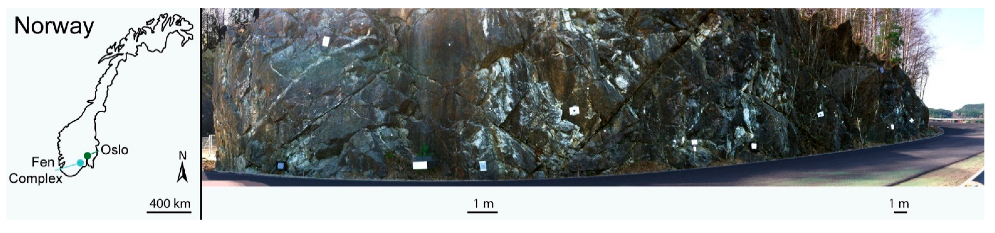
2. Geological Setting

3. Methods
3.1. Remote Sensing Analyses
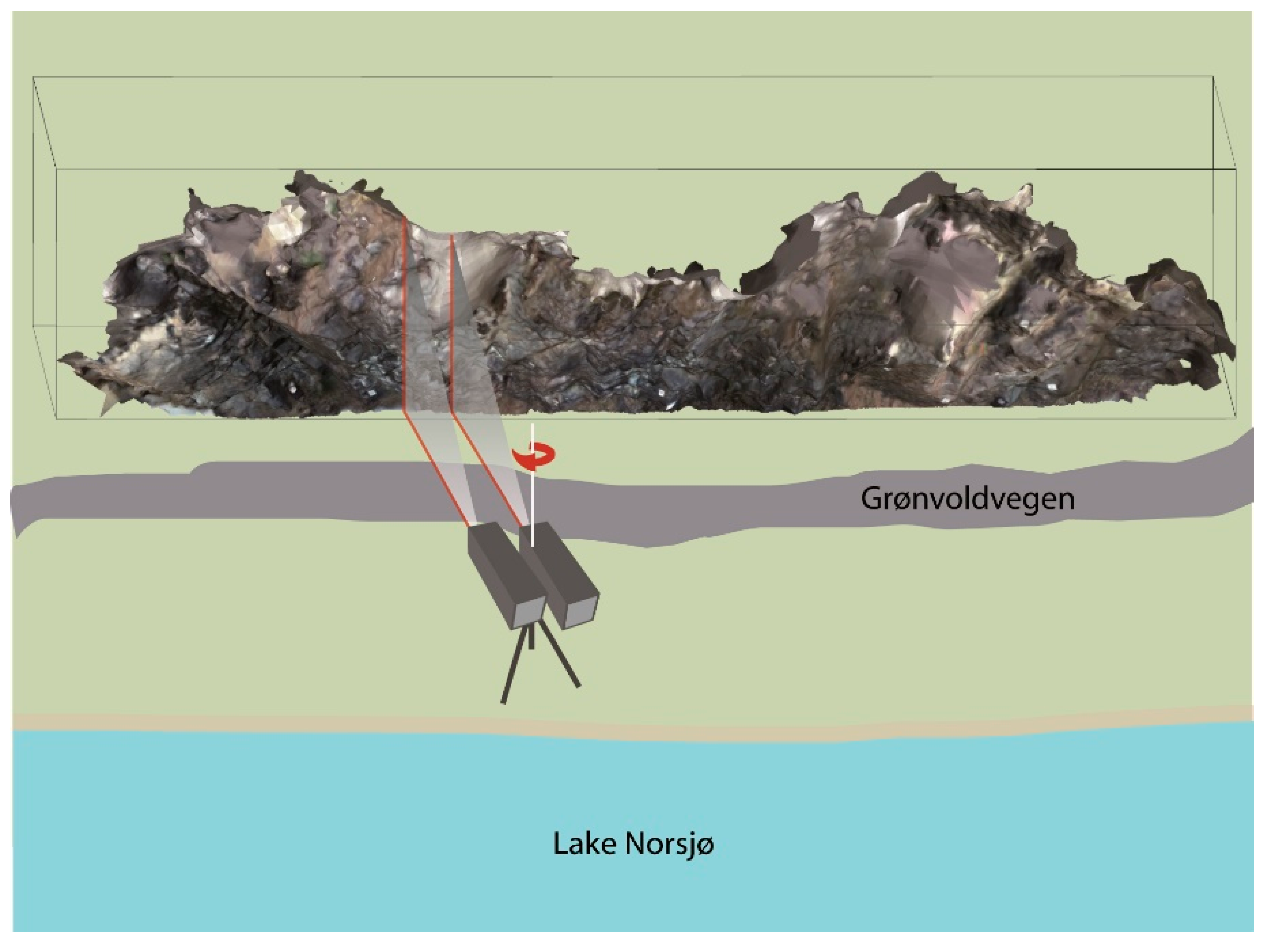
3.1.1. Instruments and Fieldwork Procedure

| Camera | VNIR | SWIR |
|---|---|---|
| Integration time (ms) | 30 | 30 |
| Frame period (ms) | 31 | 61.753 |
| Frames (#) | 4000 | 1110 |
| Field of view (°) | 34 1 | 27 1 |
| Spectral sampling interval (nm) | 3.7 | 6 |
| Radiometric resolution (bit) | 12 | 14 |
| Bands (#) | 160 | 256 |
| Detectors (pixel) | 1600 | 320 |
3.1.2. Brief Description of the Proposed Approach
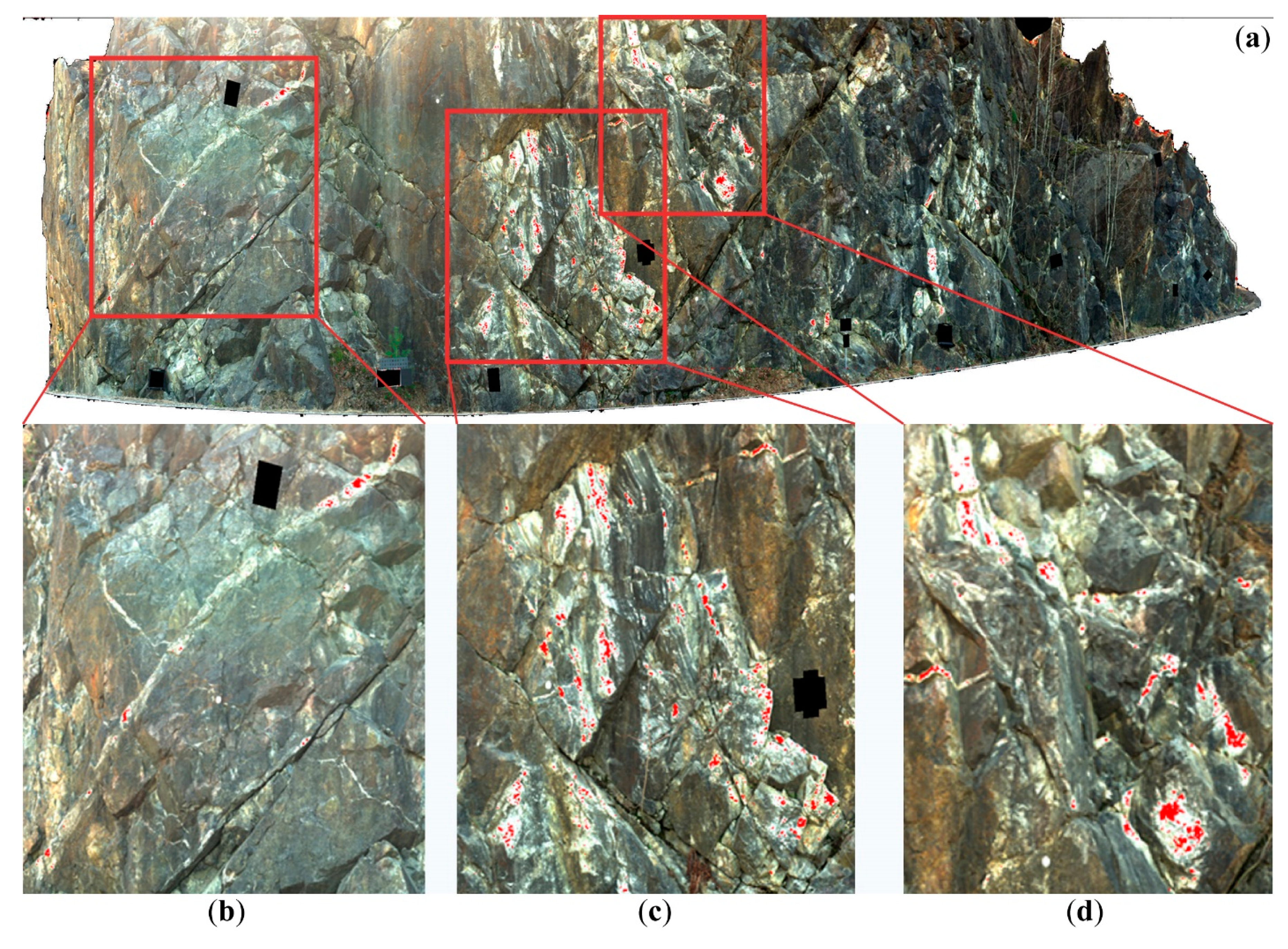
3.1.3. Proposed Approach
3.2. Geochemical Analysis Tools for Retrieving Complimentary Information
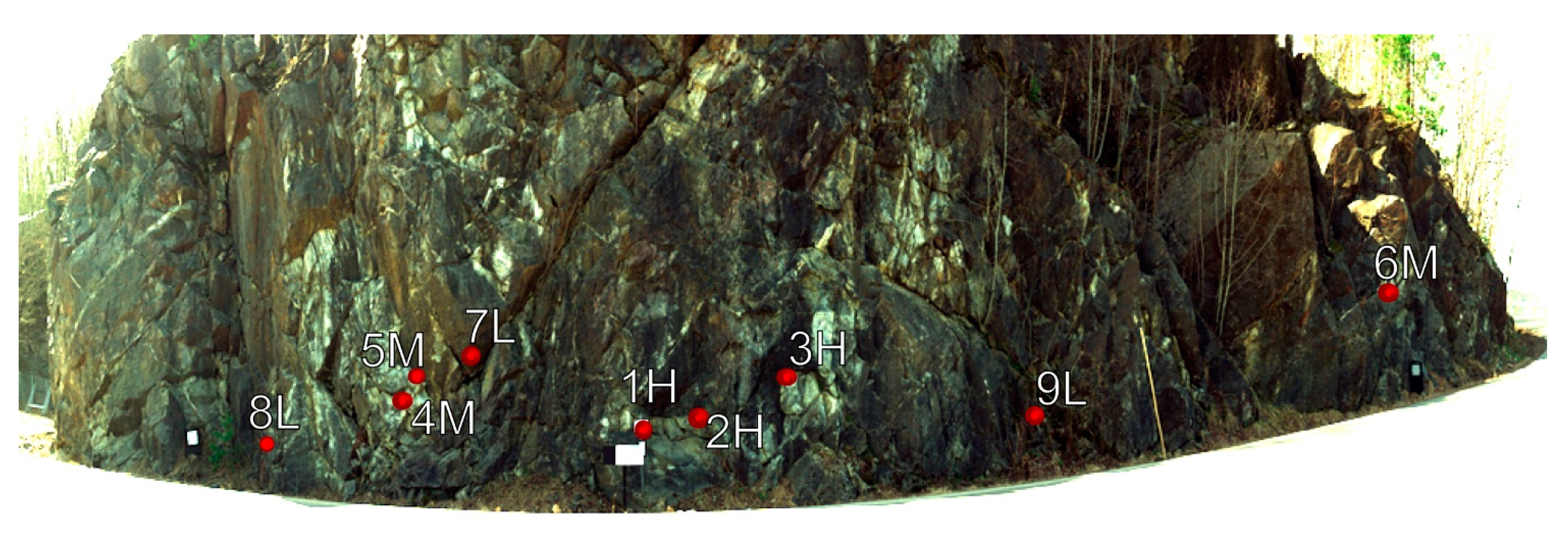
3.2.1. Brief Theoretical Background of the Geochemical Methods and Sampling Design

3.2.2. Realization and Instrumentation for Chemical Analysis

4. Results
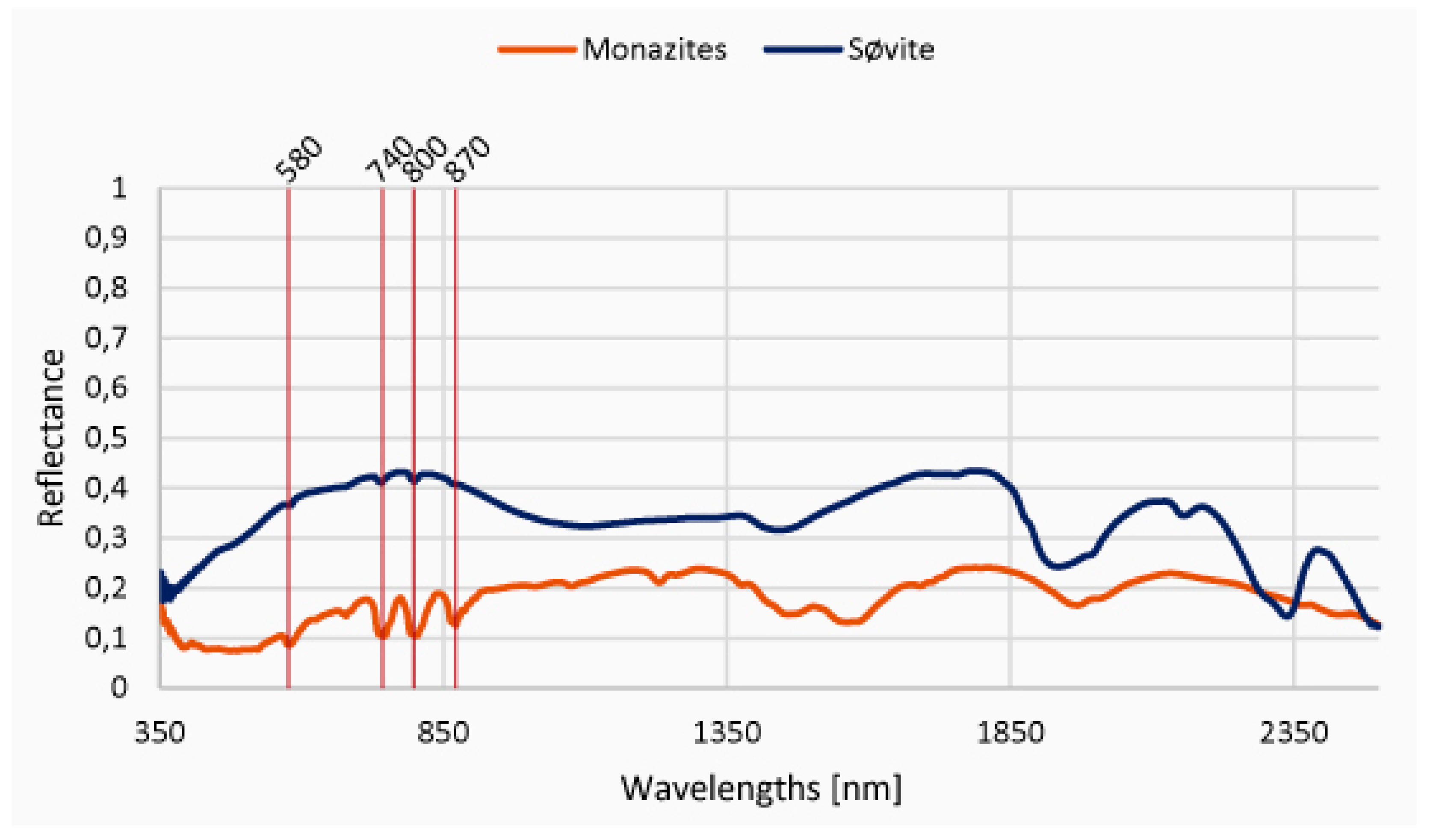
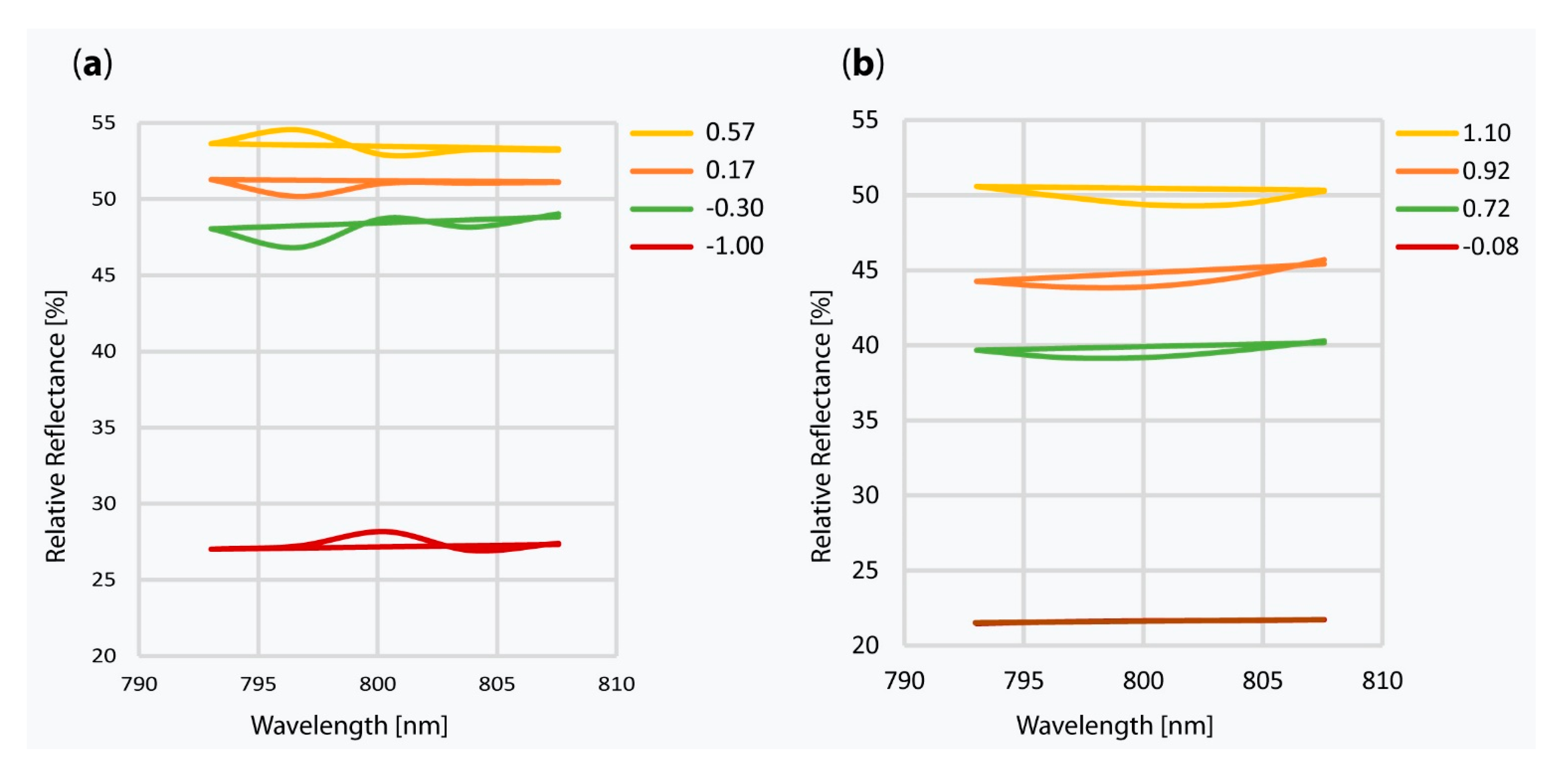
4.1. Spectroscopy
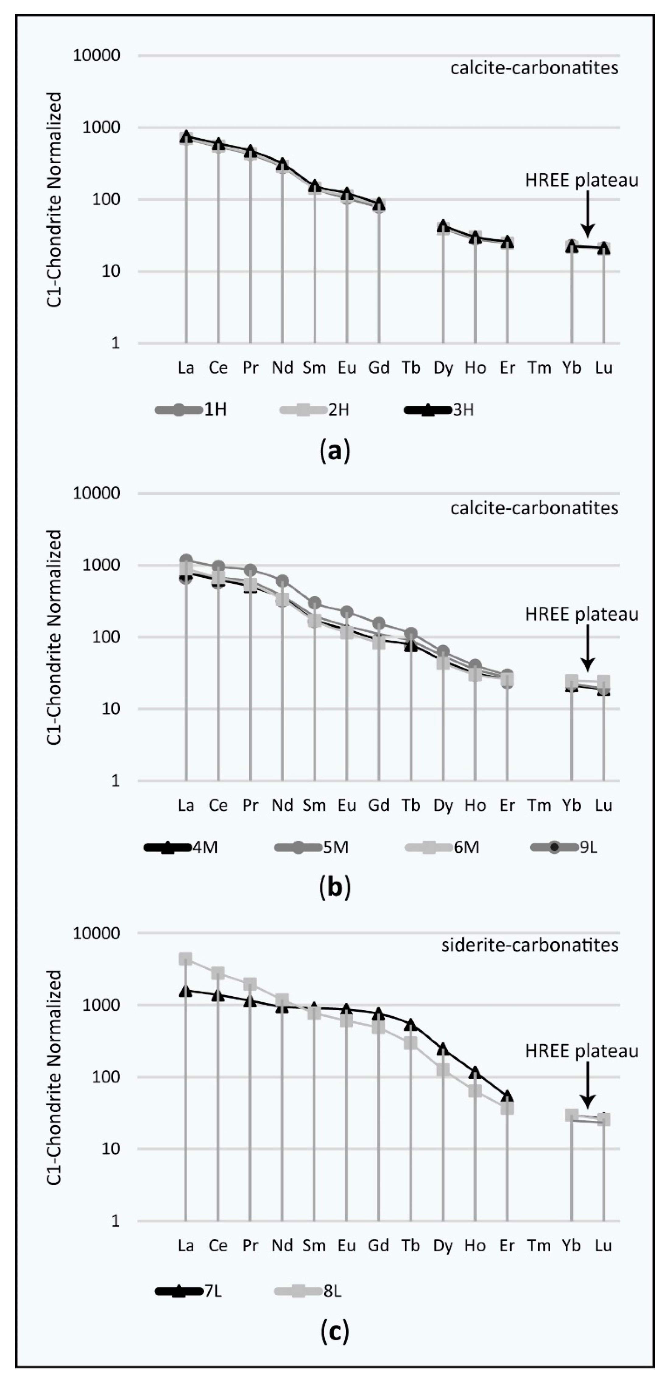
4.2. Chemistry and Mineralogy

| C1-Chondrite | 1H | 2H | 3H | 4M | 5M | 6M | 7L | 8L | 9L | |
|---|---|---|---|---|---|---|---|---|---|---|
| Y | N/A | 48 | 49 | 51 | 53 | 61 | 50 | 168 | 89 | 58 |
| La | 0.237 | 164 | 167 | 179 | 186 | 278 | 212 | 377 | 1032 | 186 |
| Ce | 0.612 | 330 | 338 | 367 | 383 | 587 | 413 | 845 | 1699 | 413 |
| Pr | 0.095 | 40 | 41 | 45 | 48 | 81 | 51 | 109 | 185 | 58 |
| Nd | 0.467 | 130 | 135 | 146 | 161 | 282 | 157 | 442 | 550 | 178 |
| Sm | 0.153 | 22 | 22 | 24 | 27 | 46 | 26 | 138 | 118 | 30 |
| Eu | 0.058 | 6 | 6.5 | 7.1 | 7.4 | 13 | 6.7 | 50 | 35 | 8.3 |
| Gd | 0.2055 | 16 | 17 | 18 | 19 | 32 | 17 | 155 | 100 | 23 |
| Tb | 0.0374 | N/A | N/A | N/A | 2.9 | 4.2 | N/A | 20 | 11 | 3.4 |
| Dy | 0.254 | 10 | 10 | 11 | 12 | 16 | 11 | 62 | 32 | 14 |
| Ho | 0.0566 | 1.6 | 1.7 | 1.7 | 1.8 | 2.3 | 1.7 | 6.6 | 3.6 | 2.0 |
| Er | 0.1655 | 4.1 | 4.1 | 4.3 | 4.3 | 4.9 | 4.3 | 8.9 | 6.1 | 4.6 |
| Tm | 0.0255 | N/A | N/A | N/A | N/A | N/A | N/A | N/A | N/A | N/A |
| Yb | 0.17 | 3.9 | 3.7 | 3.8 | 3.6 | 3.8 | 4.2 | 5.0 | 5.0 | 4.2 |
| Lu | 0.0254 | 0.54 | 0.52 | 0.54 | 0.48 | 0.49 | 0.61 | 0.67 | 0.65 | 0.59 |
| Sc | N/A | 2.2 | 2 | 3.6 | 2.1 | 2.9 | 3.7 | 74 | 33 | 5.3 |
| Reading No. | 1H | 2H | 3H | 4M | 5M | 6M | 7L | 8L | 9L |
|---|---|---|---|---|---|---|---|---|---|
| Duration of measurement (s) | 122.79 | 124.86 | 132.57 | 123.58 | 121.99 | 120.58 | 124.35 | 123.32 | 123.38 |
| Units | ppm | ppm | ppm | ppm | ppm | ppm | ppm | ppm | ppm |
| Nb | 2493.48 | 1155.47 | 1694.60 | 2094.15 | 2963.61 | 521.13 | 4748.08 | 1578.00 | 1447.73 |
| Y | 62.31 | 59.15 | 58.60 | 63.69 | 71.98 | 58.74 | 176.11 | 111.74 | 64.98 |
| Th | <LOD | <LOD | <LOD | <LOD | <LOD | <LOD | <LOD | 480.00 | <LOD |
| U | <LOD | <LOD | <LOD | <LOD | <LOD | <LOD | 121.81 | <LOD | <LOD |
| Units | percent | percent | percent | percent | percent | percent | percent | percent | percent |
| Fe | 0.64 | 0.26 | 0.38 | 0.29 | 0.67 | 0.38 | 3.87 | 4.50 | 0.84 |
| Ca | 43.35 | 43.24 | 43.33 | 43.69 | 41.39 | 43.29 | 32.32 | 36.23 | 42.56 |
| K | 0.16 | 0.06 | 0.12 | <LOD | 0.09 | <LOD | 0.13 | 0.09 | 0.06 |
| S | 0.13 | <LOD | <LOD | <LOD | 0.08 | <LOD | 0.44 | 1.05 | 0.23 |
| P | 0.24 | 0.34 | 0.55 | 0.70 | 2.46 | 0.20 | 1.03 | 0.41 | 0.44 |
| Si | 1.03 | 0.66 | 1.25 | 0.44 | 1.03 | 0.43 | 1.17 | 0.81 | 0.77 |
| Cl | 0.01 | 0.01 | 0.01 | <LOD | 0.01 | 0.01 | 0.01 | 0.01 | 0.02 |
| Mn | 0.31 | 0.24 | 0.35 | 0.26 | 0.43 | 0.47 | 0.54 | 0.42 | 0.36 |
| Al | <LOD | <LOD | <LOD | <LOD | <LOD | <LOD | <LOD | <LOD | <LOD |
| Mg | <LOD | <LOD | <LOD | <LOD | <LOD | <LOD | <LOD | <LOD | <LOD |
| Not detectable | 52.91 | 53.99 | 52.72 | 53.53 | 52.67 | 54.28 | 57.42 | 54.99 | 53.98 |
| Total | 99.21 | 99.10 | 99.04 | 99.33 | 99.40 | 99.29 | 97.75 | 99.12 | 99.52 |
| Element Oxide | Average Weight Percent of 19 Monazite Measurements |
|---|---|
| P2O5 | 30.05 |
| CaO | 0.79 |
| SiO2 | 0.35 |
| Al2O3 | 0.04 |
| FeO | 0.36 |
| Y2O3 | 0.12 |
| La2O3 | 12.98 |
| Ce2O3 | 31.83 |
| Nd2O3 | 15.61 |
| Pr2O3 | 4.00 |
| Sm2O3 | 1.81 |
| Gd2O3 | 0.60 |
| Tb2O3 | 0.03 |
| Dy2O3 | 0.08 |
| Ho2O3 | 0.01 |
| Er2O3 | 0.03 |
| Yb2O3 | 0.01 |
| Lu2O3 | <LOD |
| ThO2 | 0.22 |
| UO2 | <LOD |
| PbO | 0.02 |
| Total | 98.94 |
5. Discussion
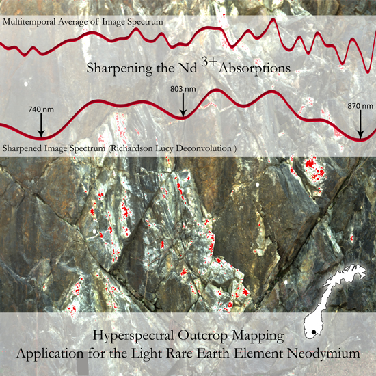
5.1. Validation of the Proposed Method, the Richardson Lucy Deconvolution and the Multitemporal Approach


5.2. Discussion of the Results from the Introduced New Method and their Chemical Evaluation


6. Conclusions
Acknowledgments
Author Contributions
Conflicts of Interest
References
- Laznicka, P. Giant Metallic Deposits; Springer Berlin Heidelberg: Berlin/Heidelberg, Germany, 2010. [Google Scholar]
- Xu, C.; Wang, L.; Song, W.; Wu, M. Carbonatites in China: A review for genesis and mineralization. Geosci. Front. 2010, 1, 105–114. [Google Scholar] [CrossRef]
- Rogass, C.; Spengler, D.; Bochow, M.; Segl, K.; Lausch, A.; Doktor, D.; Roessner, S.; Behling, R.; Wetzel, H.U.; Kaufmann, H. Reduction of radiometric miscalibration—Applications to pushbroom sensors. Sensors 2011, 11, 6370–6395. [Google Scholar] [CrossRef] [PubMed]
- Clark, R.N.; Swayze, G.A.; Livo, K.E.; Kokaly, R.F.; Sutley, S.J.; Dalton, J.B.; McDougal, R.R.; Gent, C.A. Imaging spectroscopy: Earth and planetary remote sensing with the USGS Tetracorder and expert systems. J. Geophys. Res. 2003. [Google Scholar] [CrossRef]
- Rowan, L.C.; Kingston, M.J.; Crowley, J.K. Spectral reflectance of carbonatites and related alkalic igneous rocks; selected samples from four North American localities. Econ. Geol. 1986, 81, 857–871. [Google Scholar] [CrossRef]
- Rowan, L.C.; Mars, J.C. Lithologic mapping in the Mountain Pass, California area using advanced spaceborne thermal emission and reflection radiometer (ASTER) data. Remote Sens. Environ. 2003, 84, 350–366. [Google Scholar] [CrossRef]
- Momose, A.; Miyatake, S.; Arvelyna, Y.; Nguno, A.; Mhopjeni, K.; Sibeso, M.; Muyongo, A.; Muvangua, E. Mapping pegmatite using HyMap data in southern Namibia. In Proceedings of the 2011 IEEE International Geoscience and Remote Sensing Symposium (IGARSS), Vancouver, BC, Canada, 2011; pp. 2216–2217.
- Hernandez, E.A.; Filho, C.R. Spectral reflectance and eissivity features of PO4-bearing carbonatitic rocks from the Catalão I and Tapira complexes: New constraints for detection of igneous phosphates with remote sensing data. In Proceedings of the Anais XVI Simpósio Brasileiro de Sensoriamento Remoto-SBSR, Foz do Iguaçu, Brasil, 13–18 April 2013.
- Bedini, E. Mapping lithology of the Sarfartoq carbonatite complex, southern West Greenland, using HyMap imaging spectrometer data. Remote Sens. Environ. 2009, 113, 1208–1219. [Google Scholar] [CrossRef]
- Dai, J.; Wang, D.; Wang, R.; Chen, Z. Quantitative estimation of concentrations of dissolved rare earth elements using reflectance spectroscopy. J. Appl. Remote Sens. 2013, 7. [Google Scholar] [CrossRef]
- Bedini, E.; Tukiainen, T. Using spectral mixture analysis of hyperspectral remote sensing data to map lithology of the Sarfartoq carbonatite complex, southern West Greenland. Geol. Surv. Den. Greenl. Bull. 2009, 17, 69–72. [Google Scholar]
- Van der Meer, F.D.; van der Werff, H.M.A.; van Ruitenbeek, F.J.A.; Hecker, C.A.; Bakker, W.H.; Noomen, M.F.; van der Meijde, M.; Carranza, E.J.M.; de Smeth, J.B.; Woldai, T. Multi- and hyperspectral geologic remote sensing: A review. Int. J. Appl. Earth Obs. Geoinf. 2012, 14, 112–128. [Google Scholar] [CrossRef]
- Cloutis, E.A. Hyperspectral geological remote sensing: Evaluation of analytical techniques. Int. J. Remote Sens. 1996, 17, 2215–2242. [Google Scholar] [CrossRef]
- Mielke, C.; Boesche, N.K.; Rogass, C.; Kaufmann, H.; Gauert, C.; de Wit, M. Spaceborne mine waste mineralogy monitoring in South Africa, applications for modern push-broom missions: Hyperion/OLI and EnMAP/Sentinel-2. Remote Sens. 2014, 6, 6790–6816. [Google Scholar] [CrossRef]
- Townsend, T.E. Discrimination of iron alteration minerals in visible and near-infrared reflectance data. J. Geophys. Res. 1987, 92, 1441–1454. [Google Scholar] [CrossRef]
- White, W.B. Diffuse-reflectance spectra of rare-earth oxides. Appl. Spectrosc. 1967, 21, 167–171. [Google Scholar] [CrossRef]
- Dieke, G.H.; Crosswhite, H.M. The spectra of the doubly and triply ionized rare earths. Appl. Opt. 1963, 2, 675–686. [Google Scholar] [CrossRef]
- Williams, M.L.; Jercinovic, M.J.; Harlov, D.E.; Budzyń, B.; Hetherington, C.J. Resetting monazite ages during fluid-related alteration. Chem. Geol. 2011, 283, 218–225. [Google Scholar] [CrossRef]
- ASD Inc Field Spec 3 HR (Build in 2010). Available online: http://www.sphereoptics.de/en/spectrometers/docs/Field%20Spec%203%20HR%202010.pdf (accessed on 1 April 2015).
- Leonard, J.P.; Nolan, C.B.; Stomeo, F.; Gunnlaugsson, T. Photochemistry and photophysics of coordination compounds: Lanthanides. Top. Curr. Chem. 2007, 281, 1–43. [Google Scholar]
- Kumar, G.A.; Riman, R.E.; Diaz Torres, L.A.; Banerjee, S.; Romanelli, M.D.; Emge, T.J.; Brennan, J.G. Near-infrared optical characteristics of chalcogenide-bound Nd3+ molecules and clusters. Chem. Mater. 2007, 19, 1610–1620. [Google Scholar]
- Turner, D.J.; Rivard, B.; Groat, L.A. Visible and short-wave infrared reflectance spectroscopy of REE fluorocarbonates. Am. Mineral. 2014, 99, 1335–1346. [Google Scholar] [CrossRef]
- Boesche, N.K.; Rogaß, C.; Mielke, C.; Kaufmann, H. Hyperspectral digital image analysis and geochemical analysis of a rare earth elements mineralized intrusive complex (fen carbonatite complex in Telemark region, Norway). In Proceedings of 34th EARSeL Symposium, Warsaw, Poland, 16–20 June 2014.
- Ramberg, D.I.B. Gravity studies of the Fen complex, Norway, and their petrological significance. Contrib. Mineral. Petrol. 1973, 38, 115–134. [Google Scholar] [CrossRef]
- Mitchell, R.H.; Brunfelt, A.O. Rare earth element geochemistry of the Fen alkaline complex, Norway. Contrib. Mineral. Petrol. 1975, 52, 247–259. [Google Scholar] [CrossRef]
- Andersen, T. Evolution of peralkaline calcite carbonatite magma in the Fen complex, southeast Norway. Lithos 1988, 22, 99–112. [Google Scholar] [CrossRef]
- Andersen, T. Magmatic fluids in the Fen carbonatite complex, S.E. Norway. Contrib. Mineral. Petrol. 1986, 93, 491–503. [Google Scholar] [CrossRef]
- Lie, A.; Ostergaard, C. The Fen carbonatite complex, Ulefoss, Norway; 21st NORTH: Svendborg, Denmark, 2011. [Google Scholar]
- Norsk Elektro Optikk. HySpex VNIR 1600/SWIR320 m-e. Available online: http://www.sphereoptics.de/de/spektrometer/docs/HySpex-GenerellMail.pdf (accessed on 1 April 2015).
- Sunshine, J.M.; Pieters, C.M.; Pratt, S.F. Deconvolution of mineral absorption bands: An improved approach. J. Geophys. Res.: Solid Earth 1990, 95, 6955–6966. [Google Scholar] [CrossRef]
- Ben-Dor, E.; Chabrillat, S.; Demattê, J.A.M.; Taylor, G.R.; Hill, J.; Whiting, M.L.; Sommer, S. Using imaging spectroscopy to study soil properties. Remote Sens. Environ. 2009, 113, S38–S55. [Google Scholar] [CrossRef]
- Guanter, L.; Richter, R.; Moreno, J. Spectral calibration of hyperspectral imagery using atmospheric absorption features. Appl. Opt. 2006, 45, 2360–2370. [Google Scholar] [CrossRef] [PubMed]
- Harsdorf, S.; Reuter, R. Stable deconvolution of noisy lidar signals. In Proceedings of 2000 EARSeL-SIG-Workshop, Dresden, Germany, 16–17 June 2000.
- Sunshine, J.M.; Pieters, C.M. Estimating modal abundances from the spectra of natural and laboratory pyroxene mixtures using the modified Gaussian model. J. Geophys. Res.: Planets 1993, 98, 9075–9087. [Google Scholar] [CrossRef]
- Zuleger, E.; Erzinger, J. Determination of the REE and Y in silicate materials with ICP-AES. Fresenius’ Z. Anal. Chem. 1988, 332, 140–143. [Google Scholar] [CrossRef]
- Sun, S.-S.; McDonough, W.F. Chemical and isotopic systematics of oceanic basalts: Implications for mantle composition and processes. Geol. Soc. Lond. Spec. Publ. 1989, 42, 313–345. [Google Scholar] [CrossRef]
- Thermo Scientific Niton_XL3t_GOLDD. Available online: http://www.niton.com/docs/literature/Niton_XL3t_GOLDD_Spec_Sheet.pdf?sfvrsn=2 (accessed on 1 April 2015).
- Jeol USA Inc. JEOL USA JXA-8230 SuperProbe Electron Probe Microanalyzer (EPMA). Available online http://www.jeolusa.com/PRODUCTS/MicroprobeandAuger/JXA-8230/tabid/223/Default.aspx (accessed on 1 April 2015).
- Hornig-Kjarsgaard, I. Rare earth elements in sövitic carbonatites and their mineral phases. J. Petrol. 1998, 39, 2105–2121. [Google Scholar] [CrossRef]
- Misra, S.N.; Mehta, S.B.; Balar, B.M.; John, K. Absorption difference and comparative absorption spectrophotometry of neodymium(III) haloacetates in non-aqueous media and in Crystalline State. Synth. React. Inorg. Met.-Org. Chem. 2006, 22, 729–757. [Google Scholar] [CrossRef]
© 2015 by the authors; licensee MDPI, Basel, Switzerland. This article is an open access article distributed under the terms and conditions of the Creative Commons Attribution license (http://creativecommons.org/licenses/by/4.0/).
Share and Cite
Boesche, N.K.; Rogass, C.; Lubitz, C.; Brell, M.; Herrmann, S.; Mielke, C.; Tonn, S.; Appelt, O.; Altenberger, U.; Kaufmann, H. Hyperspectral REE (Rare Earth Element) Mapping of Outcrops—Applications for Neodymium Detection. Remote Sens. 2015, 7, 5160-5186. https://doi.org/10.3390/rs70505160
Boesche NK, Rogass C, Lubitz C, Brell M, Herrmann S, Mielke C, Tonn S, Appelt O, Altenberger U, Kaufmann H. Hyperspectral REE (Rare Earth Element) Mapping of Outcrops—Applications for Neodymium Detection. Remote Sensing. 2015; 7(5):5160-5186. https://doi.org/10.3390/rs70505160
Chicago/Turabian StyleBoesche, Nina Kristine, Christian Rogass, Christin Lubitz, Maximilian Brell, Sabrina Herrmann, Christian Mielke, Sabine Tonn, Oona Appelt, Uwe Altenberger, and Hermann Kaufmann. 2015. "Hyperspectral REE (Rare Earth Element) Mapping of Outcrops—Applications for Neodymium Detection" Remote Sensing 7, no. 5: 5160-5186. https://doi.org/10.3390/rs70505160