Uncertainty Analysis in the Creation of a Fine-Resolution Leaf Area Index (LAI) Reference Map for Validation of Moderate Resolution LAI Products

Abstract

The validation process for a moderate resolution leaf area index (LAI) product (i.e., MODIS) involves the creation of a high spatial resolution LAI reference map (Lai-RM), which when scaled to the moderate LAI resolution (i.e., > 1 km) allows for comparison and analysis with this LAI product. This research addresses two major sources of uncertainty in the creation of the LAI-RM: (1) the uncertainty associated with the indirect in situ optical measurements of southeastern United States needle-leaf LAI and (2) the uncertainty in the process of classifying land cover (LC). Uncertainty within the loblolly pine (Pinus taeda) in situ data collection was highest for the assessment of the plant area index (PAI), L_e (27.2%), and the woody-to-total ratio, α, (30.6%). The needle-to-shoot ratio, λ_E, and the element clumping index, Ω_E, contributed 14.9% and 9.3%, respectively, to the uncertainty in the calculation of LAI. Combining LC differences (3.4%) with the uncertainty within the loblolly pine component resulted in doubling the LAI-RM variability (σ = 0.50 to σ = 0.97) at the 1 km² validation site located in Appomattox, Virginia, USA.

1. Introduction

Leaf area index (LAI), defined here as one-half of the total leaf area per unit ground surface area [1], has been estimated at a global scale from spectral data processed from a number of moderate resolution sensors. Validation efforts for these moderate resolution LAI products (i.e., > 1 km) have a similar structural design where field observed LAI measurements are upscaled—the process of associating field measurements with spectral reflectance values from high-resolution imagery (i.e., 20–30 m). This high-resolution “LAI reference map” (LAI-RM) is then aggregated to the target LAI product resolution [2]. Atmospheric modelers at the United States Environmental Protection Agency (US EPA) have considered integrating temporally and spatially explicit space-based LAI inputs into atmospheric deposition and biogenic emission models. Understanding the uncertainty within this validation process is necessary to assess whether a non-spatially explicit static LAI value should be used rather than LAI values extracted from a satellite-derived LAI product. This research assessed the uncertainty in key factors associated with the creation of a high-resolution LAI reference map (in situ “upscaling”), specifically addressing uncertainty in the indirect in situ optical measurements of loblolly pine (Pinus taeda) LAI and the uncertainty in the land cover (LC) classification process.

The validation process for a moderate-resolution LAI product involves the creation of a LAI-RM, which when scaled to the moderate LAI resolution (i.e., > 1 km), allows for comparison and analysis with the moderate-resolution LAI product. Creation of this LAI-RM involves: (1) the collection of in situ LAI measurements via indirect optical measurements, (2) the correlation of LC specific LAI estimates with spectral values retrieved from high-resolution imagery (20–30 m), and (3) the aggregation of these 20–30 m cells to 1 km spatial resolution, matching the resolution of the moderate resolution LAI product and enabling a comparison of the two LAI values [2]. This research addresses two major sources of uncertainty: (1) uncertainty associated with the indirect in situ optical measurements of southeastern United States needle-leaf LAI and (2) uncertainty in the process of classifying LC. The indirect in situ optical estimation of leaf area index (LAI) utilized integrated measurements from the Tracing Radiation and Architecture of Canopies analyzer (TRAC) and digital hemispherical photography (DHP). LC classification variability was investigated with respect to inter-operator differences (n = 6) in the classification of LC from fine spatial resolution imagery (30 m). Variation from these two main sources of uncertainty was then incorporated into the calculation of LAI per LC class for a 1 km² cell that corresponded to one moderate resolution LAI cell (1 km²). LAI values within this 1 km² fine resolution LAI-RM were then aggregated to produce one overall LAI value allowing for the comparison to and validation of the moderate resolution LAI product.

Errors found in a remotely sensed reference data set may be of greater magnitude than that of the coarser spatial resolution map being assessed [3]. Small perturbations between the in situ LAI data and the fine-resolution satellite imagery may alter the relationship between the two data types [4]. This may in essence defeat the purpose of developing a LAI-RM dataset which in theory should resemble “reality”. Instead of greater clarity, however, more questions might arise regarding the efficacy of the moderate resolution LAI product.

The critical examination of error sources is lacking in many published articles involving geospatial applications. Output products from these applications are commonly presented without associated estimates of error or uncertainty [5]. In the literature, the terms error and uncertainty are used interchangeably; however, a clear distinction exists between the two. Error implies a quantitative measurement denoting the known difference between reality and the observation of that reality. Uncertainty, on the other hand, conveys a limited knowledge regarding this deviation between the observation and the reality [5,6]. In the geospatial domain, uncertainty signifies a knowledge deficiency regarding some true value located at some point with specified coordinates [7].

The elements of uncertainty include inherent natural variability, measurement error (systematic and random) and sampling error. Natural variability includes structured and unstructured features. Structured features are regular cyclic transitions of some attributes in space and time. P. taeda, for example, exhibits a needle phenology of accretion and abscission that begins at bud burst in a pine shoot in mid-summer and progresses for 27 months until the last needle drops from that initial flush of needles. Thus, a cyclic low of leaf biomass was found in early spring with a maximum leaf biomass occurring in September [8]. In contrast, unstructured features occur unexpectedly and their position and magnitude cannot be predicted. Leaf biomass, evaluated over a certain area, will vary due to tree stocking, mortality, nutrient and water deficiencies, and increased competition. Systematic measurement error may be manifest in a positive or negative shift (i.e., bias) from the true value, resulting in a displaced mean value resulting in low accuracy but high precision (precision is a measure of reproducibility under repeated measurements). Examples of this type of error include an imperfection in the instrument measuring the attribute or an imperfection in the measurement method. Indirect in situ optical methods typically underestimate LAI values measured with destructive harvests. In contrast, random measurement error produces observations distributed around the mean, creating a higher accuracy but typically a lower precision. Random measurement error can be reduced through repeated observations of the entity being measured.

Uncertainty analysis focuses on the way errors propagate through spatial analysis. Error propagation is defined as the magnitude of an error in output U given errors in inputs a_i [9]:

U = g (a₁, a₂,…, a_m)

(1)

where U is the output and g is the model operating on m inputs a_i (i = 1,…, m). Propagation often occurs in an additive fashion. Cascading errors are the selective combination of erroneous, imprecise, and inaccurate information into new data layers and may be additive or multiplicative, thus proving very difficult to predict.

1.1. Elements of Variation

Uncertainty introduced into the LAI-RM can originate from multiple sources including: (1) natural variability, (2) measurement error from indirect in situ optical LAI estimates, (3) spatial scale differences between the ground sampling footprint and the resolution of the fine resolution base image (Landsat ETM+), (4) Landsat ETM+ input surface reflectance error, (5) LC classification error in determining proportions of varying LC classes, and (6) spatial averaging error in the aggregation process. In this study, we comment on uncertainty in the natural variation of P. taeda and study uncertainty in the in situ measurements from TRAC and DHP and other required inputs (i.e., woody-to-total and needle-to-shoot ratios), and LC classification.

1.1.1. Natural Variation (P. taeda)

P. taeda is capable of establishment and growth on a wide variety of soils and is highly plastic with respect to resource availability [10]. This tree species is intermediate to shade intolerant. Highly prolific growth may occur on average site quality, with a 0.6–0.9 m growth increment per year, typically attaining heights of 23–26 m at age 50 years. P. taeda needles are 8–18 cm in length with 2–3 needles per fascicle. Within a fully stocked stand, approximately 10%–20% of incident radiation reaches the forest floor. The canopy architecture for P. taeda exhibits significant variation due to indeterminate growth (multiple flushes) and high plasticity, i.e., developmental patterns in foliage accretion and abscission in response to site fertility and drought [8,11,12,13]. P. taeda varied twofold interannually with a minimum LAI in March-April and a maximum in September [8]. Needle abscission and accretion were found to impact a current year foliage cohort beginning at bud initiation (July) and continuing through the third year, though only 7%–9% of the foliage could be attributed to that third year. Peak LAI for an entire P. taeda stand in Alabama was recorded between 11 and 14 years, after which LAI decreased due to increased mortality and competitive stress induced by limited resources [14]. A myriad of factors within the southeastern United States have contributed to suboptimal levels of LAI in pine plantations. These factors include low nutrient and water availability in association with high temperatures and elevated ozone levels [15,16,17,18,19,20].

P. taeda stand level forest growth is determined by: (1) intercepted incident radiation, (2) photosynthetic efficiency, i.e., the amount of CO₂ fixed per absorbed photon, a ratio known as quantum yield, (3) the consumption of fixed carbon in respiration, and the (4) allocation of fixed carbon to stemwood [16]. Distinct physiological differences are found throughout the vertical and horizontal profile of the individual tree. The upper crown supports sun shoots which when compared to the lower canopy shade shoots have a higher LAI. However, within the lower canopy there are a larger number of branches supporting more needle-bearing shoots than with the upper canopy, resulting in a higher overall LAI [21].

1.1.2. Measurement Uncertainty: In Situ Optical Parameters

Indirect methods for estimating LAI utilize a light extinction model developed by August Beer and Johann H. Lambert, the Beer-Lambert Law [22]. This law, here applied specifically to canopy optics, takes into account that the total amount of radiation intercepted by a canopy layer is dependent on the incident irradiance, canopy structure and optical properties of the site [23]. The Beer-Lambert Law is based on the probability (P) of a light ray missing all foliage elements while passing through a canopy at some angle θ:

P(θ) = e^{−G(θ,α) Le /cos(θ)}

(2)

where θ is the zenith angle of view, α is the leaf angle distribution, P(θ) is the gap fraction defined as the probability of light penetration through foliage at θ, L_e is the effective leaf area index, and G(θ,α) is the projection coefficient, a factor corresponding to the fraction of foliage projected on the plane normal to the zenith direction. This light extinction model operates under the assumption of randomly distributed canopy elements (i.e., stems, shoots, branches, etc.). In nature, however, this assumption is rarely met. Thus, correction factors have been formulated to quantify clumping (non-randomness) of canopy architecture at the shoot level, in the case of conifers, and at the stand level. The shoot has been deemed the basic element of photosynthetic light capture in conifers [24] and is defined as a collection of current- and one-year needle growth arranged in a complex geometric configuration. Shoot-level clumping is parameterized in the needle-to-shoot area ratio (λ_E) and is measured in the field and laboratory due to shoot architectural complexities and the inability of optical instruments to resolve within-shoot gaps. Clumping at scales larger than shoot (i.e., stand level) is estimated by the parameter (Ω_E), defined as the element clumping index. Effective LAI (L_e), retrieved without correction for stand and shoot clumping, typically underestimates the amount of LAI within a particular stand. Another issue regarding indirect in situ optical LAI sensors is the inability to resolve leaf area from stem area. Thus, retrieved L_e from these optical instruments is in reality a plant area index (PAI). The woody-to-total area ratio (α) correction is applied to isolate LAI from L_e. This parameter is measured in the field either through destructive sampling or through image classification techniques separating photosynthetic from non-photosynthetic material. In summary, the Beer-Lambert Law without corrections for clumping and the segregation of photosynthetic and non-photosynthetic elements of a forest stand merely returns an effective LAI, typically an underestimate of true LAI; particularly in coniferous forest stands where clumping is more pronounced than with deciduous forest stands. The inclusion of these correction parameters to the Beer-Lambert model by the equation (known as the modified Beer-Lambert light extinction model) is summarized [25]:

LAI = (1 – α)×[L_e (λ_E/Ω_E)]

(3)

where LAI is the leaf area index representing one-half of the total leaf area per unit ground surface area and Ω_E is the element clumping index. In summary, the effective LAI (L_e), is estimated from DHP gap fraction measurements at 57.3°, the element clumping index, Ω_E, is calculated from gap size distributions determined from TRAC measurements, the woody-to-total area (α) and needle-to-shoot area ratios (λ_E) are calculated from a combination of field and laboratory methods with the other parameters previously described. In a study in the boreal ecotone, one study reported a cumulative error of 25%–35% across all four parameters (α, L_e, λ_E, Ω_E) implementing an indirect in situ optical LAI estimation method integrating LiCOR Plant Canopy Analyzer (PCA) (L_e) and TRAC measurements (Ω_E) [26,27,28]. Variability attributed to each component was: L_e (3%–5%), Ω_E (3%–10%), λ_E (5%–10%), and α (5%–12%).

1.1.3. Measurement Uncertainty: Land Cover Classification Variability

Errors associated with LC products can introduce variation in ecological modeling outcomes. Many landscape-based models incorporate remote sensing-derived LC data as primary data sources [29]. For example, the National Land Cover Dataset (NLCD) has been used to assess landscape change [30], delineate forest fragmentation [31], model pathogen-impaired waters [32], and evaluate increases in nutrient export owing to future urbanization [33]. Understanding inaccuracies associated with LC products is essential for determining the uncertainties in modeling outcomes. Factors that affect the accuracy of a classified remotely sensed image include (a) properties of the imagery (i.e., spatial, radiometric, and temporal resolution), (b) assumption of discrete, mutually exclusive cover classes over continuous landscapes [34,35], (c) LC pattern distribution [36], (d) characteristics of the training data (i.e., extent of separation in spectral space) [29] (e) nature of the classifier (parametric or nonparametric) [37], and (f) uncertainty of the reference data set used in the accuracy assessment process [38,39,40].

1.2. Study Objective

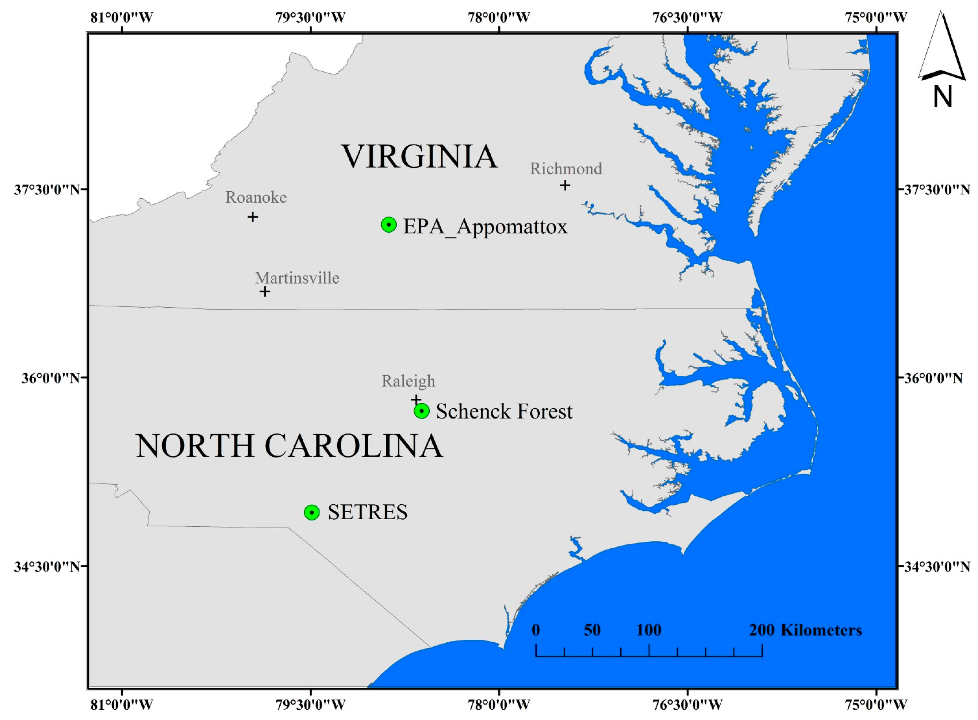
The goal of this study was to assess the uncertainty in the creation of a fine-resolution LAI-RM for a 1-km² heterogeneous landscape in southwestern Virginia. Variation of input variables into the modified Beer-Lambert light extinction function was evaluated within the P. taeda forest type. LC classification differences between analysts were also documented and integrated with the in situ variation to produce an additive error distribution.

Study Area

The 1-km² LAI validation site (EPA_Appomattox) is located in Campbell County, Virginia (37.219° N, −78.879° W) approximately 15.5 km SSW of Appomattox, Virginia (Figure 1). This Upper Piedmont region has a range in elevation from 165 m to 215 m above mean sea level. The area is a mixture of rural agricultural fields and managed and unmanaged forest stands. The MeadWestvaco Corporation, a supporter of the Sustainable Forestry Initiative, permitted sampling access to the US EPA for LAI research on 505 hectares in 2002. LC percentages within the 1-km² area include: (1) deciduous (i.e., HDWD) (30.8%); (2) coniferous (i.e., PINE) (Total—31.9% (unthinned—25.6%, thinned—6.3%)); and (3) other vegetation (i.e., OV) (Total—37.2% (agriculture—6.0%, harvested—31.2%)). Annual precipitation (2002) recorded at Appomattox, Virginia was 1045 mm, with an average temperature of 13.9°C. The dominant soil types consist of very deep, well-drained, moderately permeable soils (Georgville and Tatum loams) on 2%–15% slopes.

Coniferous and deciduous forest stand types dominated the forest composition on the MeadWestvaco tract (EPA_Appomattox). The primary tree species across the entire site was planted P. taeda with upland deciduous oak (Quercus spp.) comprising the deciduous component. Within the coniferous forest type, unthinned P. taeda planted in 1983 with a 25-year site index value of 18.9, reached economic maturity in 2003 and was subsequently harvested. Stocking values, expressed as trees per hectare (TPH), were 1247 TPH for the dominant-codominant crown class and 3790 TPH for all trees comprising the understory (suppressed). The average diameter at breast height (DBH) was 19.4 cm. The average height of the dominant-codominant crown class was 15.9 m. The conifer stand supported a basal area (BA) per hectare of 36.7 m², with BA defined as the cross-sectional area of a tree at 1.4 m above the tree base per unit area. The crown closure, estimated via a vertical projection, was 71% for this forest type.

The other P. taeda forest stand was planted in 1982 and thinned in early 2002. Prior to thinning, the site was stocked at 1400 TPH with a basal area per hectare of 28.9 m². The mechanical thinning operation reduced the basal area and trees per hectare to 11.5 m² and 282 TPH, respectively, a 60.2% reduction in biomass. The average height and dbh for this stand was 17.1 m and 23.2 cm, respectively. The 25-year site index (SI = 16.2) was lower than that found on the unthinned conifer site (SI = 18.9).

The deciduous component of the Appomattox validation site was primarily northern red oak (Q. rubra), white oak (Q. alba), and chestnut oak (Q. prinus). The average height and dbh for the dominant-codominant crown class was 22.2 m and 26.8 cm, respectively. Stocking at the dominant-codominant crown class was 249 TPH, with a basal area of 22.9 m² per hectare.

Figure 1. LAI study site locations include the 1-km² validation site (EPA_Appomattox) and the two sites where modified Beer-Lambert light extinction model variables were assessed (Schenck Forest, SETRES).

Figure 1. LAI study site locations include the 1-km² validation site (EPA_Appomattox) and the two sites where modified Beer-Lambert light extinction model variables were assessed (Schenck Forest, SETRES).

2. Methods

Uncertainty was assessed for elements within the process of creating a 1-km² LAI-RM (23 May 2002) used in the validation of a moderate resolution LAI pixel located at the EPA_Appomattox site (37.219°N, −78.879°W). First, measurement uncertainty and natural variability were estimated from the indirect in situ optical LAI estimation technique combining measurements from the TRAC optical sensor and DHP in P. taeda forest stands. Parameters assessed within the TRAC-DHP method included the element clumping index (Ω_E) derived from the TRAC instrument, the effective leaf area index (L_e) measured with DHP, the needle-to-shoot area index (λ_E) measured in the field and in the laboratory, and the woody-to-total area ratio (α) also measured in the field. Within the deciduous component, the only accounted for uncertainty was the associated natural variability of TRAC-DHP derived LAI. With this information, uncertainty ranges were calculated for each LC class found within the 1-km² validation cell. LC classes constrained to this analysis were defined as: Deciduous Forest, Coniferous Forest (thinned and unthinned), and Other Vegetation (agriculture and harvested). Finally, inter-analyst classification variability based on training signature selection was assessed to determine the range of LC proportions over the area of interest. Contributed variability from the indirect in situ optical measurements and the LC classifications were combined to arrive at a mean LAI value with associated variance for the 1-km² LAI-RM.

2.1. Modified Beer-Lambert Input Uncertainty (Ω_E—TRAC, L_e—DHP, λ_E and α—Field and Laboratory)

Inputs to the modified Beer-Lambert light extinction function were investigated at two locations to assess uncertainty. Element clumping (Ω_E) and effective leaf area (L_e) variability within both TRAC and DHP measurements were made primarily at the Schenck Forest (35.8176° N, 78.7197° W) located in western Raleigh, North Carolina and managed by the North Carolina State University School of Forestry (Figure 1). This site is primarily even-aged P. taeda planted in 1938. Variation in needle-to-shoot and woody-to-total ratios was made at the Southeast Tree Research and Education Site (SETRES), a site that is part of a P. taeda long-term nutritional study established by the North Carolina State Forest Nutritional Cooperative. SETRES is located in the Sandhills Ecosystem of Scotland County, North Carolina (34.917° N, 79.500° W) (Figure 1).

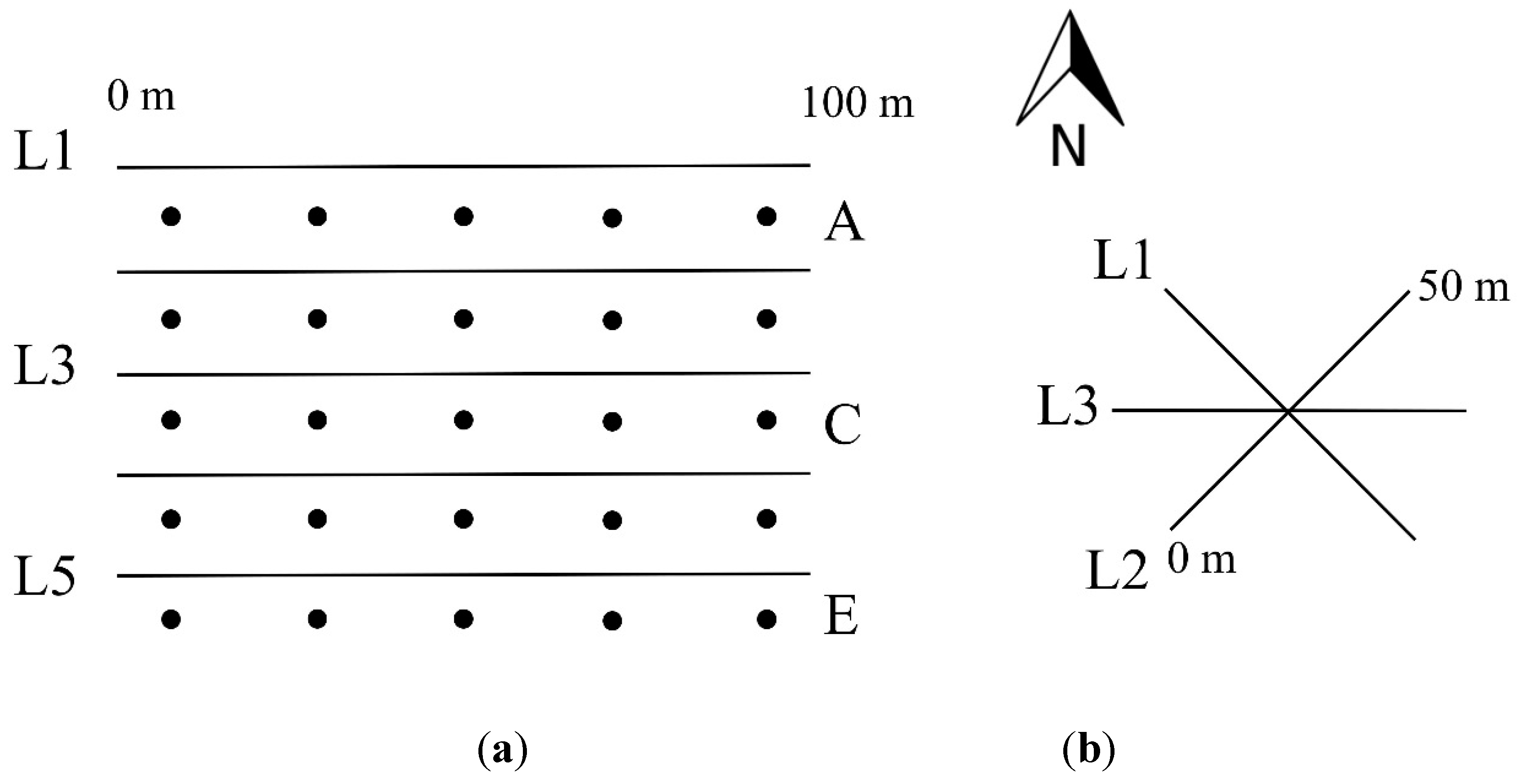
2.1.1. Sampling Design: Optical Instrument Descriptions and Plot Design

The TRAC sunfleck-profiling instrument consists of three quantum photosynthetically active radiation (PAR) (400–700 nm) sensors (LI-COR, Lincoln, NE, Model LI-190SB)—two uplooking and one downlooking—mounted on a wand with a built-in data logger [28]. The instrument is hand-carried in direct sun conditions under the canopy along a linear transect at a constant speed of 0.3 m/s. The instrument records the downwelling solar photosynthetic photon flux density (PPFD) from one of the uplooking sensors in units of μmol/m²/s at a sampling frequency of 32 Hz. The data logger records light-dark transitions as the direct solar beam is alternately transmitted and eclipsed by canopy elements. TRAC data are processed by TRACWin software [28] to yield the element clumping index (Ω_E) from the deviation of the measured gap-size distribution from that of randomly distributed foliage [2]. TRAC data quality is influenced by solar zenith and azimuth. Optimal results are achieved with a solar zenith angle θ between 30° and 60°. As θ approaches the horizon (θ > 60°), the relationship between LAI and light extinction becomes increasingly nonlinear. Similarly, best results are attained when TRAC sampling is conducted with a solar azimuth perpendicular to the transect azimuth. Sky condition is also a significant factor for TRAC measurements. Clear blue sky with unobstructed sun is optimal. Overcast conditions are unsuitable; the methodology requires distinct sunflecks and shadows.

DHP measurements were made with a Nikon CoolPix 995 digital camera with a Nikon FC-E8 fish-eye converter in diffuse light conditions [41]. Gap Light Analyzer (GLA) software (Simon Fraser University, Burnaby, British Columbia, Canada) was used to process the DHP imagery. After downloading the images, an analyst-derived threshold value was determined between sky (white pixels) and no-sky (black pixels). Gap fraction was determined at 57.3° by mapping L_e values at the 4th ring (0°–60°) and the 5th ring (0°–75°). Solving for L_e from the modified Beer-Lambert light extinction function results in:

L_e = ln P(θ) [−2cos(θ)]

(4)

where P(θ) is the gap fraction at zenith angle θ.

The primary sampling unit was the quadrant, a 100 m × 100 m grid with five 100-m east-west TRAC sampling transects, separated 20-m apart. Interspersed between the TRAC transects were five DHP transects, with 20-m separation between each DHP plot location. The secondary sampling unit was three intersecting 50 m or 100 m transects at 45°, 90° and 225° (Figure 2). TRAC measurements were made along transects closest to perpendicular to the solar azimuth at sampling time between the solar zenith angles of 30° and 60°. DHP measurements were located along each transect at the 10 m, 50 m and 90 m mark and were made during diffuse light conditions (i.e., dawn or dusk).

Figure 2. (a) TRAC-DHP 100-m quadrant. Five 100-m TRAC lines separated by 20 m. DHP sample points interspersed 20-m apart between TRAC lines. (b) Sub-plots with three TRAC lines (50 m and 100 m) at 45°, 90°and 225° azimuths.

Figure 2. (a) TRAC-DHP 100-m quadrant. Five 100-m TRAC lines separated by 20 m. DHP sample points interspersed 20-m apart between TRAC lines. (b) Sub-plots with three TRAC lines (50 m and 100 m) at 45°, 90°and 225° azimuths.

2.1.2. Modified Beer-Lambert Uncertainty

Effective LAI (L_e), measured by DHP, was tested for two types of variability: inter-operator and light-regime differences. Inter-operator differences between 10 analysts in the selection of appropriate threshold values delineating photosynthetic from non-photosynthetic canopy elements were tested over 30 DHP images acquired in Oregon. Seven of the analysts were participants in a study investigating stream solar exposure in Corvallis, Oregon, while the other three analysts were associated with a LAI research project based in Research Triangle Park, North Carolina [42]. A single factor analysis of variance (ANOVA) (α = 0.05) was run to test for thresholding differences between analysts. Light regime differences were tested at the Schenck Forest with five sequential images acquired by one operator between 7:54 pm and 8:38 pm on 6 August 2004. These images were acquired to establish the L_e variability attributed to decreasing diffuse light conditions. DHP images were processed by one analyst with GLA software to arrive at L_e.

Clumping Index (Ω_E) acquired by TRAC was tested for five elements of uncertainty: (1) solar zenith angle variability, (2) atmospheric variability, (3) intra-operator and (4) inter-operator differences, and (5) Mean Element Width (MEW) variability. Solar Zenith Angle Variability (1), the effect of changes in solar zenith angle on Ω_E, was tested at the Schenck Forest site. Multiple TRAC measurements were made between 9:08 am and 10:22 am on 11 August 2004, within a solar zenith angle range from 59.2° to 44.9°. Summer atmospheric conditions vary significantly in the North Carolina and Virginia regions. To test the effects of varying atmospheric conditions (2) on Ω_E, TRAC measurements were made at the Schenck Forest site directly following the passing of a frontal system that brought clear and stable conditions initially then degraded into the typical hazy, hot, and humid environment typifying this area. The frontal system brought heavy rain on 5 August 2004. TRAC measurements were made at approximately 9:00 am for five days beginning the following day and continuing through 11 August 2004. Limiting the measurement period to this particular time allowed for the collection of PPFD to occur within a narrow solar zenith angle range of 60.6°–55.9°. Analysis of the data was made in SAS Release 8 (1999) (SAS Institute Inc., Cary, NC, USA) using the PROC AUTOREG procedure. PROC AUTOREG estimates and forecasts linear regression models for time-series data when the errors are autocorrelated or heteroscedastic. This procedure tests for a linear trend in time. Intra-operator differences (3) were tested by one operator at the Schenck Forest site between the dates of 6 August through 11 August 2004. The operator made back-to-back TRAC collections along a 50-m transect between the hours of 9:00 am and 10:00 am daily with the exception of an afternoon collection (3:00 pm) on 7 August 2004. SZA differences were minimized (Mean = 0.602°, Min = 0.420°; Max = 1.02°; SD = 0.166°). A paired t-test generated from Microsoft Excel statistical analysis module tested Ω_E differences for 13 paired trials. Inter-operator differences (4) were tested between two operators who ran four back-to-back TRAC collections on 11 August 2004 along one 50-m transect Schenck Forest site. These paired dual operator TRAC collections were tested for differences using a paired t-test for two sample means. The primary sampling element within the TRAC algorithm for coniferous species is the shoot and the individual leaf for deciduous species. TRACWin software requires a user defined MEW to determine Ω_E. MEW (5) was varied between 36 mm and 46 mm for P. taeda on the quadrant Q1P in Appomattox for the date 6 March 2002. This date was chosen for MEW analysis due to the limited obstruction from the leafless understory in the TRAC acquisition of PPFD through the dominant-codominant P. taeda overstory.

The needle-to-shoot area ratio (λ_E) was obtained through laboratory analysis of shoot samples [43,44,45]. Three trees in the dominant canopy crown class were randomly selected from two P. taeda sites. Within each tree, four shoot samples were taken from the lower, middle, and upper sections of each crown. Shoots were defined as the combination of the prior and current year needle growth. Therefore, one sampled tree yielded 12 shoot samples. Samples were hydrated and cooled to retain leaf moisture and then transported back to the laboratory for analysis.

The woody-to-total area ratio accounts for the percentage of woody material contributing to the calculation of gap fraction. The woody-to-total area ratio was determined through a combined analysis approach isolating and retrieving the surface area measurement of the main stem area with UTHSCSA ImageTool 3.0, and then analyzing the main canopy with ERDAS Imagine 2014 software using an unsupervised clustering algorithm, the Iterative Self-Organizing Data Analysis Technique (ISODATA) [46]. Four trees were selected from both plots for analysis. Selection criteria included relative isolation of the tree of interest, thus reducing vegetation overlap with neighboring canopies. Lateral images were taken with a Sony Digital Cyber-Shot DSC-S85 at 96-dpi resolution. Images were brought into ImageTool, calibrated, and then the areas of both the main stem and the canopy were computed through on-screen digitization. The main canopy image was clipped and imported as a TIFF (tagged image file format) image into ERDAS Imagine 2014 software and the ISODATA clustering algorithm was used to separate green vegetation from the sky.

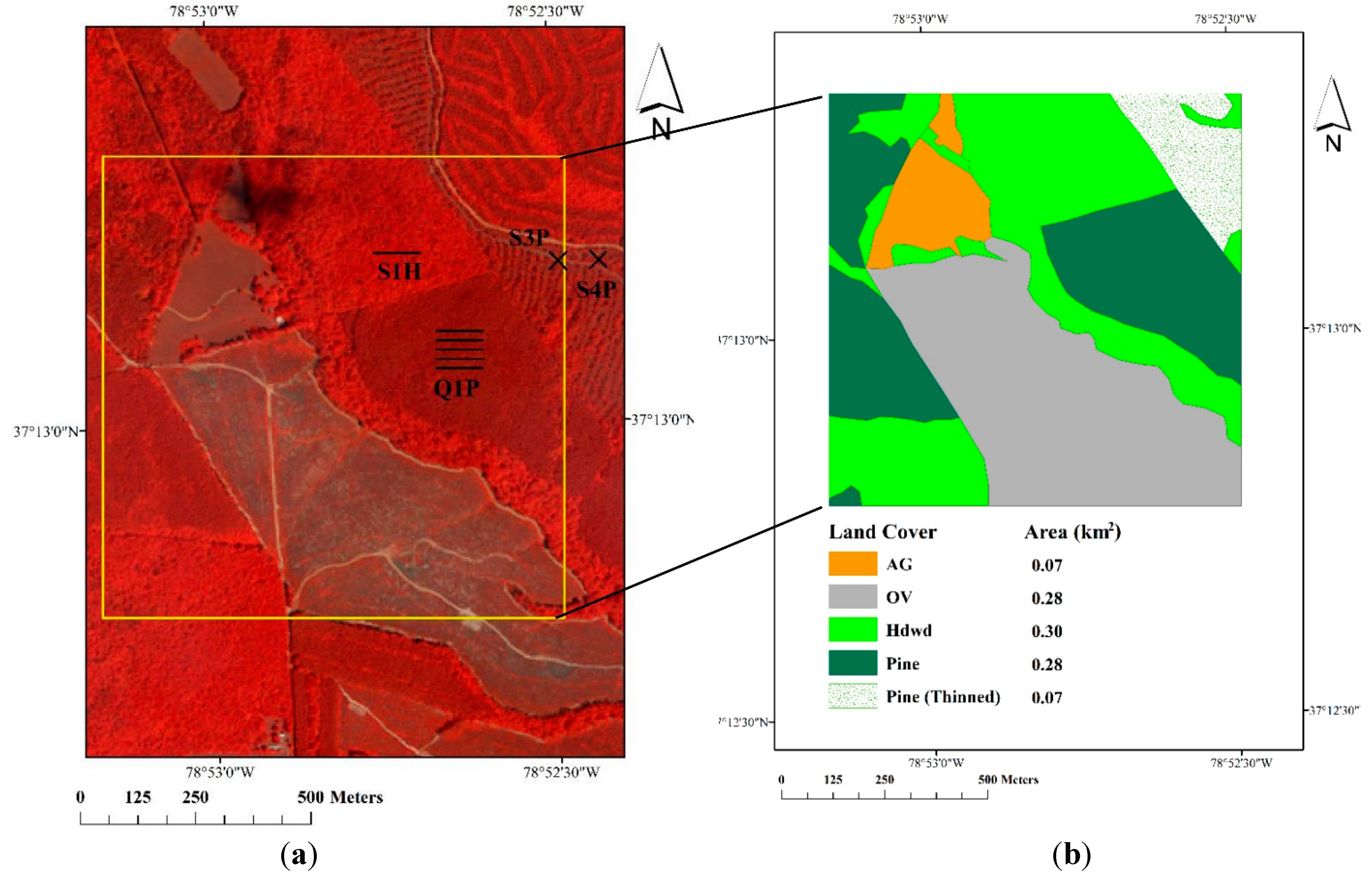
2.2. Land Cover Classification Uncertainty

In a prior study, analyst variation was examined in the LC image classification for a Landsat 7 ETM+ image [29]. This study tested the effect of varying training site selections (location and number) among six analysts performing a supervised classification on a Landsat ETM + image centered on the EPA_Appomattox study site (Path:16, Row: 34; 12 August 2002). We examined the effects of inter-operator variability in their selection of training pixels for the supervised LC classification. In summary, analysts selected training sites via a region growing method where a model pixel is chosen for a particular LC and contiguous pixels are either included or excluded based on the comparative spectral distance to this model pixel. Design constraints maintained other aspects of the classification process constant (i.e., type of classifier, choice of band combinations, etc.) and results indicated that training site selection alone did not provide a predictive measure of classification accuracy. These six supervised classifications were used to identify percent differences in land cover types. These classifications originally included a “mixed forest” LC class. For this study, only the deciduous and coniferous LC classes were included along with other vegetation (agricultural and woodland harvested). The mixed forest class was re-allocated to the other classes by (1) creating a reference classification then (2) reassigning the “mixed forest” pixels by the reference class. This reallocation was necessary because in situ measurements were valid only in homogeneous stand types (i.e., coniferous, deciduous, etc.). Percent LC was then assessed for all six classifications and compared to the reference classification.

2.3. Upscaling Process

At the EPA_Appomattox validation site, one 100-m (S2P) and two 50-m (S3P and S4P) subplots were established in the thinned P. taeda forest stand. Within the unthinned P. taeda, one 100 m × 100 m quadrant (Q1P) was located (Figure 3). Plot locations were randomly selected with the only stipulation being ease of access to a road or open area, a necessary requirement for obtaining outside PPFD readings with the TRAC instrument. Only one transect line of 100 m was established in an east-west direction at the deciduous subplot S1H. TRAC and DHP variables were collected at all sites on 23 May 2002. The clumping index from TRAC (Ω_E) was calculated in 20 m segments. LAI derived from the modified Beer-Lambert light extinction function was calculated for DHP locations in all plots combining the DHP value (L_e) with the average of adjacent 20 m TRAC segment clumping index values.

As mentioned earlier, the validation process for a moderate resolution LAI product involves the creation of a high spatial resolution LAI-RM—which when scaled to the moderate LAI resolution (i.e., > 1 km)—allows for comparison and analysis with the moderate resolution LAI product. In situ LAI values partitioned by LC class are then correlated with spectral values retrieved from high resolution imagery (20–30 m). If regression estimates indicate a reasonable fit (i.e., r² > 0.40), this relationship is applied to the entire image. However, theory and reality diverge when investigating the relationship between LAI and spectral signal, especially with LAI values approaching 3.0 or larger [47]. Linear relationships between increasing vegetation and reflective correspondence do not occur over the entire range of possible values. This effect, an asymptotic increase of vegetation indices to increasing LAI, is termed saturation. The root of the LAI saturation problem with respect to satellite vegetation indices hinges on (1) leaf-level differences (pigments, internal leaf structure, leaf orientation) [47,48,49,50], (2) within-tree crown differences (clumping and woody material contribution to total reflectance) [48,51], and (3) differences in canopy-level parameters such as tree height heterogeneity and the size and number of tree gaps [52,53,54]. The vegetation index saturation issue with respect to increasing vegetation biomass is a function of the near flat response in the red reflectance and the significant positive increase in the NIR reflectance for LAI values exceeding 2.0 in moderate to high vegetative biomass areas [55].

Figure 3. EPA_Appomattox 1-km² validation site. (a) Quadrant (Q1P) and sub-plot distributions (S3P, S4P, S1H) in the vicinity of the validation area (yellow box) are shown. Note: This image is an infrared false color composite of Ikonos imagery collected 24 May 2002 (coniferous—lower reflected IR (dark red); deciduous—lighter reflected IR (light red)) (b) Land cover reference map for 1-km² validation site.

Figure 3. EPA_Appomattox 1-km² validation site. (a) Quadrant (Q1P) and sub-plot distributions (S3P, S4P, S1H) in the vicinity of the validation area (yellow box) are shown. Note: This image is an infrared false color composite of Ikonos imagery collected 24 May 2002 (coniferous—lower reflected IR (dark red); deciduous—lighter reflected IR (light red)) (b) Land cover reference map for 1-km² validation site.

To contend with this saturation issue, we employed an algorithm (i.e., SR LAI) that ingested a Landsat 7 ETM+ derivative band, the vegetation index simple ratio (SR), and accurately predicted managed P. taeda LAI when compared to in situ LAI values (approximately 14% error) [56]. In this study, we used this relationship to predict LAI within the P. taeda component of this site, adjusting the predicted LAI values with our ground-based LAI values. A cloud-free 23 May 2002 image from Landsat 7 ETM+ was acquired from the USGS EarthExplorer repository [57]. This image was clipped to the EPA_Appomattox 1 km² extent and processed for LAI using this SR algorithm [56]. Deciduous LAI was estimated for the 30.8% area represented by this LC class using the mean of the ground-based measurements (n = 3). LAI for the LC class “other vegetation” was segmented into “agriculture” (6% of area) and “harvested” (31.2% of area) and was estimated from prior research. Weighted LAI averages were calculated for each LC class and an overall LAI value with natural variation was determined.

2.4. Uncertainty Analysis

Uncertainty within the in situ data collection (P. taeda only) and the LC classification processes were integrated into the overall LAI value and dispersion calculated for the 1 km² area. This process involved applying in situ variation for the unthinned pine to both the extreme (maximum and minimum) LAI values found in the field. LC classification uncertainty was then applied to the individual LC classes. The resulting maximum and minimum dispersion was then compared to the original statistics.

3. Results

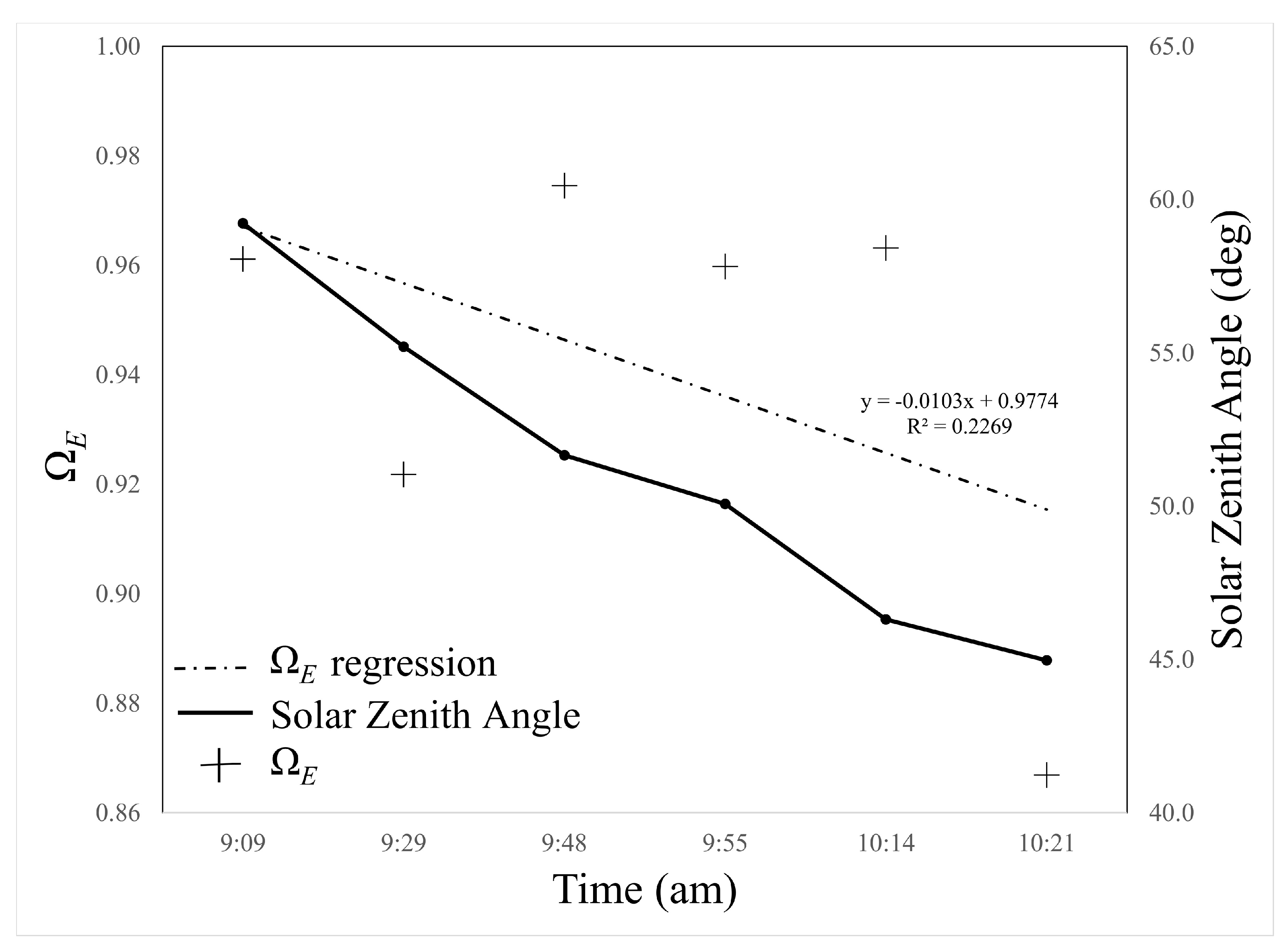
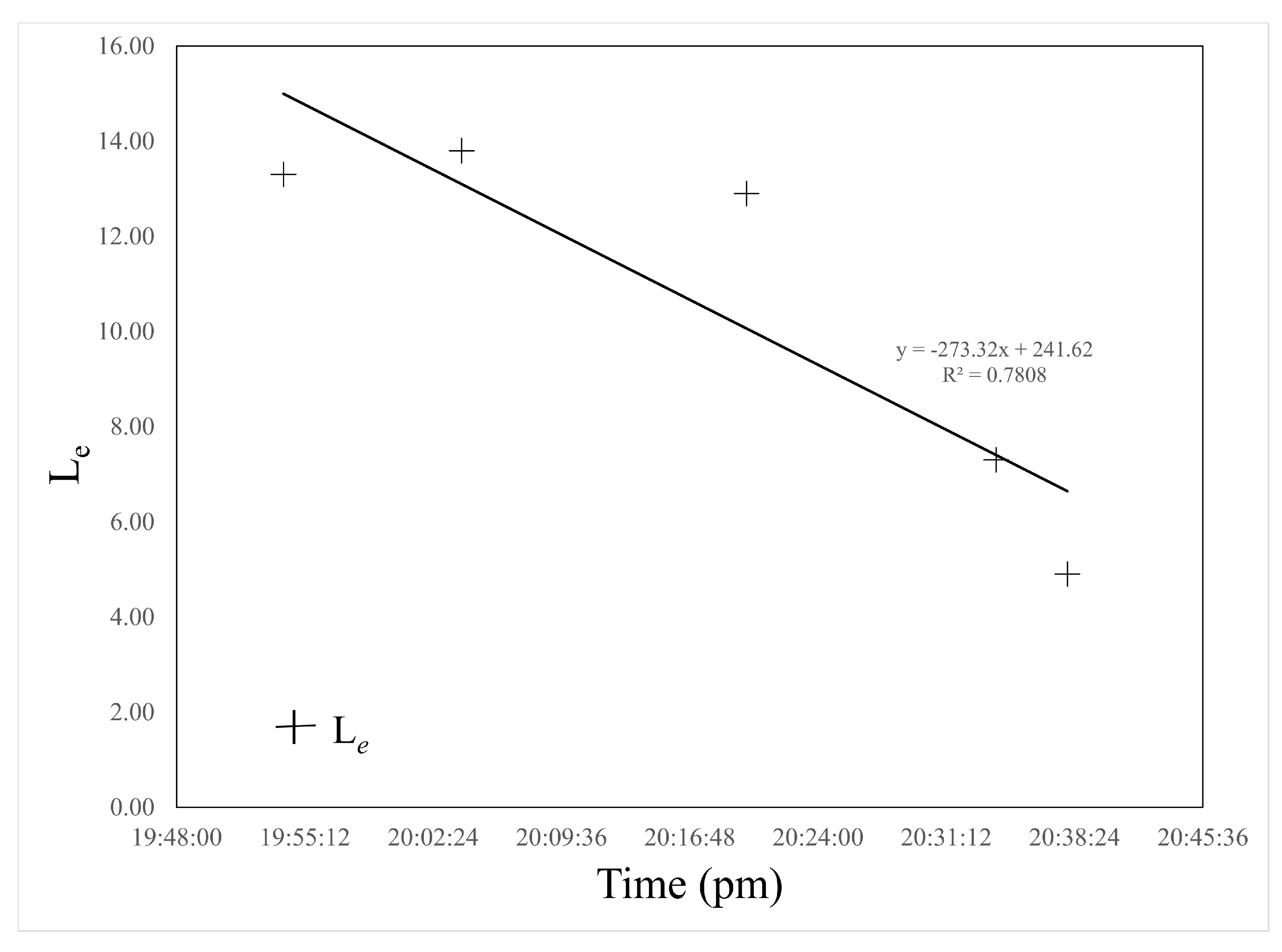
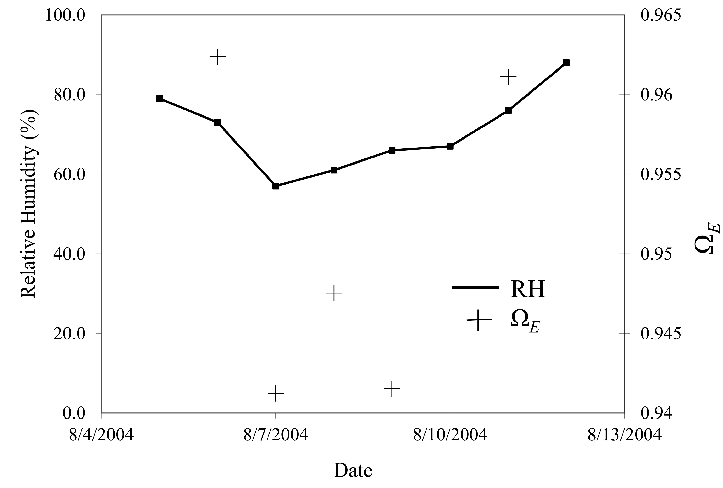
3.1. Modified Beer-Lambert Input Uncertainty (Ω_E—TRAC, L_e—DHP, λ_E and α—Field and Lab)

The effect of atmospheric changes on Ω_E measurements showed a pattern of possible correlation. (Figure 4). High Ω_E was associated with degraded atmospheric conditions after the passing of the cold front, while lower relative humidity was associated with lower Ω_E values. However, the range of Ω_E was exceptionally small (Ω_E = 0.02) implying that the effect of changing atmospheric conditions was relatively insignificant (Figure 4). Results from the regression analysis indicated that there was no significant linear trend effect with respect to time (p = 0.96, t = −0.06, df = 1). Percent variation attributed to this effect was minor (variation = 1.05%).

Inter-operator differences measuring Ω_E were insignificant (p = 0.005, t = 3.18, df = 3), implying no significant differences between the two operators (variation = 0.13%). Intra-operator differences were borderline significant/insignificant (p = 0.056, t = 2.18, df = 12), not warranting a rejection or a non-rejection of the null hypothesis (i.e., Ω_E measured by one operator will return similar values for repeated measurements) (variation = 2.97%). Variation attributed to altering the MEW resulted in a slight variation of 1.17%. Evaluating the linear trends in altering the MEW by 10 mm resulted in nine of the 10 lines exhibiting increasing Ω_E trends with high correlations (r² = 0.68–0.89). Regarding changes in solar zenith angles, no linear trend effect was observed between the measurements of Ω_E (p = 0.44, t = − 0.85, df = 1); however, a slight decrease in Ω_E was observed with changing solar zenith angle assuming the 10:21 am value was not an outlier (variation = 4.31%) (Figure 5). A single factor ANOVA showed no significant differences between 10 analysts in the evaluation of 30 hemispherical images (p = 0.99, F = 0.17, df = 9, variation = 7.43%). Regarding light regime differences in the estimation of Le, a linear trend was found in the estimation of variability ($\overline{x}$ = 2.54, σ = 0.50, r² = 0.78, variation = 19.8%) through a fading light scenario (Figure 6).

The needle-to-shoot area ratio (γ_E) averaged 1.21 (σ = 0.18) over three plots, ranging from a plot mean minimum of 1.00 to a plot mean maximum of 1.32 (variation = 14.88%). Across all three plots, mean γ_E varied by crown position with the top portion of the canopy exhibiting the largest value (γ_E = 1.62). A linear mixed-effects model run in S-PLUS 2000 (Insightful Corp., Seattle, WA) showed that crown position was significant with respect to γ_E controlling for the random tree effect (F = 12.99; df = 2; p < 0.05). Based on an analysis of variance test (F = 1.83; df = 2; p = 0.18), the hypothesis that γ_E means by site were not significantly different was accepted. The woody-to-total ratio also presented a wide range of values over three sites, varying between 0.16 and 0.40. A mean woody-to-total area ratio (α) value of 0.31 (σ = 0.095) was observed for four dominant P. taeda trees (variation = 30.65%). The small crown branches contributed an average of 3.9% to the nonphotosynthetic portion of the trees as analyzed from the lateral image position. Figure 7 provides a summarization of these error components in the modified Beer-Lambert LAI equation for P. taeda.

Figure 4. Atmospheric effects on the element clumping index measured by TRAC. Notice the upward trend coinciding with the lowering of humidity after a cold front passed on 5 August 2004.

Figure 4. Atmospheric effects on the element clumping index measured by TRAC. Notice the upward trend coinciding with the lowering of humidity after a cold front passed on 5 August 2004.

Figure 5. Changing solar zenith angle (degrees) on the element clumping index measured by TRAC. There was a slight positive association between the two variables: as solar zenith angle increased, clumping index increased (r² = 0.23).

Figure 5. Changing solar zenith angle (degrees) on the element clumping index measured by TRAC. There was a slight positive association between the two variables: as solar zenith angle increased, clumping index increased (r² = 0.23).

Figure 6. Fading light effects on estimating the effective LAI (Le) measured by DHP. There was a strong linear trend between L_e and the reduction of light (r² = 0.78).

Figure 6. Fading light effects on estimating the effective LAI (Le) measured by DHP. There was a strong linear trend between L_e and the reduction of light (r² = 0.78).

Figure 7. Error components within the modified Beer-Lambert LAI light extinction function for P. taeda. NV—natural variation.

Figure 7. Error components within the modified Beer-Lambert LAI light extinction function for P. taeda. NV—natural variation.

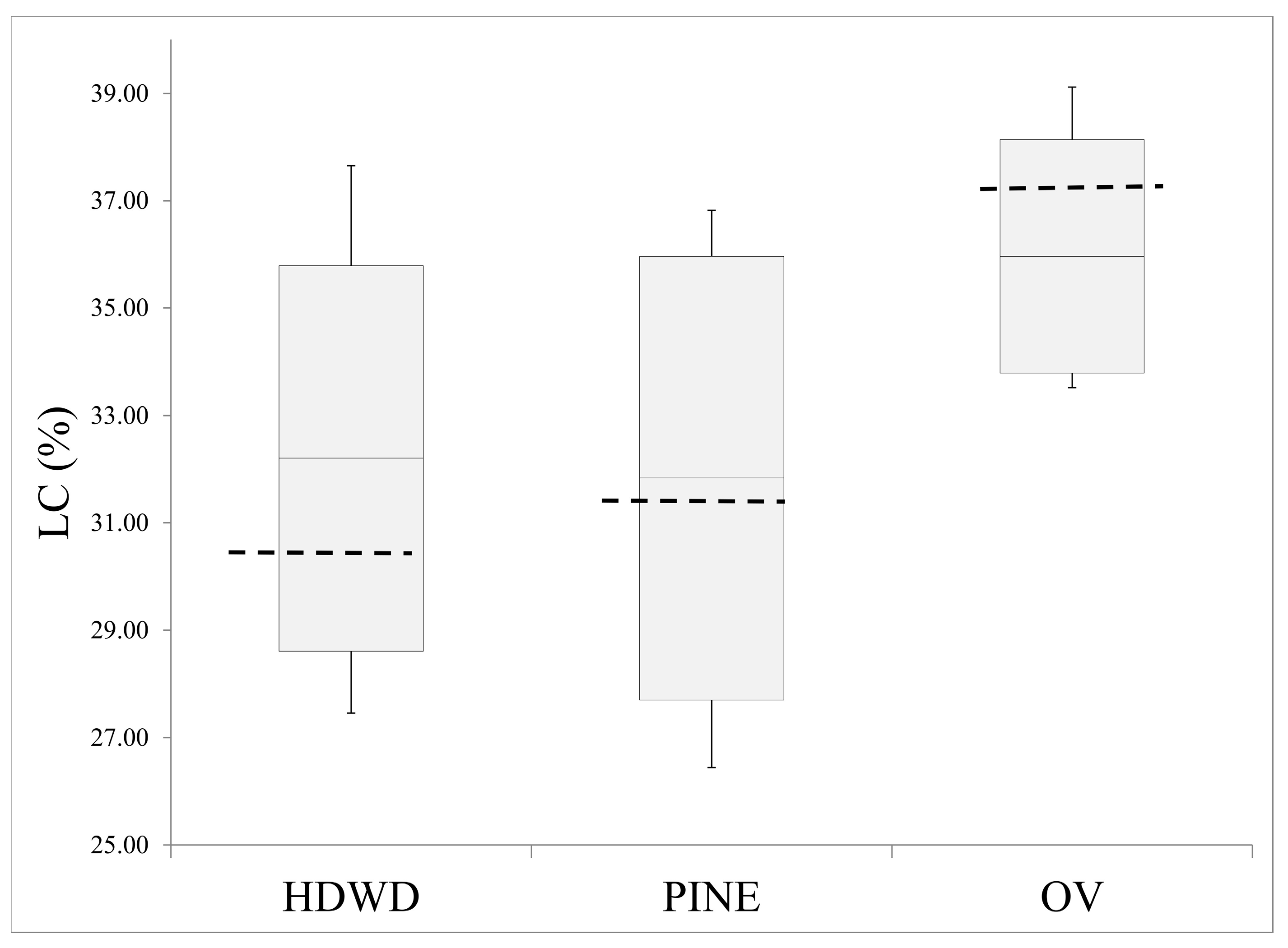
3.2. Land Cover Classification Uncertainty

Highest differences in LC classifications between analysts occurred in the deciduous (LC% range = 10.2) and coniferous (LC% range = 10.4) LC classes (Table 1, Figure 8). There were no significant classification differences between any pair-wise comparisons [29].

Table 1. Analyst variation from classification of the 1-km² area at EPA_Appomattox (OV—Other Vegetation; AG—Agriculture).

LC	Number	Reference (%)	Mean (%)	Min (%)	Max (%)	σ
HDWD	1	30.8	32.2	27.5	37.6	3.6
PINE	2	32.0	31.8	26.4	36.8	4.1
Unthinned	2a	25.6	27.5	22.8	31.4	3.4
Thinned	2b	6.3	4.3	3.5	5.4	0.8
OV	3	37.2	36.0	33.5	39.1	2.2
AG	3a	6.0	5.0	4.7	5.6	0.3
Harvested	3b	31.2	31.0	28.6	33.5	2.0

Table 1. Analyst variation from classification of the 1-km² area at EPA_Appomattox (OV—Other Vegetation; AG—Agriculture).

LC	Number	Reference (%)	Mean (%)	Min (%)	Max (%)	σ
HDWD	1	30.8	32.2	27.5	37.6	3.6
PINE	2	32.0	31.8	26.4	36.8	4.1
Unthinned	2a	25.6	27.5	22.8	31.4	3.4
Thinned	2b	6.3	4.3	3.5	5.4	0.8
OV	3	37.2	36.0	33.5	39.1	2.2
AG	3a	6.0	5.0	4.7	5.6	0.3
Harvested	3b	31.2	31.0	28.6	33.5	2.0

Figure 8. Land cover variability (n = 6) for the classification of 1-km² subset of Landsat 7 ETM+ image, Appomattox, Virginia. Dashed line signifies reference value for each LC class.

Figure 8. Land cover variability (n = 6) for the classification of 1-km² subset of Landsat 7 ETM+ image, Appomattox, Virginia. Dashed line signifies reference value for each LC class.

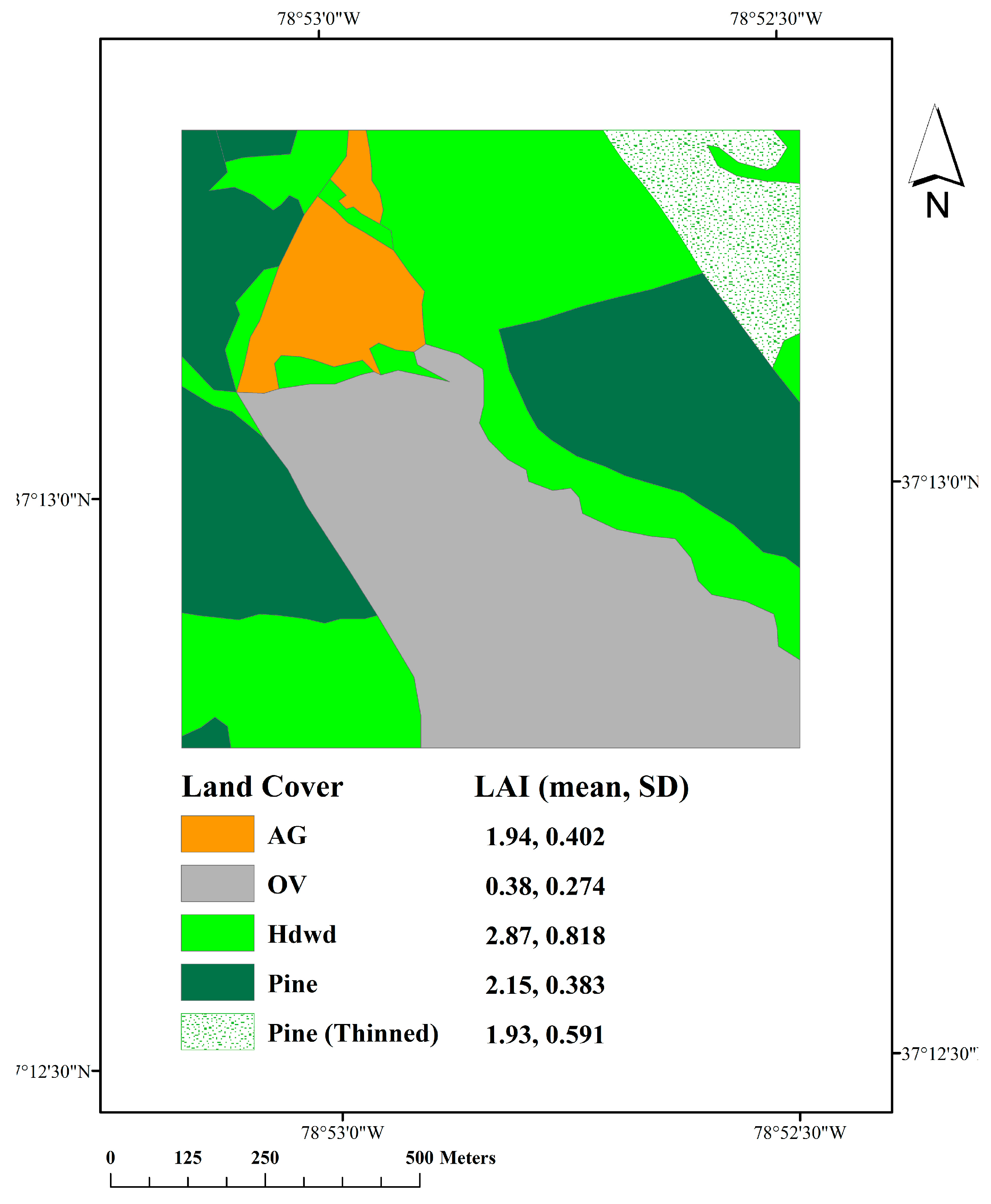
3.3. Upscaling Process

In situ LAI within the unthinned pine stand had a $\overline{x}$ = 1.87 and σ = 0.201. Thinned pine and deciduous in situ LAI was $\overline{x}$ = 0.89 (σ = 0.168) and $\overline{x}$ = 2.87 (σ = 0.818), respectively. There were no significant differences between the means for in situ measured LAI and the LAI derived from the SR ($\overline{x}$ = 1.87, σ = 0.005) algorithm (p = 0.125, df = 20) for the unthinned pine [56]. To adjust between the differences observed between the two means, the SR LAI was increased by 3.8% [56]. The thinned pine component also showed no significant differences between the means of the in situ and SR LAI (p = 0.365, df = 7) [56]. SR LAI was decreased by 14.4%, the difference observed between the two means [56]. The in situ LAI statistics were used for the deciduous LC class ($\overline{x}$ = 2.87, σ = 0.818). For the AG LC class we first identified the crop planted for 2002 in this 670 m2 area as grassland/pasture using the 2002 Crop Data Layer for Virginia. This data layer is produced by the National Agricultural Statistics Service within the United States Department of Agriculture [58]. The SR algorithm produced a distribution ($\overline{x}$ = 1.94, σ = 0.402) similar to that observed [59] for that day of year ($\overline{x}$ = 1.80, σ = 0.572); therefore we retained the SR LAI estimate for this LC. For the OV LC class, there was very little) residual deciduous LAI, so we retained the estimates generated from SR algorithm ($\overline{x}$ = 0.38, σ = 0.274) [56]. Using SR LAI for all LC classes (except for the deciduous LC) yielded mean LAI values ranging from $\overline{x}$ = 0.38 (OV) to $\overline{x}$ = 2.87 (HDWD) (Table 2, Figure 9) [56]. A weighted average per LC class produced a mean of 1.83 and a standard deviation of 0.498 for the 1-km² validation site (Table 2).

Table 2. LAI per LC class as calculated (using SR LAI adjustments [56]) for each pixel within the 1-km² area in Appomattox, Virginia. These values were then area-weighted to arrive at an overall LAI value for the 1-km² validation site (mean LAI = 1.83).

LC	LAI per LC class		Area(%)	LAI per 1 km2
	$\overline{x}$	σ		$\overline{x}$	σ
HDWD	2.87	0.818	29.7	0.85	0.243
PINE Unthinned	2.15	0.383	27.9	0.60	0.107
PINE Thinned	1.93	0.591	7.3	0.14	0.043
OV	0.38	0.274	28.4	0.11	0.078
AG	1.94	0.402	6.7	0.13	0.027
			Total	1.83	0.498

Table 2. LAI per LC class as calculated (using SR LAI adjustments [56]) for each pixel within the 1-km² area in Appomattox, Virginia. These values were then area-weighted to arrive at an overall LAI value for the 1-km² validation site (mean LAI = 1.83).

LC	LAI per LC class		Area(%)	LAI per 1 km2
	$\overline{x}$	σ		$\overline{x}$	σ
HDWD	2.87	0.818	29.7	0.85	0.243
PINE Unthinned	2.15	0.383	27.9	0.60	0.107
PINE Thinned	1.93	0.591	7.3	0.14	0.043
OV	0.38	0.274	28.4	0.11	0.078
AG	1.94	0.402	6.7	0.13	0.027
			Total	1.83	0.498

Figure 9. EPA_Appomattox LAI-RM (23 May 2002)

Figure 9. EPA_Appomattox LAI-RM (23 May 2002)

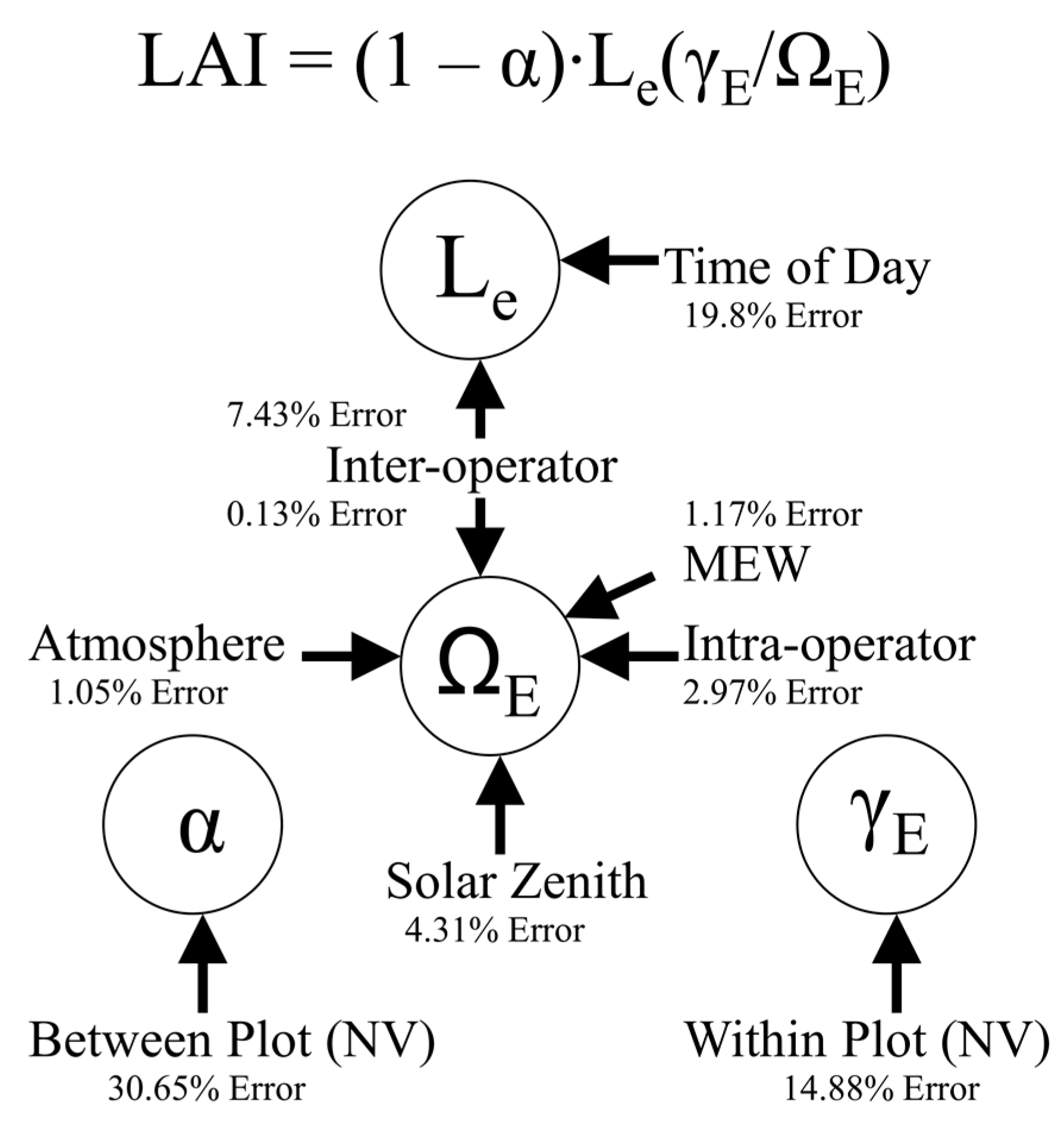
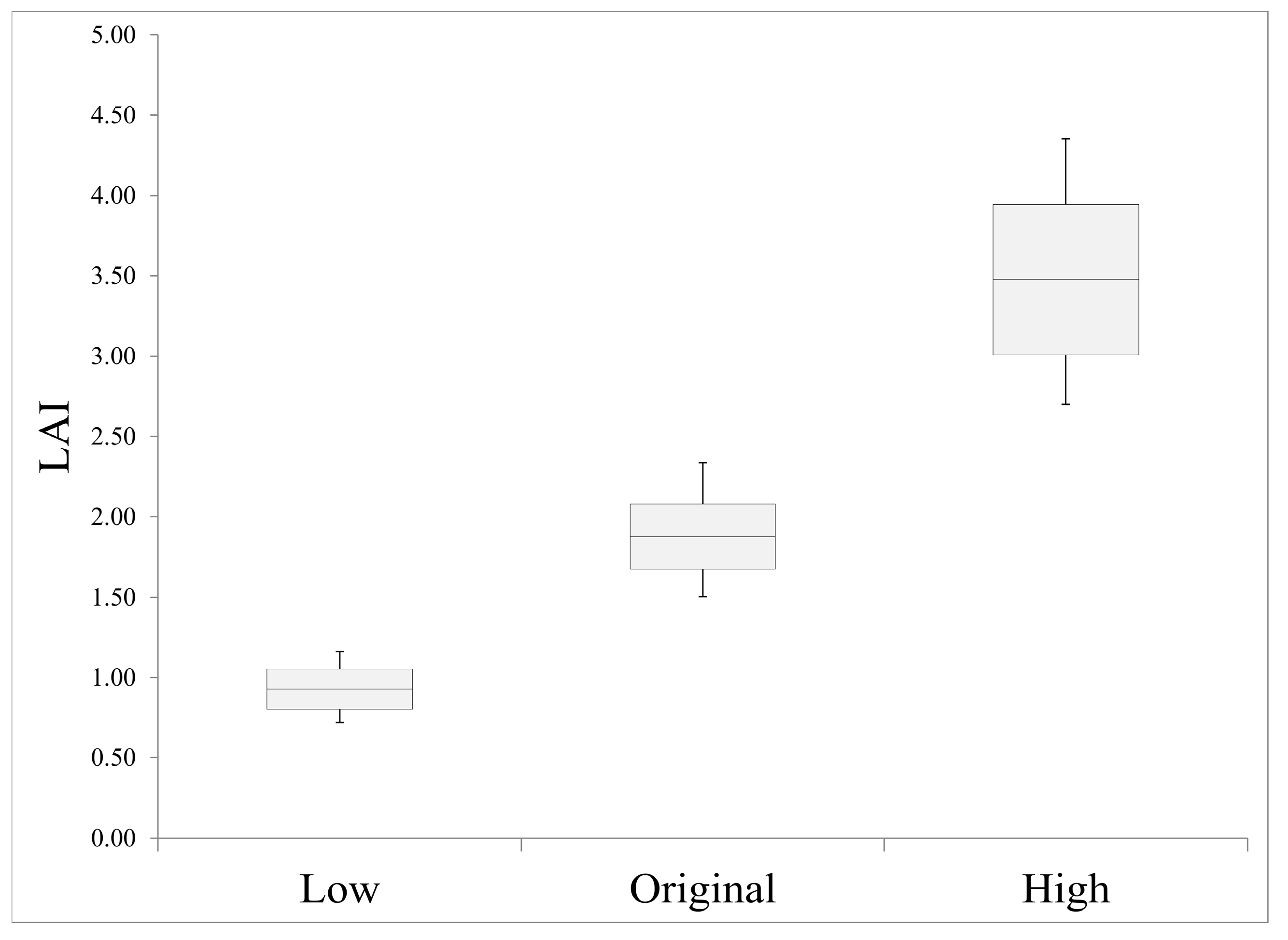
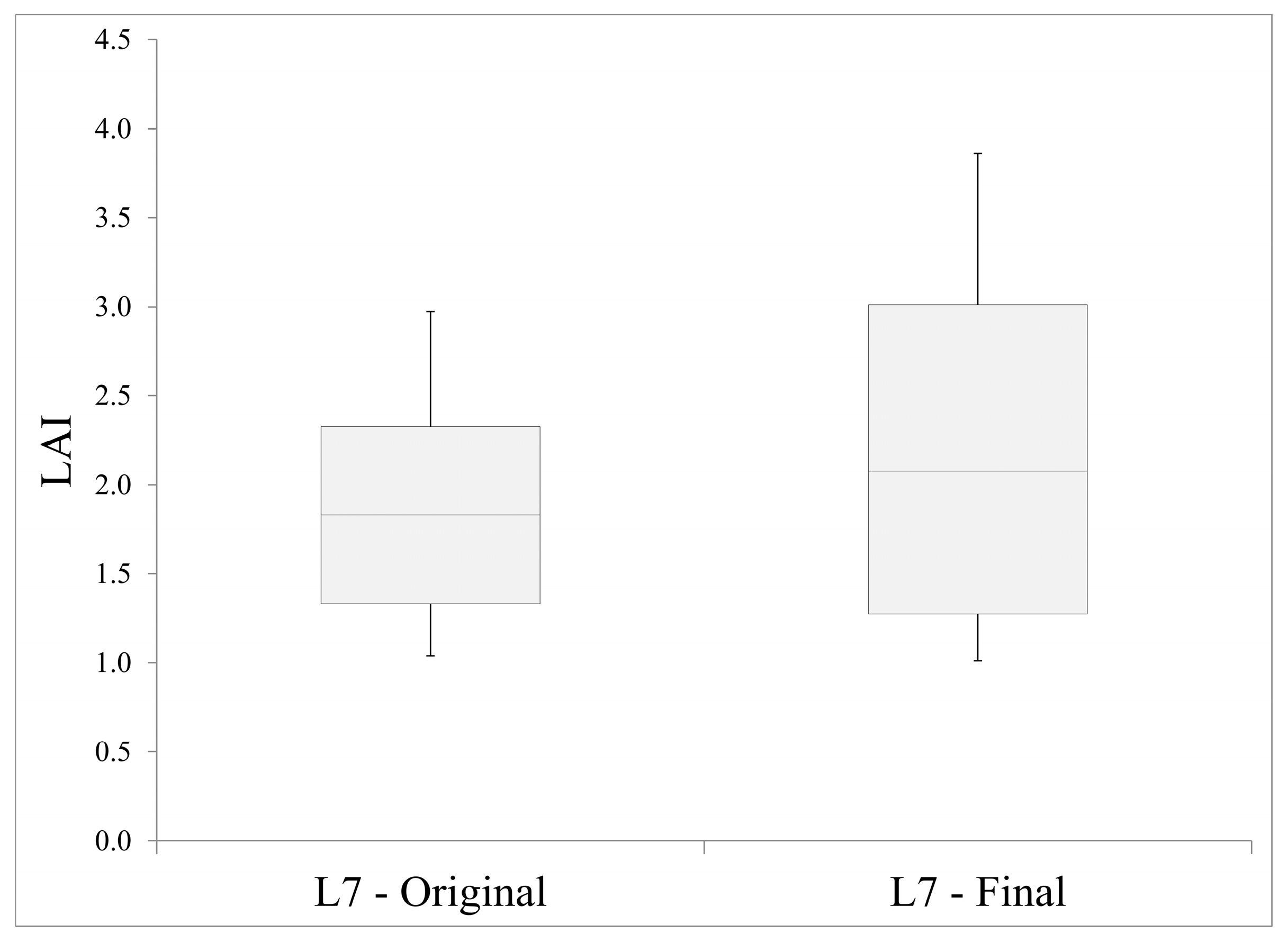
3.4. Uncertainty Analysis

Assuming an additive error model, the application of error components within the modified Beer-Lambert equation for the unthinned pine LC resulted in the following:

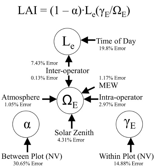
• L_E: 19.86% + 7.4% = 27.2%
• Ω_E: 2.97% + 1.17% + 1.05% + 4.13% = 9.3%
• α: 30.6%
• λ_E: 14.88%

Applying these error values into the modified Beer-Lambert light extinction function over all point locations within the unthinned pine area (n = 21) resulted in a positive 85.3% change in the mean value ($\overline{x}$ = 1.87 to $\overline{x}$ = 3.48) and a negative 50.6% change in the mean value ($\overline{x}$ = 1.87 to $\overline{x}$ = 0.93) (Figure 10).

Figure 10. Unthinned P. taeda LAI integrated with the high and low error values for each modified Beer-Lambert input evaluated at each in situ point (n = 21).

Figure 10. Unthinned P. taeda LAI integrated with the high and low error values for each modified Beer-Lambert input evaluated at each in situ point (n = 21).

Integrating the uncertainty from the unthinned pine LC class along with the variation differences found between classifications (3.36%) resulted in a mean decrease in LAI of 3.4% and a mean increase of 32.2% (Table 3). Averaging all simulated low and high LAI values for each pixel arrives at an overall LAI value with $\overline{x}$ = 2.08 and σ = 0.93 (Figure 11).

Table 3. Overall change in LAI for the 1 km² validation site (Appomattox, Virginia) when integrating variation in the unthinned pine LC class and the uncertainty from differences in LC classifications (L7—Landsat 7 imagery, O—Original LAI, L—Low LAI, H—High LAI).

Stat		Unthinned Pine Only				Unthinned Pine and LC
	L7-O	L7-L	L7-H	% Dec	% Inc	L7-L	L7-H	% Dec	% Inc
Min	1.04	1.01	1.31	-	-	1.01	1.34	-	-
Max	2.97	2.90	3.75	-	-	2.89	3.86	-	-
$\overline{x}$	1.83	1.78	2.34	2.8	27.9	1.77	2.42	3.4	32.2
σ	0.50	0.50	0.59	-	-	0.49	0.59	-	-

Table 3. Overall change in LAI for the 1 km² validation site (Appomattox, Virginia) when integrating variation in the unthinned pine LC class and the uncertainty from differences in LC classifications (L7—Landsat 7 imagery, O—Original LAI, L—Low LAI, H—High LAI).

Stat		Unthinned Pine Only				Unthinned Pine and LC
	L7-O	L7-L	L7-H	% Dec	% Inc	L7-L	L7-H	% Dec	% Inc
Min	1.04	1.01	1.31	-	-	1.01	1.34	-	-
Max	2.97	2.90	3.75	-	-	2.89	3.86	-	-
$\overline{x}$	1.83	1.78	2.34	2.8	27.9	1.77	2.42	3.4	32.2
σ	0.50	0.50	0.59	-	-	0.49	0.59	-	-

Figure 11. Appomattox, Virginia 1 km² area original LAI (L7-Original) comparison with LAI calculated integrating unthinned pine and LC variability (L7-Final)

Figure 11. Appomattox, Virginia 1 km² area original LAI (L7-Original) comparison with LAI calculated integrating unthinned pine and LC variability (L7-Final)

4. Discussion

4.1. Modified Beer-Lambert Input Uncertainty (Ω_E—TRAC, L_e—DHP, λ_E and α—Field and Laboratory)

Differences in the diffuse light intensity had a significant effect on the ability of the analyst to choose the correct threshold for determining gap fraction in the determination of L_e. Decreasing light conditions contribute to the decreasing contrast observable between the conifer shoots and the sky. This light intensity decrease could be responsible for the significantly high variability found within this parameter. Inter-analyst effects on the thresholding of the 30 images showed little difference between analysts. Therefore, the most important factor that determines L_e variability is image quality with respect to resolution and contrast.

The element clumping index (Ω_E) was most affected by changes in the solar zenith angle. The element clumping index increased (i.e., less clumping) with increases in solar zenith angle. This result is consistent with results from other tests in which similar increases in Ω_E corresponded with increases in solar zenith angle for boreal forests [60]. This same pattern observed in P. banksiana and P. mariana suggests that conifer architecture may provide the best explanation for Ω_E change [26]. At nadir, conifer crowns appear solid with small gaps, yet as the sun’s incident radiation approaches the horizon, these small gaps break down into whorls or branches. This disintegration of the canopy architecture into subcomponents would tend to make the canopies less clumped. One other factor, the penumbra effect may, to a lesser extent, distort gap visibility by the optical instrument. At the longer angles, multiple penumbra effects mask small gaps within the canopy, ultimately affecting the gap-size distribution and thus affecting the gap-removal process.

The needle-to-shoot area ratio (γ_E) was by far the most difficult to measure, both in the field and in the laboratory. This parameter was positively correlated with increases in needle biomass over the course of the growing season [26]. Between the sites measured in Virginia and North Carolina, γ_E varied by 24.3%. A 15%–25% variation was recorded in γ_E over one growing season [26]. The mean γ_E value of 1.21 found in this study fell within the range of γ_E values reported in the literature for coniferous forest types. A 1.20–1.40 range in γ_E was recorded for P. banksiana [61,62]. This study only measured γ_E during one time period. It is highly probable that P. taeda γ_E measurements would vary significantly through the growing season due to the accretion and loss of pine needles.

The woody-to-total ratio requires analysis of multiple images and is site and age-class specific. Measurement error involved in the acquisition of α was linked to the difficulty in isolating individual trees. Overlap of adjoining branches would conflate estimates of active photosynthetic area.

4.2. Land Cover Classification Uncertainty

LC differences between multiple analysts (n = 6) were not extensive for identifying the three LC classes (< 11%). However, confusion between LC classes will increase as LC classes increase [29,63]. This has implications in the scaling-up process from higher (20–30 m) spatial resolution to lower spatial resolution (> 250 m). LC differences between analysts produce significant differences in the aggregation process, up to threefold on heterogeneous landscapes [29].

4.3. Upscaling and Uncertainty Analysis Processes

The relationship of in situ P. taeda LAI and LAI predicted from the SR LAI algorithm was highly correlated indicating that the SR algorithm may be useful across managed P. taeda stands [56]. We assumed that error was additive not taking into account any possible covariance. Also, each of the 21 LAI points within the unthinned P. taeda stand were assumed to center within all of the standard deviations of each modified Beer-Lambert variable. This would bias the overall variability higher than the actual. Thus, we have presented here a maximum error or “worst case” scenario (with respect to variability).

5. Conclusions

This research identifies in situ measurement error for LAI and land cover classification variability between analysts, and also characterizes the propagation of these uncertainties in the creation of a 1 km² LAI-RM. The site chosen for this research was a highly heterogeneous area, typical of the spatial land cover pattern of the southeastern United States. A number of elements of uncertainty were investigated; however, the list is by no means exhaustive. For example, the needle-to-shoot and woody-to-total ratio uncertainties could be explored with respect to differing methods and timing of collection [64,65]. DHP camera set-up in the field may also add to variation, especially with respect to camera height, plot location, and sampling intensity. In deciduous forest stands with a heavy expression of understory, how much of that understory canopy influences the overall effective leaf area is also a question of interest. Also, within the LC classification process, there were interpreter differences that were not investigated including the manual editing that is usually implemented at the end of the classification process. Given that only the supervised classification process was used, it is understood that variability sources will increase with the level of complexity in the classification process (i.e., hybrid classifications). Reallocating the mixed forest class into either deciduous or coniferous classes may also have affected the LC classification differences seen in this study. Measuring leaf area in mixed forest stands is in itself problematic in that modified Beer-Lambert light extinction model input values are different for both deciduous and coniferous forest types.

Assessing the sensitivity of the four modified Beer-Lambert light extinction model variables, beyond the variance measured, the behavior of each variable on overall LAI is also dependent on the position within the equation and whether the range is less than 1 (i.e., Ω_E). As an example, even though the woody-to-total ratio (α) variance was twice that of the needle-to-shoot ratio (γ_E), the γ_E had more impact (20.2% larger increase) on overall LAI when we assumed an increase of 25% in variability for both values. Comparing the effective LAI (L_e) and the element clumping index (Ω_E), L_e showed a 5% larger change in overall LAI when we assumed an increase of 25% in variability for both of these values.

Looking at these variables independently, in the measurement of L_e most of the variation was associated with the time of day the images were acquired. Small canopy gaps became less discernable as the light decreased. Also, intra- and inter-operator variance was small in comparison to the time element source. The variability associated with Ω_E was small in comparison to L_e. Assessing the error associated with γ_E is more problematic in that it is the most time consuming and labor intensive measurement of the four variables. LC classification differences were minor in this study. However, the analysts classified a relatively small region leading to tighter training statistics for area-specific cover types. More variability would be expected with increasing the area of the region classified.

Finally, accounting only for uncertainty within the coniferous class, which represented over 1/3 of the total LC, had an impact of almost doubling the variability over the entire 1 km² validation area. Conflating the uncertainties from the other LC classes would add to our understanding of the LAI-RM comparison to global/regional moderate resolution LAI products.

References

1. Chen, J.M. Optically-based methods for measuring seasonal variation of leaf area index in boreal conifer stands. Agr. Forest Meteorol. 2006, 80, 135–163. [Google Scholar] [CrossRef]
2. Morisette, J.T.; Baret, F.; Privette, J.L.; Myneni, R.B.; Nickeson, J.; Garrigues, S.; Shabanov, N.; Weiss, M.; Fernandes, R.; Leblanc, S.; et al. Validation of global moderate-resolution LAI products: A framework proposed within the CEOS land product validation subgroup. IEEE Trans. Geosci. Remote Sens. 2006, 44, 1804–1817. [Google Scholar] [CrossRef]
3. Foody, G.M. Estimation of sub-pixel land cover composition in the presence of untrained classes. Comput. Geosci. 2000, 26, 469–478. [Google Scholar] [CrossRef]
4. Huang, D.; Yang, W.; Tan, B.; Rautiainen, M.; Zhang, P.; Hu, J.; Shabanov, N.; Linder, S.; Knyazikhin, Y.; Myneni, R.B. The importance of measurement error for deriving accurate reference leaf area index maps and validation of the MODIS LAI product. IEEE Trans. Geosci. Remote Sens. 2006, 44, 1866–1871. [Google Scholar] [CrossRef]
5. Abbaspour, R.A.; Delavar, M.R.; Batouli, R. The issue of uncertainty propagation in spatial decision making. In Proceedings of the 9th Scandinavian Research Conference on Geographical Information Science, Espoo, Finland, 4–6 June 2003; pp. 57–65.
6. Geographic Information Technologies in Society, NCGIA Core Curriculum GIScience. Available online: http://www.ncgia.ucsb.edu/giscc/units/u098/u098.html (accessed on 27 August 2014).
7. Hunter, G.J.; Goodchild, M.F. Modelling the uncertainty of slope and aspect estimates derived from spatial databases. Geogr. Anal. 1997, 29, 35–49. [Google Scholar] [CrossRef]
8. Sampson, D.A.; Albaugh, T.J.; Johnsen, K.H.; Allen, H.L.; Zarnoch, S.J. Monthly leaf area index estimates from point-in-time measurements and needle phenology for Pinus taeda. Can. J. Forest Res. 2003, 33, 2477–2490. [Google Scholar] [CrossRef]
9. Aerts, J.C.J.H.; Goodchild, M.F.; Huevelink, G.B.M. Accounting for spatial uncertainty in optimization with spatial decision support systems. Trans. GIS 2003, 7, 211–230. [Google Scholar] [CrossRef]
10. Maier, C.A.; Johnsen, K.H.; Butnor, J.; Kress, L.W.; Anderson, P.H. Branch growth and gas exchange in 13-year-old loblolly pine (Pinus taeda) trees in response to elevated carbon dioxide concentration and fertilization. Tree Physiol. 2002, 22, 1093–1106. [Google Scholar] [CrossRef] [PubMed]
11. Dougherty, P.M.; Hennessey, T.C.; Zarnoch, S.J.; Stenberg, P.T.; Holeman, R.T.; Wittwer, R.F. Effects of stand development and weather on monthly leaf biomass dynamics of a loblolly pine (Pinus taeda L.) stand. Forest Ecol. Manag. 1995, 72, 213–227. [Google Scholar] [CrossRef]
12. Herbert, M.T.; Jack, S.B. Leaf area index and site water balance of loblolly pine (Pinus taeda L.) across a precipitation gradient in East Texas. Forest Ecol. Manag. 1998, 105, 273–282. [Google Scholar] [CrossRef]
13. Vose, J.M. Patterns of leaf area distribution within crowns of nitrogen- and phosphorus-fertilized loblolly pine trees. Forest Sci. 1988, 34, 564–573. [Google Scholar]
14. Sword, M.A.; Chambers, J.L.; Tang, Z.; Dean, T.J.; Goelz, J.C. Long-term Trends in Loblolly Pine Productivity and Stand Characteristics in Response to Stand Density and Fertilization in the Western Gulf Region. Available online: http://www.treesearch.fs.fed.us/pubs/viewpub.jsp?index=3111 (accessed on 4 September 2014).
15. Teskey, R.O.; Bongarten, B.C.; Cregg, B.M.; Douherty, P.M.; Hennessey, T.C. Physiology and genetics of tree growth response to moisture and temperature stress: An examination of the characteristics of Loblolly pine (Pinus taeda L.). Tree Physiol. 1987, 3, 41–61. [Google Scholar] [CrossRef] [PubMed]
16. Vose, J.; Allen, H.L. Leaf area, stemwood growth, and nutrition relationships in loblolly pine. Forest Sci. 1988, 34, 547–563. [Google Scholar]
17. Colbert, S.R.; Jokela, E.J.; Neary, D.G. Effects of annual fertilization and sustained weed control on dry matter partitioning, leaf area and growth efficiency of juvenile loblolly and slash pine. Forest Sci. 1990, 36, 995–1014. [Google Scholar]
18. Hennessey, T.C.; Dougherty, P.M.; Cregg, B.M.; Wittwer, R.F. Annual variation in needlefall of a loblolly pine stand in relation to climate and stand density. For. Ecol. Manag. 1992, 51, 329–338. [Google Scholar] [CrossRef]
19. Stow, T.K.; Allen, H.L.; Kress, L.W. Ozone impacts on seasonal foliage dynamics of young loblolly pine. Forest. Sci. 1992, 38, 102–119. [Google Scholar]
20. Albaugh, T.J.; Allen, H.L.; Dougherty, P.M.; Kress, L.W.; King, J.S. Leaf area and above- and belowground growth responses of loblolly pine to nutrient and water additions. Forest Sci. 1998, 44, 317–328. [Google Scholar]
21. Yu, S.; Chambers, J.L.; Zhenmin, T.; Barnett, J.P. Crown characteristics of juvenile loblolly pine 6 years after application of thinning and fertilization. Forest Ecol. Manag. 2003, 180, 345–352. [Google Scholar] [CrossRef]
22. Beer, A. Einleitung in Die Hohere Optik; Vieweg und Sohn: Braunschweig, Germany, 1853. [Google Scholar]
23. Jonckheere, I.; Muys, B.; Coppin, P. Allometry and evaluation of in situ optical LAI determination in Scots pine: A case study in Belgium. Tree Physiol. 2005, 25, 723–732. [Google Scholar] [CrossRef]
24. Stenberg, P.; DeLucia, E.H.; Schoettle, A.W.; Smolander, H. Photosynthetic light capture and processing from cell to canopy. In Resource Physiology of Conifers; Smith, W.K., Hinckley, T.M., Eds.; Academic Press: New York, NY, USA, 1995; pp. 3–38. [Google Scholar]
25. Chen, J.M.; Rich, P.M.; Gower, S.T.; Norman, J.M.; Plummer, S. Leaf area index of boreal forests: Theory, techniques, and measurements. J. Geophys. Res. 1997, 102, 429–443. [Google Scholar]
26. Chen, J.M. Optically-based methods for measuring seasonal variation of leaf area index in boreal conifer stands. Agr. Forest Meteorol. 1996, 80, 135–163. [Google Scholar] [CrossRef]
27. Deblonde, G.; Penner, M.; Royer, A. Measuring leaf area index with the LI-COR LAI-2000 in pine stands. Ecology 1994, 75, 1507–1511. [Google Scholar] [CrossRef]
28. Leblanc, S.G.; Chen, J.M.; Kwong, M. Tracing Radiation and Architecture of Canopies; Natural Resources Canada: Ottawa, ON, Canada, 2002. [Google Scholar]
29. Iiames, J.S.; Congalton, R.G.; Lunetta, R.S. Analyst variation associated with landcover image classification of Landsat ETM+ data for the assessment of coarse spatial resolution regional/global landcover products. GISci. Remote Sens. 2013, 50, 604–622. [Google Scholar]
30. Jones, K.; Neale, A.; Wade, T.; Wickham, J.; Cross, C.; Edmonds, C.; Loveland, T.; Nash, M.; Riitters, K.; Smith, E. The consequences of landscape change on ecological resources: An assessment of the US Mid-Atlantic region, 1973–1993. Ecosyst. Health 2001, 7, 229–242. [Google Scholar] [CrossRef]
31. Riitters, K.; Wickham, J.; O’Neill, R.; Jones, K.; Smith, E.; Coulston, J.; Wade, T.; Smith, J. Fragmentation of continental United States forests. Ecosystem 2002, 5, 815–822. [Google Scholar] [CrossRef]
32. Smith, J.; Wickham, J.; Norton, D.; Wade, T.; Jones, K. Utilization of landscape indicators to model pathogen impaired waters. J. Am. Water Resour. Assoc. 2001, 37, 1–10. [Google Scholar] [CrossRef]
33. Wickham, J.; O’Neill, R.; Riitters, K.; Smith, E.; Wade, T.; Jones, K. Geographic targeting of increases in nutrient export due to future urbanization. Ecol. Appl. 2002, 12, 93–106. [Google Scholar] [CrossRef]
34. Powell, R.L.; Matzke, N.; de Souza, C., Jr; Clark, M.; Numata, I.; Hess, L.L.; Roberts, D.A. Sources of error in accuracy assessment of thematic land-cover maps in the Brazilian Amazon. Remote Sens. Environ. 2004, 90, 221–234. [Google Scholar] [CrossRef]
35. Gopal, S.; Woodcock, C. Theory and methods for accuracy assessment of thematic maps using fuzzy sets. Photogramm. Eng. Remote Sens. 1994, 60, 181–188. [Google Scholar]
36. Tran, L.T.; Jarnagin, S.T.; Knight, C.G.; Baskaran, L. Mapping Spatial Accuracy and Estimating Landscape Indicators From Thematic Land Cover Maps Using Fuzzy Set Theory. Available online: http://www.crcnetbase.com/doi/abs/10.1201/9780203497586.ch13 (accessed on 4 September 2014).
37. Foody, G.M.; McCulloch, M.B.; Yates, W.B. Classification of remotely sensed data by an artificial neural network: Issues related to training data characteristics. Photogramm. Eng. Remote Sens. 1995, 61, 391–401. [Google Scholar]
38. Lunetta, R.S.; Congalton, R.G.; Fenstermaker, L.K.; Jensen, J.R.; McGuire, K.C.; Tinney, L.R. Remote sensing and geographical information system data integration: Error sources and research issues. Photogramm. Eng. Remote Sens. 1991, 57, 677–687. [Google Scholar]
39. Stehman, S.V. Statistical rigor and practical utility in thematic map accuracy assessment. Photogramm. Eng. Remote Sens. 2001, 67, 727–734. [Google Scholar]
40. Congalton, R.G.; Green, K. Assessing the Accuracy of Remotely Sensed Data: Principles and Practices, 2nd ed.; CRC Press: Boca Raton, FL, USA, 2009. [Google Scholar]
41. Iiames, J.S.; Congalton, R.G.; Pilant, A.N.; Lewis, T.E. Validation of an integrated estimation of Loblolly pine (Pinus taeda L.) leaf area index (LAI) utilizing two indirect optical methods in the southeastern United States. South. J. Appl. Forest 2008, 32, 101–110. [Google Scholar]
42. Ringold, P.L.; Sickle, J.V.; Rasar, K.; Schacher, J. Use of hemispherical imagery for estimating stream solar exposure. J. Am. Water Resour. Assoc. 2003, 39, 1373–1384. [Google Scholar] [CrossRef]
43. Chen, J.M.; Black, T.A. Foliage area and architecture of plant canopies from sunfleck size distributions. Agric. Forest Meteorol. 1992, 60, 249–266. [Google Scholar] [CrossRef]
44. Chen, J.M.; Black, T.A. Defining leaf area index for non-flat leaves. Plant Cell Environ. 1992, 15, 42l–429. [Google Scholar] [CrossRef]
45. Fassnacht, K.S.; Gower, S.T.; Norman, J.M.; McMurtrie, R.E. A comparison of optical and direct methods for estimating foliage surface area index in forests. Agric. Forest Meteorol. 1994, 71, 183–207. [Google Scholar] [CrossRef]
46. Tou, J.T.; Gonzalez, R.C. Pattern Recognition Principles; Addison-Wesley Pub. Co.: Reading, MA, USA, 1974. [Google Scholar]
47. Baret, F.; Guyot, G. Potentials and limits of vegetation indices for LAI and APAR assessment (absorbed photosynthetically active radiation). Remote Sens. Environ. 1991, 35, 161–173. [Google Scholar] [CrossRef]
48. Williams, D.L. A comparison of spectral reflectance properties at the needle, branch, and canopy level for selected conifer species. Remote Sens. Environ. 1991, 35, 79–93. [Google Scholar] [CrossRef]
49. Bouman, B.A. Accuracy of estimating the leaf area index from vegetative indices derived from crop reflectance characteristics, a simulation study. Int. J. Remote Sens. 1992, 13, 3069–3084. [Google Scholar] [CrossRef]
50. Yoder, B.J.; Waring, R.H. The normalized difference vegetation index of small Douglas-fir canopies with varying chlorophyll concentrations. Remote Sens. Environ. 1994, 49, 81–91. [Google Scholar] [CrossRef]
51. Huemmrich, K.F.; Goward, S.N. Vegetation canopy PAR absorbance and NDVI: An assessment for ten tree species with the SAIL model. Remote Sens. Environ. 1997, 61, 254–269. [Google Scholar] [CrossRef]
52. Cohen, W.B.; Spies, T.A.; Bradshaw, G.A. Semivariograms of digital imagery for analysis of conifer canopy structure. Remote Sens. Environ. 1990, 34, 167–178. [Google Scholar] [CrossRef]
53. Cohen, W.B.; Spies, T.A. Estimating structural attributes of Douglas-fir/western hemlock forest stands from Landsat and SPOT imagery. Remote Sens. Environ. 1992, 4, 1–17. [Google Scholar] [CrossRef]
54. Leblon, B.; Gallant, L.; Grandberg, H. Effects of shadowing types on ground-measured visible and nearinfrared shadow reflectances. Remote Sens. Environ. 1996, 58, 322–328. [Google Scholar] [CrossRef]
55. Gitelson, A.A. Wide dynamic range vegetation index for remote quantification of biophysical characteristics of vegetation. J. Plant Physiol. 2004, 161, 165–173. [Google Scholar] [CrossRef] [PubMed]
56. Flores, F.J.; Allen, H.L.; Cheshire, H.M.; Davis, J.G.; Fuentes, M.; Kelting, D.L. Using multispectral satellite imagery to estimate leaf area and response to silvicultural treatments in loblolly pine stands. Can. J. Forest Res. 2006, 36, 1587–1596. [Google Scholar] [CrossRef]
57. USGS Earth Explorer. Available online: http://earthexplorer.usgs.gov/ (accessed on 27 August 2014).
58. Boryan, C.; Yang, Z.; Mueller, R.; Craig, M. Monitoring US agriculture: The US department of agriculture, national agricultural statistics service, cropland data layer program. Geocarto. Int. 2011, 26, 341–358. [Google Scholar] [CrossRef]
59. Mitchell, R.B.; Moser, L.E.; Moore, K.J.; Redfearn, D.D. Tiller demographics and leaf area index of four perennial pasture grasses. Agron. J. 1998, 90, 47–53. [Google Scholar]
60. Chen, J.M.; Cihlar, J. Quantifying the effect of canopy architecture on optical measurements of leaf area index using two gap size analysis methods. IEEE Trans. Geosci. Remote Sens. 1995, 33, 777–787. [Google Scholar] [CrossRef]
61. Chen, J.M.; Cihlar, J. Retrieving leaf area index of boreal conifer forests using Landsat TM images. Remote Sens. Environ. 1996, 55, 153–162. [Google Scholar] [CrossRef]
62. Gower, S.T.; Kucharik, C.J.; Norman, J.M. Direct and indirect estimation of leaf area index, fAPAR, and net primary production of terrestrial ecosystems. Remote Sens. Environ. 1999, 70, 29–51. [Google Scholar] [CrossRef]
63. Smith, J.H.; Wickham, J.D.; Stehman, S.V.; Yang, L. Impacts of patch size and land-cover heterogeneity on thematic image classification accuracy. Photogramm. Eng. Remote Sens. 2002, 68, 65–70. [Google Scholar]
64. Clawges, R.; Vierling, L.; Calhoon, M.; Toomey, M. Use of a ground-based scanning LIDAR for estimation of biophysical properties of western larch (Larix occidentalis). Int. J. Remote Sens. 2007, 28, 4331–4344. [Google Scholar] [CrossRef]
65. Zhao, F.; Yang, X.; Schull, M.A.; Roman-Colon, M.O.; Yao, T.; Wang, Z.; Zhang, Q.; Jupp, D.L.B.; Lovell, J.L.; Culvenor, D.S.; et al. Measuring effective leaf area index, foliage profile, and stand height in New England forest stands using a full-waveform ground-based LiDAR. Remote Sens. Environ. 2011, 11, 2954–2964. [Google Scholar] [CrossRef]