
Digital Mapping of Soil Properties Using Multivariate Statistical Analysis and ASTER Data in an Arid Region


Abstract
:
1. Introduction
2. Materials and Methods
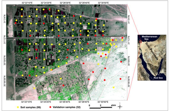
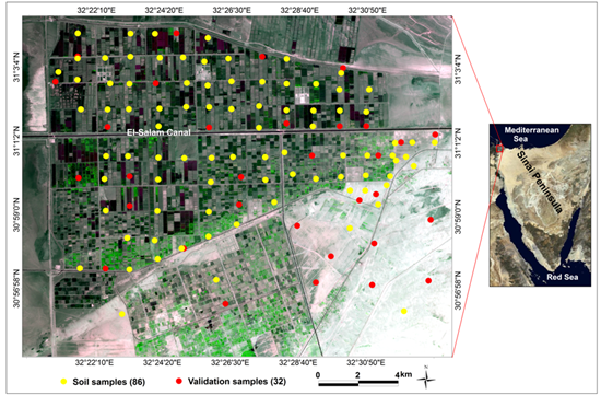
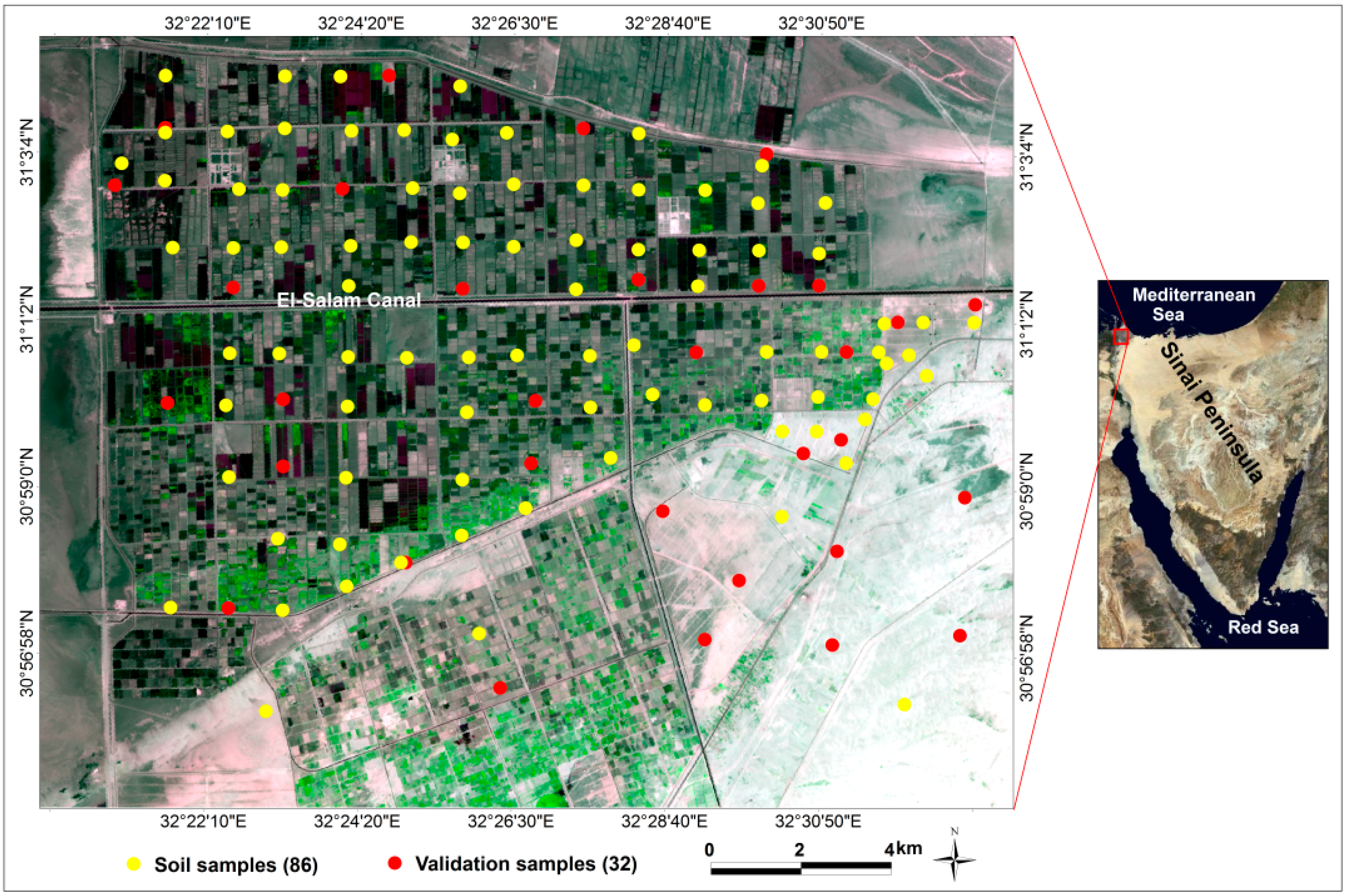
2.1. Study Area

2.2. Soil Sampling and Analysis
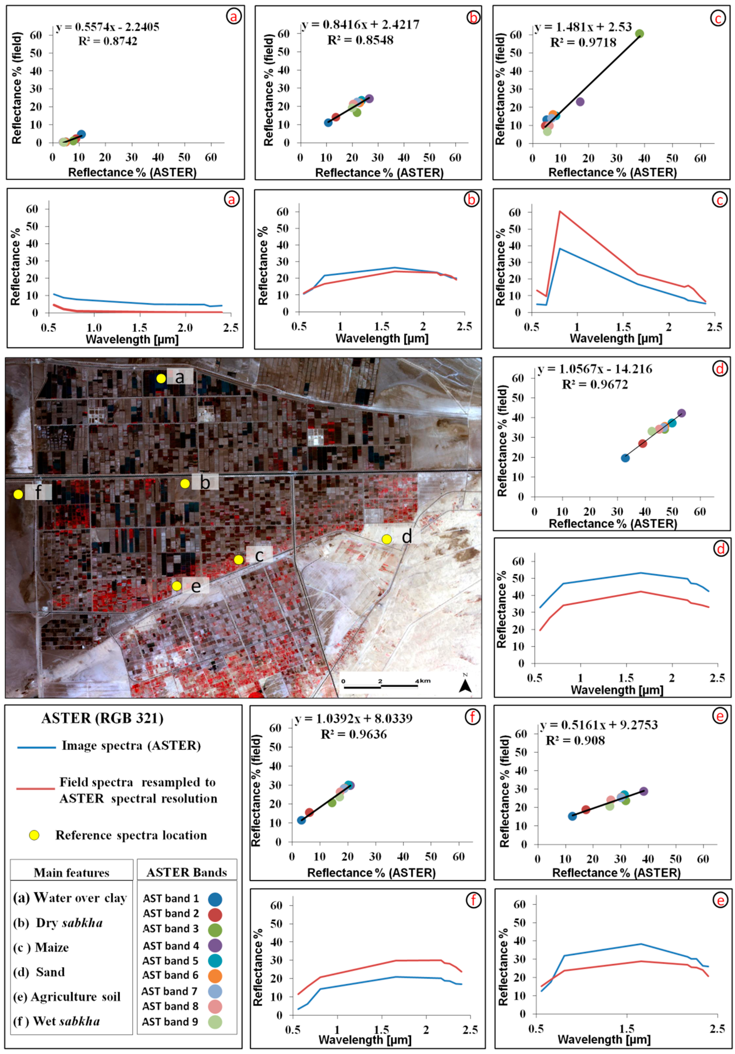
2.3. ASTER Data and Pre-Processing
2.4. Data Analysis
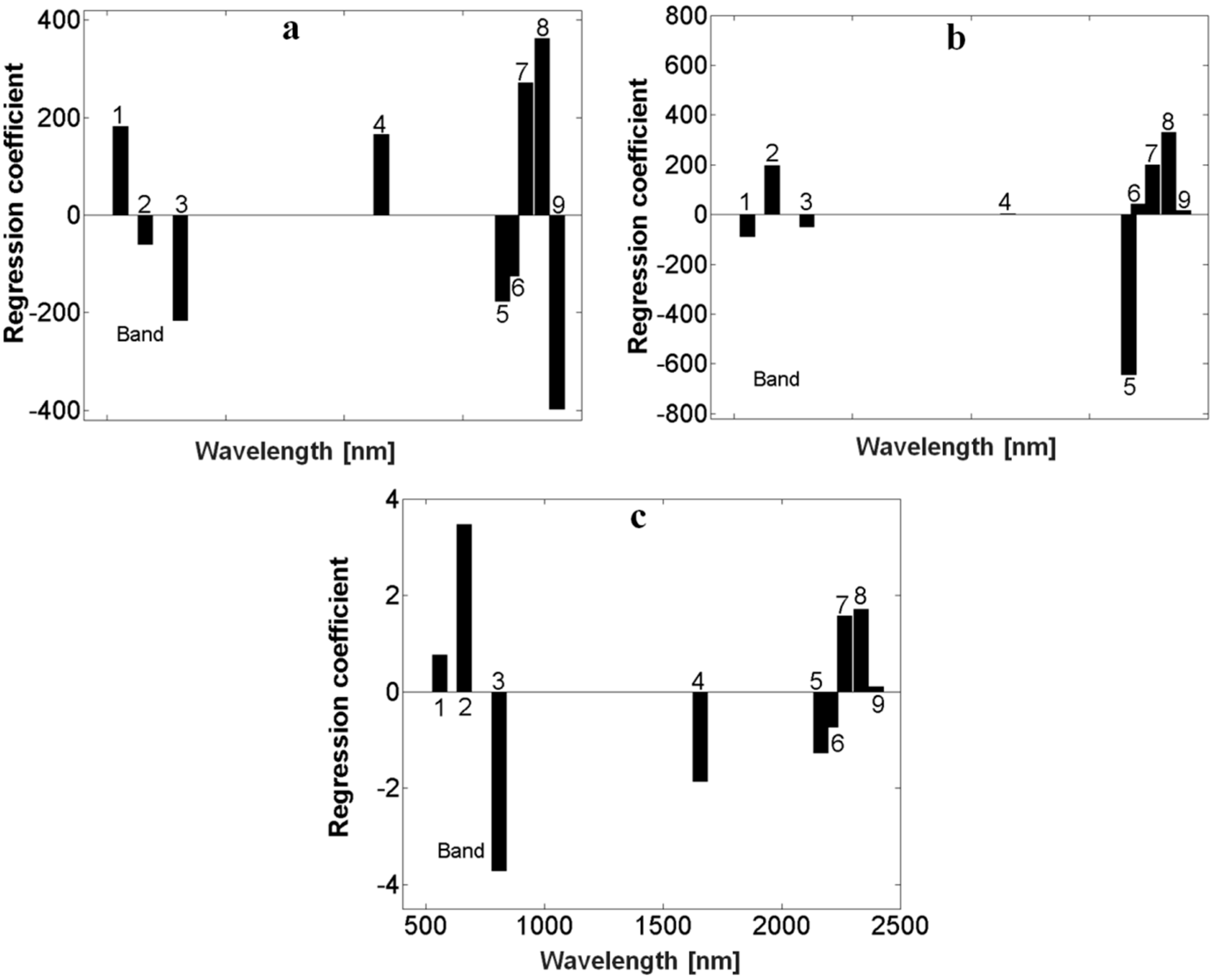
2.4.1. Multivariate Adaptive Regression Splines
2.4.2. Partial Least-Squares Regression
2.4.3. Prediction Accuracy
2.5. Mapping Soil Properties Using ASTER Data

| Soil Units and the Main Features | * Soil Salinity | Water Table (cm) | Land Use/Cover | No. of Soil Samples Modeling/Validation |
|---|---|---|---|---|
| Very deep clay | Very strongly saline | >150 | Salinized soil/bare soil | 30/5 |
| Deep clay | Strongly to very strongly saline | 100–150 | Salinized soil/bare soil | 10/5 |
| Moderately deep clay to clay loam | Very strongly saline | 50–100 | Salinized soil/bare soil | 6/2 |
| Very deep sand | Very slightly saline | >150 | Sand/bare soil | 9/3 |
| Deep sand to sandy loam | Slightly to very slightly saline | 100–150 | Cropland/well grown crops | 8/5 |
| Deep loamy sand to sandy loam with sandy subsurface layers | Moderately to strongly saline | 100–150 | Agricultural land/partially-vegetated soil | 8/4 |
| Moderately deep sandy loam to sandy clay | Moderately to strongly saline | 50–100 | Agricultural land/partially-vegetated soil | 7/3 |
| Very deep clay with salty subsurface layer (salipan) | Very strongly saline | >150 | Salinized soil/bare soil | 4/2 |
| Moderately deep sand | Moderately to strongly saline | 50–100 | Sand/bare soil | 4/3 |
| Sabkhas (dry and wet) | Very strongly saline | - | Salinized soil/dry and wet salt flats | - |
| Water bodies | - | - | Irrigated soils and fish ponds | - |
3. Results
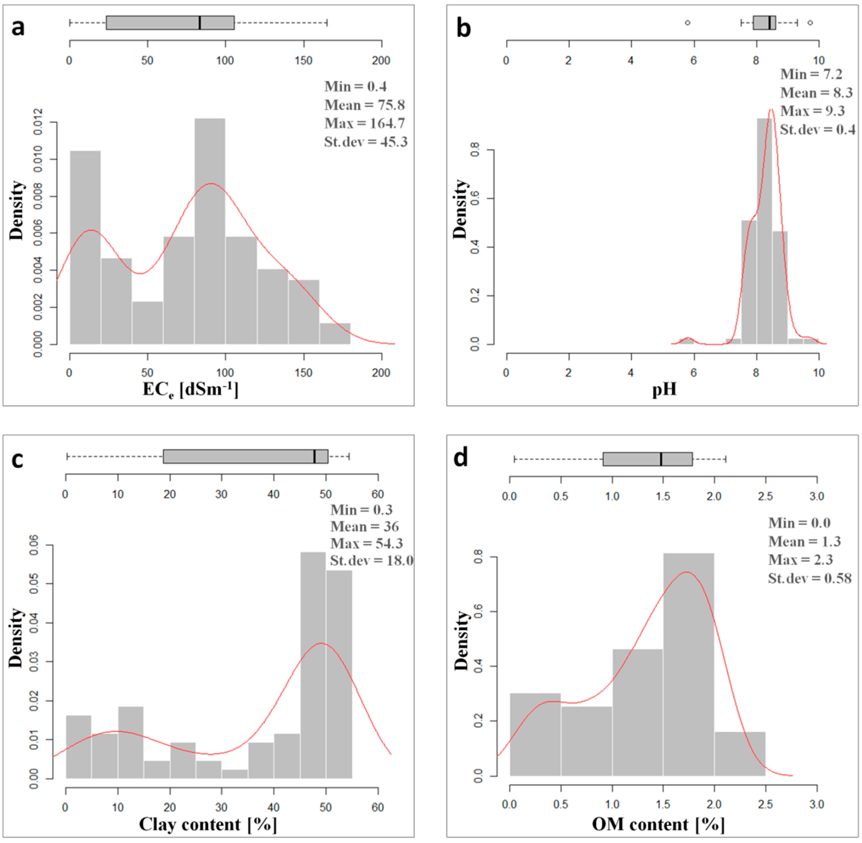
3.1. Soil Properties
3.2. Evaluation of ASTER Data
| pH | ECe | Clay | OM | |
|---|---|---|---|---|
| dSm−1 | % | % | ||
| Min | 7.2 | 0.4 | 0.3 | 0.00 |
| 1st Qu | 8.1 | 36.0 | 19.1 | 0.90 |
| Median | 8.4 | 83.3 | 47.7 | 1.40 |
| Mean | 8.3 | 75.8 | 36.3 | 1.30 |
| 3st Qu | 8.6 | 104.9 | 50.3 | 1.70 |
| Max | 9.3 | 164.7 | 54.3 | 2.30 |
| SD | 0.4 | 45.3 | 18.0 | 0.58 |

3.3. Prediction of Soil Properties
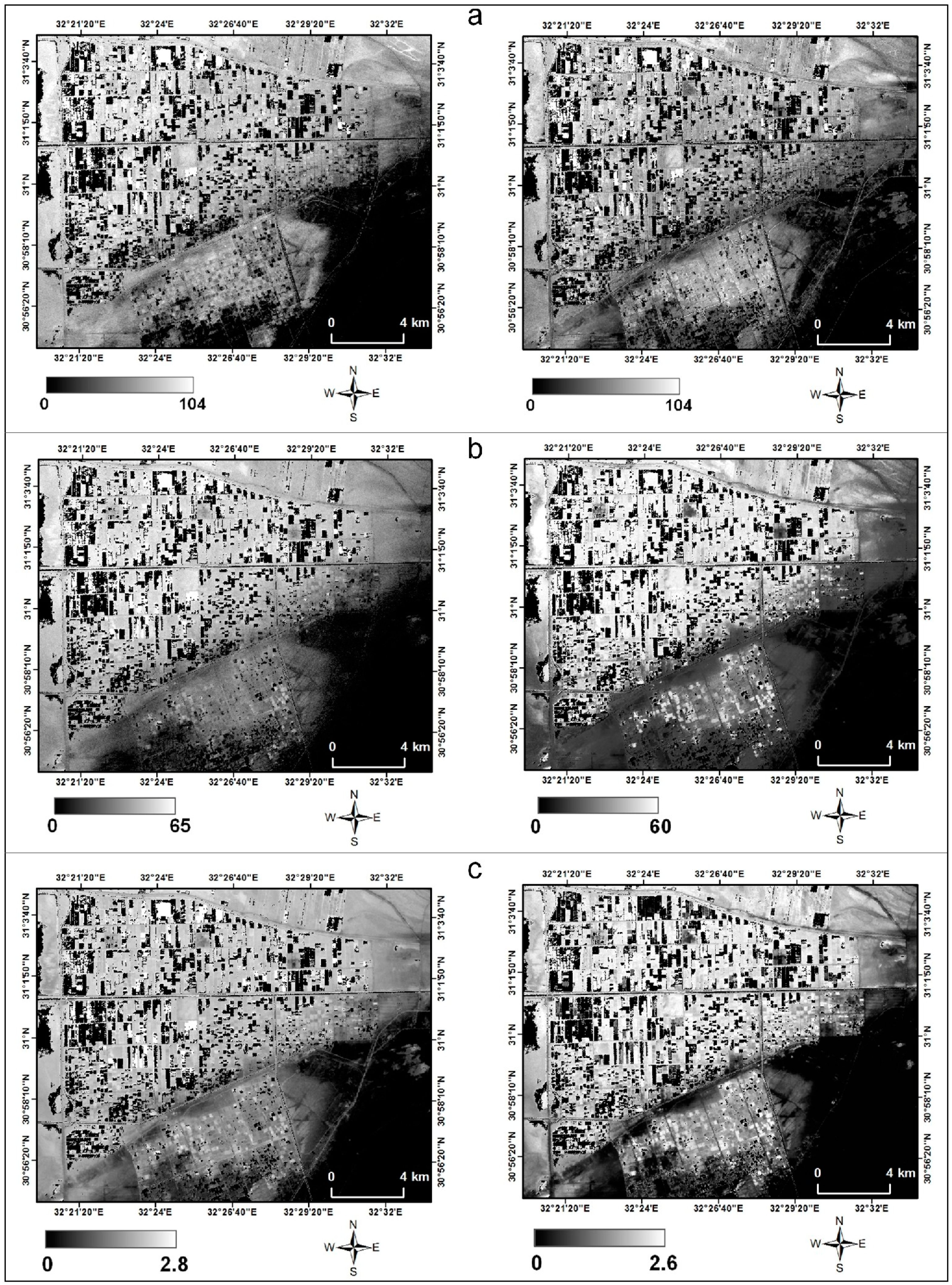
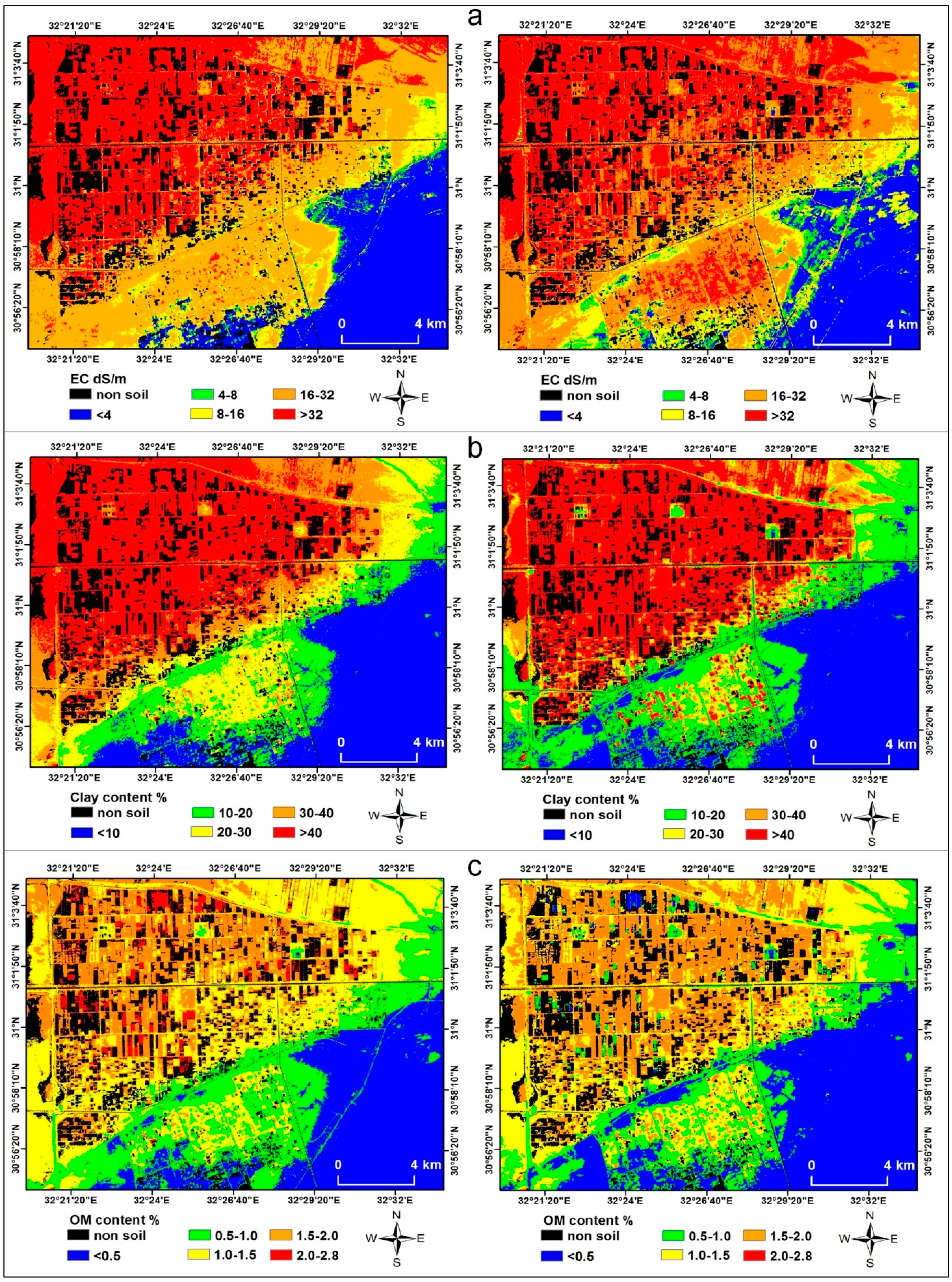
3.4. Mapping of Soil Properties

| PLSR | MARS | |||||||
|---|---|---|---|---|---|---|---|---|
| Nl | R2 | RMSE | RPD | Nb | R2 | RMSE | RPD | |
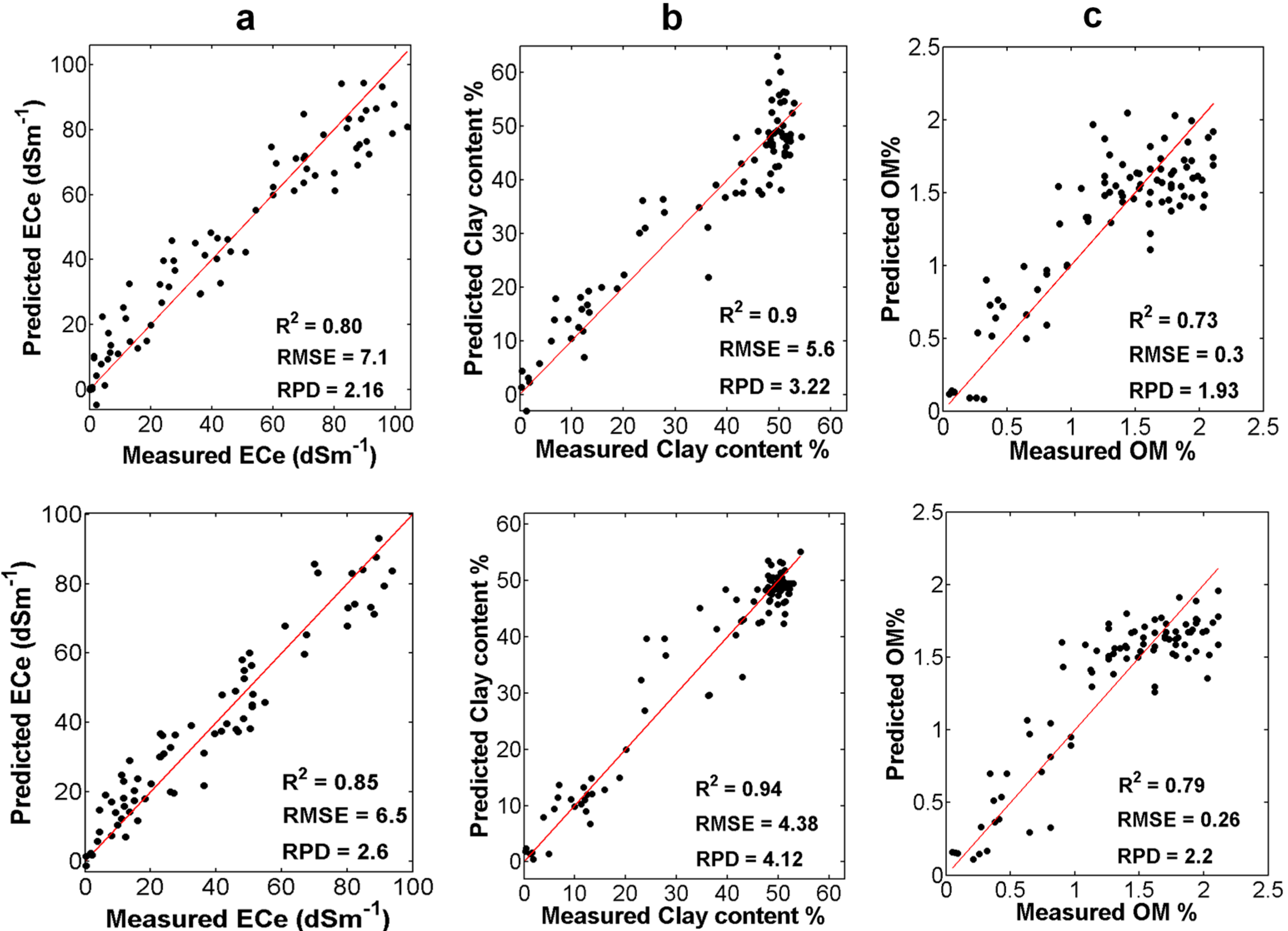
| ECe | 5 | 0.80 | 7.10 | 2.16 | 8 | 0.85 | 6.50 | 2.60 |
| Clay content | 4 | 0.90 | 5.60 | 3.22 | 5 | 0.94 | 4.38 | 4.12 |
| OM | 4 | 0.73 | 0.30 | 1.93 | 8 | 0.79 | 0.26 | 2.20 |


| ECe (dSm−1) | Clay Content (%) | OM (%) | ||||||
|---|---|---|---|---|---|---|---|---|
| PLSR | MARS | PLSR | MARS | PLSR | MARS | |||
| Class | Area (%) | Class | Area (%) | Class | Area (%) | |||
| <4 | 17.54 | 14.87 | <10 | 21.51 | 22.14 | <0.5 | 19.70 | 23.83 |
| 4–8 | 1.51 | 3.24 | 10–20 | 10.90 | 18.74 | 0.5–1 | 15.67 | 13.90 |
| 8–16 | 6.40 | 10.35 | 20–30 | 13.32 | 6.90 | 1–1.5 | 28.30 | 23.95 |
| 16–32 | 30.99 | 27.94 | 30–40 | 12.09 | 7.33 | 1.5–2 | 19.59 | 23.90 |
| >32 | 29.37 | 29.40 | >40 | 27.99 | 30.71 | >2 | 2.55 | 0.20 |

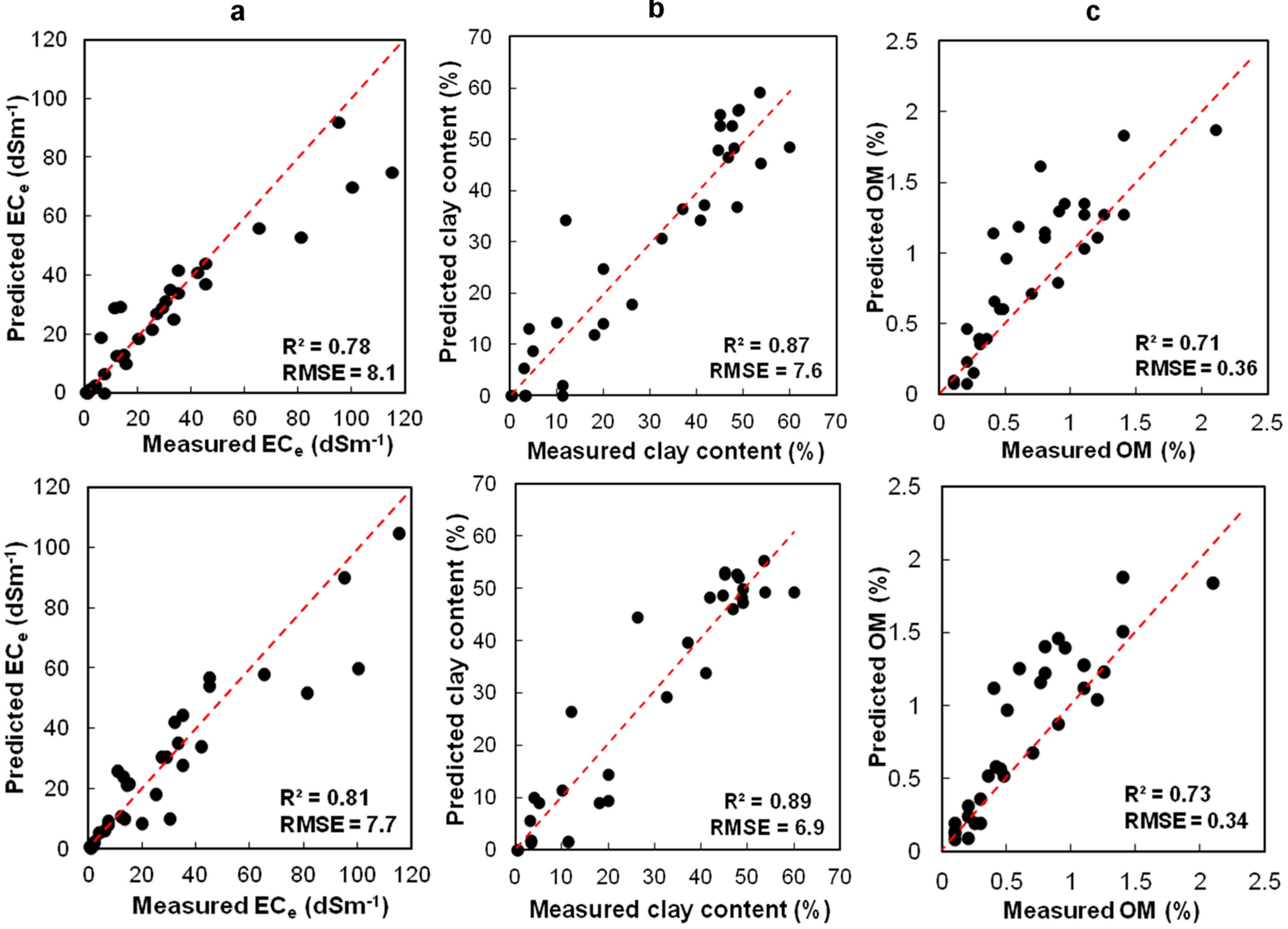
3.5. Validation
4. Discussion
4.1. Evaluation of ASTER Data
4.2. Modeling Soil Properties Using MARS and PLSR Methods
4.3. Soil Mapping and Assessment
5. Conclusions
Acknowledgments
Author Contributions
Conflicts of Interest
References
- Viscarra Rossel, R.A.; Walvoort, D.J.J.; McBratney, A.B.; Janik, L.J.; Skjemstad, J.O. Visible, near infrared, mid infrared or combined diffuse reflectance spectroscopy for simultaneous assessment of various soil properties. Geoderma 2006, 131, 59–75. [Google Scholar]
- Grunwald, S. The current state of digital soil mapping and what is next. In Digital Soil Mapping: Bridging Research, Production and Environmental Applications; Boetinger, J.L., Howell, D.W., Moore, A.C., Hartemink, A.E., Kienst-Brown, S., Eds.; Springer: Heidelberg, Germany, 2010; pp. 3–12. [Google Scholar]
- Vasques, G.M.; Grunwald, S.; Sickman, J.O. Comparison of multivariate methods for inferential modeling of soil carbon using visible/near-infrared spectra. Geoderma 2008, 146, 14–25. [Google Scholar] [CrossRef]
- Mulder, V.L.; de Bruin, S.; Weyermann, J.; Kokaly, R.F.; Schaepman, M.E. Characterizing regional soil mineral composition using spectroscopy and geostatistics. Remote Sens. Environ. 2013, 139, 415–429. [Google Scholar] [CrossRef]
- Obade, V.D.P.; Lal, R. Assessing land cover and soil quality by remote sensing and geographical information systems (GIS). Catena 2013, 104, 77–92. [Google Scholar] [CrossRef]
- Galvdo, L.S.; Vitorello, I.; Formaggio, A.R. Relationships of spectral reflectance and color among surface and subsurface horizons of tropical soil profiles. Remote Sens. Environ. 1997, 61, 24–33. [Google Scholar] [CrossRef]
- Metternicht, G.I.; Zinck, J.A. Remote sensing of soil salinity: Potentials and constraints. Remote Sens. Environ. 2003, 85, 1–20. [Google Scholar] [CrossRef]
- Ge, Y.; Thomasson, J.A.; Sui, R. Remote sensing of soil properties in precision agriculture: A review. Front. Earth Sci. 2011, 5, 229–238. [Google Scholar]
- Mulder, V.L.; de Bruin, S.; Schaepman, M.E.; Mayr, T.R. The use of remote sensing in soil and terrain mapping—A review. Geoderma 2011, 162, 1–19. [Google Scholar] [CrossRef]
- Farifteh, J.; Farshad, A.; George, R.J. Assessing salt-affected soils using remote sensing, solute modelling, and geophysics. Geoderma 2006, 130, 191–206. [Google Scholar] [CrossRef]
- Metternicht, G.I.; Zinck, J.A. Remote Sensing of Soil Salinization: Impact on Land Management; CRC Press: Boca Raton, FL, USA, 2008; p. 337. [Google Scholar]
- Khan, N.M.; Rastoskuev, V.V.; Sato, Y.; Shiozawa, S. Assessment of hydrosaline land degradation by using a simple approach of remote sensing indicators. Agric. Water Manag. 2005, 77, 96–109. [Google Scholar] [CrossRef]
- Fernández-Buces, N.; Siebe, C.; Cram, S.; Palacio, J.L. Mapping soil salinity using a combined spectral response index for bare soil and vegetation: A case study in the former lake Texcoco, Mexico. J. Arid Environ. 2006, 65, 644–667. [Google Scholar] [CrossRef]
- Huang, X.; Senthilkumar, S.; Kravchenko, A.; Thelen, K.; Qi, J. Total carbon mapping in glacial till soils using near-infrared spectroscopy, Landsat imagery and topographical information. Geoderma 2007, 141, 34–42. [Google Scholar] [CrossRef]
- Judkins, G.; Myint, S. Spatial variation of soil salinity in the Mexicali Valley, Mexico: Application of a practical method for agricultural monitoring. Environ. Manag. 2012, 50, 478–89. [Google Scholar] [CrossRef]
- Abrams, M.; Hook, S.; Ramachandran, B. ASTER User Handboek; Jet Propulsion Laboratory: Pasadena, CA, USA, 2002. [Google Scholar]
- Al-khaier, F. Soil Salinity Detection Using Satellite Remote Sensing. Master’s Thesis, Faculty of Geo-Information Science and Earth Observation of the University of Twente, Twente, The Netherlands, 2003. [Google Scholar]
- Melendez-Pastor, I.; Navarro-Pedreño, J.; Koch, M.; Gómez, I. Applying imaging spectroscopy techniques to map saline soils with ASTER images. Geoderma 2010, 158, 55–65. [Google Scholar] [CrossRef]
- Breunig, F.M.; Galvão, L.S.; Formaggio, A.R. Detection of sandy soil surfaces using ASTER-derived reflectance, emissivity and elevation data: Potential for the identification of land degradation. Int. J. Remote Sens. 2008, 29, 1833–1840. [Google Scholar] [CrossRef]
- Luleva, M.I. Identification of Soil Property Variation Using Spectral and Statistical Analyses on Field and ASTER Data. A Case Study of Tunisia Master’s Thesis, Faculty of Geo-Information Science and Earth Observation of the University of Twente, Twente, The Netherlands, 2007. [Google Scholar]
- Sumfleth, K.; Duttmann, R. Prediction of soil property distribution in paddy soil landscapes using terrain data and satellite information as indicators. Ecol. Indic. 2008, 8, 485–501. [Google Scholar] [CrossRef]
- Rivero, R.G.; Grunwald, S.; Binford, M.W.; Osborne, T.Z. Integrating spectral indices into prediction models of soil phosphorus in a subtropical wetland. Remote Sens. Environ. 2009, 113, 2389–2402. [Google Scholar] [CrossRef]
- Piekarczyk, J.; Kaźmierowski, C.; Królewicz, S. Relationships between soil properties of the abandoned fields and spectral data derived from the advanced spaceborne thermal emission and reflection radiometer (ASTER). Adv. Space Res. 2012, 49, 280–291. [Google Scholar] [CrossRef]
- Patkin, K.; Banin, A.; Karnieli, A. Mapping of several soil properties using DAIS-7915 hyperspectral scanner data—A case study over clayey soils in Israel. Int. J. Remote Sens. 2002, 23, 1043–1062. [Google Scholar] [CrossRef]
- Dehaan, R.; Taylor, G.R. Image-derived spectral endmembers as indicators of salinisation. Int. J. Remote Sens. 2003, 24, 775–794. [Google Scholar] [CrossRef]
- Farifteh, J.; van der Meer, F.; Atzberger, C.; Carranza, E.J.M. Quantitative analysis of salt-affected soil reflectance spectra: A comparison of two adaptive methods (PLSR and ANN). Remote Sens. Environ. 2007, 110, 59–78. [Google Scholar] [CrossRef]
- Elnaggar, A.A.; Noller, J.S. Application of remote-sensing data and decision-tree analysis to mapping salt-affected soils over large areas. Remote Sens. 2010, 2, 151–165. [Google Scholar] [CrossRef]
- Moreira, L.; Dos Santos Teixeira, A.; Galvão, L. Laboratory salinization of brazilian alluvial soils and the spectral effects of Gypsum. Remote Sens. 2014, 6, 2647–2663. [Google Scholar] [CrossRef]
- Demattê, J.A.M.; Fiorio, P.R.; Araújo, S.R. Variation of routine soil analysis when compared with hyperspectral narrow band sensing method. Remote Sens. 2010, 2, 1998–2016. [Google Scholar] [CrossRef]
- Gomez, C.; Viscarra Rossel, R.A.; McBratney, A.B. Soil organic carbon prediction by hyperspectral remote sensing and field vis-NIR spectroscopy: An Australian case study. Geoderma 2008, 146, 403–411. [Google Scholar] [CrossRef]
- Stevens, A.; Udelhoven, T.; Denis, A.; Tychon, B.; Lioy, R.; Hoffmann, L.; van Wesemael, B. Measuring soil organic carbon in croplands at regional scale using airborne imaging spectroscopy. Geoderma 2010, 158, 32–45. [Google Scholar] [CrossRef]
- Lu, P.; Wang, L.; Niu, Z.; Li, L.; Zhang, W. Prediction of soil properties using laboratory VIS-NIR spectroscopy and Hyperion imagery. J. Geochem. Explor. 2013, 132, 26–33. [Google Scholar] [CrossRef]
- Peng, X.; Shi, T.; Song, A.; Chen, Y.; Gao, W. Estimating soil organic carbon using VIS/NIR spectroscopy with SVMR and SPA methods. Remote Sens. 2014, 6, 2699–2717. [Google Scholar] [CrossRef]
- Selige, T.; Böhner, J.; Schmidhalter, U. High resolution topsoil mapping using hyperspectral image and field data in multivariate regression modeling procedures. Geoderma 2006, 136, 235–244. [Google Scholar] [CrossRef]
- Viscarra Rossel, R.A.; Cattle, S.R.; Ortega, A.; Fouad, Y. In situ measurements of soil colour, mineral composition and clay content by VIS-NIR spectroscopy. Geoderma 2009, 150, 253–266. [Google Scholar]
- Eisele, A.; Lau, I.; Hewson, R.; Carter, D.; Wheaton, B.; Ong, C.; Cudahy, T.J.; Chabrillat, S.; Kaufmann, H. Applicability of the thermal infrared spectral region for the prediction of soil properties across semi-arid agricultural landscapes. Remote Sens. 2012, 4, 3265–3286. [Google Scholar] [CrossRef]
- Gerighausen, H.; Menz, G.; Kaufmann, H. Spatially explicit estimation of clay and organic carbon content in agricultural soils using multi-annual imaging spectroscopy data. Appl. Environ. Soil Sci. 2012, 2012, 1–23. [Google Scholar]
- Gomez, C.; Lagacherie, P.; Coulouma, G. Regional predictions of eight common soil properties and their spatial structures from hyperspectral VIS-NIR data. Geoderma 2012. [Google Scholar] [CrossRef]
- Ben-Dor, E.; Goldlshleger, N.; Benyamini, Y.; Agassi, M.; Blumberg, D.G. The spectral reflectance properties of soil structural crusts in the 1.2- to 2.5-µm spectral region. Soil Sci. Soc. Am. J. 2003, 67, 289–299. [Google Scholar] [CrossRef]
- Baumgardner, M.F.; Silva, L.F.; Biehl, L.L.; Stoner, E.R. Reflectance properties of soils. Adv. Agron. 1985, 38, 1–44. [Google Scholar]
- Palacios-orueta, A.; Ustin, S.L. Remote sensing of soil properties in the Santa Monica Mountains I. spectral analysis. Remote Sens. Environ. 1998, 65, 170–183. [Google Scholar] [CrossRef]
- Friedl, M.; McIver, D.; Hodges, J.C.; Zhang, X.; Muchoney, D.; Strahler, A.; Woodcock, C.; Gopal, S.; Schneider, A; Cooper, A.; et al. Global land cover mapping from MODIS: Algorithms and early results. Remote Sens. Environ. 2002, 83, 287–302. [Google Scholar] [CrossRef]
- Steffens, M.; Kohlpaintner, M.; Buddenbaum, H. Fine spatial resolution mapping of soil organic matter quality in a Histosol profile. Eur. J. Soil Sci. 2014. [Google Scholar] [CrossRef]
- Keshava, N.; Mustard, J.F. Spectral unmixing. IEEE Signal Process. Mag. 2002, 19, 44–57. [Google Scholar] [CrossRef]
- Hewson, R.D.; Cudahy, T.J.; Jones, M.; Thomas, M. Investigations into soil composition and texture using infrared spectroscopy (2–14 m). Appl. Environ. Soil Sci. 2012, 2012, 1–12. [Google Scholar] [CrossRef]
- Clark, R.N. Imaging spectroscopy: Earth and planetary remote sensing with the USGS Tetracorder and expert systems. J. Geophys. Res. 2003. [Google Scholar] [CrossRef]
- Viscarra Rossel, R.A.; Chen, C. Digitally mapping the information content of visible-near infrared spectra of surficial Australian soils. Remote Sens. Environ. 2011, 115, 1443–1455. [Google Scholar] [CrossRef]
- Wold, S.; Sjostrom, M.; Eriksson, L. PLS-regression: A basic tool of chemometrics. Chemom. Intell. Lab. Syst. 2001, 58, 109–130. [Google Scholar] [CrossRef]
- Weng, Y.; Gong, P.; Zhu, Z. Reflectance spectroscopy for the assessment of soil salt content in soils of the Yellow River Delta of China. Int. J. Remote Sens. 2008, 29, 5511–5531. [Google Scholar] [CrossRef]
- Sidike, A.; Zhao, S.; Wen, Y. Estimating soil salinity in Pingluo County of China using QuickBird data and soil reflectance spectra. Int. J. Appl. Earth Obs. Geoinf. 2014, 26, 156–175. [Google Scholar] [CrossRef]
- Steffens, M.; Buddenbaum, H. Laboratory imaging spectroscopy of a stagnic Luvisol profile—High resolution soil characterisation, classification and mapping of elemental concentrations. Geoderma 2013, 195–196, 122–132. [Google Scholar] [CrossRef]
- Weng, Y.; Gong, P.; Zhu, Z. Soil salt content estimation in the Yellow River delta with satellite hyperspectral data. Can. J. Remote Sens. 2008, 34, 259–270. [Google Scholar]
- Friedman, J.H. Multivariate adaptive regressions splines. Ann. Stat. 1991, 19, 1–67. [Google Scholar] [CrossRef]
- Bilgili, A.V.; van Es, H.M.; Akbas, F.; Durak, A.; Hively, W.D. Visible-near infrared reflectance spectroscopy for assessment of soil properties in a semi-arid area of Turkey. J. Arid Environ. 2010, 74, 229–238. [Google Scholar] [CrossRef]
- Felicísimo, Á.M.; Cuartero, A.; Remondo, J.; Quirós, E. Mapping landslide susceptibility with logistic regression, multiple adaptive regression splines, classification and regression trees, and maximum entropy methods: A comparative study. Landslides 2012, 10, 175–189. [Google Scholar]
- Miska, L.; Jan, H. Evaluation of current statistical approaches for predictive geomorphological mapping. Geomorphology 2005, 67, 299–315. [Google Scholar] [CrossRef]
- Samui, P.; Kurup, P. Multivariate adaptive regression spline (MARS) and least squares support vector machine (LSSVM) for OCR prediction. Soft Comput. 2012, 16, 1347–1351. [Google Scholar] [CrossRef]
- Nawar, S.; Buddenbaum, H.; Hill, J.; Kozak, J. Modeling and mapping of soil salinity with reflectance spectroscopy and Landsat data using two quantitative methods (PLSR and MARS). Remote Sens. 2014, 6, 10813–10834. [Google Scholar] [CrossRef]
- Nawar, S.; Buddenbaum, H.; Hill, J. Estimation of soil salinity using three quantitative methods based on visible and near-infrared reflectance spectroscopy: A case study from Egypt. Arab. J. Geosci. 2014. [Google Scholar] [CrossRef]
- Nawar, S.; Reda, M.; Farag, F.; El-Nahry, A. Mapping soil salinity in El-Tina plain in Egypt using geostatistical approach. In Proceedings of the 2011 Geoinformatics Forum Salzburg, Salzburg, Austria, 5–8 July 2011.
- Aly, E.H.M. Pedological Studies on Some Soils Along El-Salam Canal, North East of Egypt. Ph.D. Thesis, Ain Shams University, Cairo, Egypt, 2005. [Google Scholar]
- El Afandi, G.; Morsy, M.; El Hussieny, F. Heavy rainfall simulation over Sinai Peninsula using the weather research and forecasting Model. Int. J. Atmos. Sci. 2013, 2013, 1–11. [Google Scholar]
- Kilmer, V.J.; Alexander, L.T. Methods of making mechanical analysis of soils. Soil Sci. 1949, 68, 15–24. [Google Scholar] [CrossRef]
- Jackson, M.L. Soil Chemical Analysis; Prentice-Hall of India Private Limited: New Delhi, India, 1973; p. 498. [Google Scholar]
- Nelson, D.W.; Sommers, L.E. Total carbon, organic carbon, and organic matter. In Methods of Soil Analysis Part 2. Chemical and Microbiological Properties, 2nd ed.; Page, A.L., Miller, R.H., Keeney, D.R., Baker, D.E., Ellis, R., Jr., Rhoades, J.D., Eds.; American Society of Agronomy: Madison, WI, USA, 1982; pp. 539–579. [Google Scholar]
- California Institute of Technology, Advanced Spaceborne Thermal Emission and Reflection Radiometer: ASTER Instrument Subsystems. Available online: http://asterweb.jpl.nasa.gov/instrument.asp (accessed on 20 October 2014).
- Badreldin, N.; Frankl, A.; Goossens, R. Assessing the spatio-temporal dynamics of the vegetation cover as an indicator of desertification in Egypt using multi-temporal MODIS satellite images. Arab. J. Geosci. 2014, 7, 4461–4475. [Google Scholar] [CrossRef]
- Frazier, B. Satellite mapping. In Encyclopedia of Soil Science, 2nd ed.; Lal, R., Ed.; Taylor & Francis Group: New York, NY, USA, 2006; Volume 2, pp. 1542–1545. [Google Scholar]
- Ben-Dor, E.; Chabrillat, S.; Demattê, J.A.M.; Taylor, G.R.; Hill, J.; Whiting, M.L.; Sommer, S. Using Imaging Spectroscopy to study soil properties. Remote Sens. Environ. 2009, 113, S38–S55. [Google Scholar] [CrossRef]
- Richter, R.; Schläpfer, D. Atmospheric/Topographic Correction for Satellite Imagery, ATCOR-2/3 User Guide; DLR, Germany’s Aerospace Research Center and Space Agency: Wessling, Germany, 2013; p. 224. [Google Scholar]
- Exelis Visual Information Solutions. ENVI Tutorials. Available online: http://www.exelisvis.com/docs/Tutorials.html (accessed on 26 May 2013).
- Shepherd, K.D.; Walsh, M.G. Development of reflectance spectral libraries for characterization of soil properties. Soil Sci. Soc. Am. J. 2002, 66. [Google Scholar] [CrossRef]
- Yang, C.C.; Prasher, S.O.; Lacroix, R.; Kim, S.H. A Multivariate adaptive regression splines model for simulation of pesticide transport in soils. Biosyst. Eng. 2003, 86, 9–15. [Google Scholar] [CrossRef]
- Bilgili, A.V.; Cullu, M.A.; van Es, H.; Aydemir, A.; Aydemir, S. The use of hyperspectral visible and near infrared reflectance spectroscopy for the characterization of salt-affected soils in the Harran Plain, Turkey. Arid Land Res. Manag. 2011, 25, 19–37. [Google Scholar] [CrossRef]
- Hastie, T.; Tibshirani, R.; Friedman, J. The Elements of Statistical Learning: Data Mining, Inference, and Prediction, 2nd ed.; Springer-Verlag: New York, NY, USA, 2009; p. 763. [Google Scholar]
- Vidoli, F. Evaluating the water sector in Italy through a two stage method using the conditional robust nonparametric frontier and multivariate adaptive regression splines. Eur. J. Oper. Res. 2011, 212, 583–595. [Google Scholar] [CrossRef]
- Jekabsons, G. ARESLab Adaptive Regression Splines Toolbox for Matlab/Octave. 2011, pp. 1–19. Available online: http://www.cs.rtu.lv/jekabsons/regression.html (accessed on 30 January 2013).
- Geladi, P.; Kowalski, B.R. Partial least-squares regression: A tutorial. Anal. Chim. Acta 1986, 185, 1–17. [Google Scholar] [CrossRef]
- Chang, C.; Laird, D.; Mausbach, M.J. Near-infrared reflectance spectroscopy—Principal components regression analyses of soil properties analyses of soil properties. Soil Sci. Soc. Am. J. 2001, 65, 480–490. [Google Scholar] [CrossRef]
- Karunaratne, S.B.; Bishop, T.F.A.; Baldock, J.A.; Odeh, I.O.A. Catchment scale mapping of measureable soil organic carbon fractions. Geoderma 2014, 219–220, 14–23. [Google Scholar] [CrossRef]
- Mahmoud, E.; Abd EL-Kader, N.; Robin, P.; Akkal-Corfini, N.; Abd El-Rahman, L. Effects of different organic and inorganic fertilizers on cucumber yield and some soil properties. World J. Agric. Sci. 2009, 5, 408–414. [Google Scholar]
- Tangestani, M.H.; Mazhari, N.; Agar, B.; Moore, F. Evaluating Advanced Spaceborne Thermal Emission and Reflection Radiometer (ASTER) data for alteration zone enhancement in a semi-arid area, northern Shahr-e-Babak, SE Iran. Int. J. Remote Sens. 2008, 29, 2833–2850. [Google Scholar] [CrossRef]
- Pour, A.B.; Hashim, M. The application of ASTER remote sensing data to porphyry copper and epithermal gold deposits. Ore Geol. Rev. 2012, 44, 1–9. [Google Scholar] [CrossRef] [Green Version]
- Buhe, A.; Tsuchiya, K.; Kaneko, M.; Ohtaishi, N.; Halik, M. Land cover of oases and forest in XinJiang, China retrieved from ASTER data. Adv. Space Res. 2007, 39, 39–45. [Google Scholar] [CrossRef]
- Buho, H.; Kaneko, M.; Ogawa, K. Correction of NDVI calculated from ASTER L1B and ASTER (AST07) data based on ground measurement. In Advances in Geoscience and Remote Sensing; Jedlovec, G., Ed.; InTech.: Rijeka, Croatia, 2009. [Google Scholar]
- Mashimbye, Z.E.; Cho, M.A.; Nell, J.P.; de Clercq, W.P.; Van Niekerk, A.; Turner, D.P. Model-based integrated methods for quantitative estimation of soil salinity from hyperspectral remote sensing data: A case study of selected South African soils. Pedosphere 2012, 22, 640–649. [Google Scholar] [CrossRef]
- Lagacherie, P.; Baret, F.; Feret, J.B.; Madeira Netto, J.; Robbez-Masson, J.M. Estimation of soil clay and calcium carbonate using laboratory, field and airborne hyperspectral measurements. Remote Sens. Environ. 2008, 112, 825–835. [Google Scholar] [CrossRef]
- Viscarra Rossel, R.A.; McBratney, A.B. Laboratory evaluation of a proximal sensing technique for simultaneous measurement of soil clay and water content. Geoderma 1998, 85, 19–39. [Google Scholar] [CrossRef]
- Barnes, E.M.; Sudduth, K.A.; Hummel, J.W.; Lesch, S.M.; Corwin, D.L.; Yang, C.; Daughtry, C.S.T.; Bausch, W.C. Remote- and ground-based sensor techniques to map soil properties. Photogramm. Eng. Remote Sens. 2003, 69, 619–630. [Google Scholar] [CrossRef]
- Ghasemi, J.B.; Zolfonoun, E. Application of principal component analysis-multivariate adaptive regression splines for the simultaneous spectrofluorimetric determination of dialkyltins in micellar media. Spectrochim. Acta. A. Mol. Biomol. Spectrosc. 2013, 115, 357–363. [Google Scholar] [CrossRef] [PubMed]
- Khoshayand, M.R.; Abdollahi, H.; Shariatpanahi, M.; Saadatfard, A.; Mohammadi, A. Simultaneous spectrophotometric determination of paracetamol, ibuprofen and caffeine in pharmaceuticals by chemometric methods. Spectrochim. Acta. Part A Mol. Biomol. Spectrosc. 2008, 70, 491–499. [Google Scholar] [CrossRef]
- Shamsi, F.S.R.; Zare, S.; Abtahi, S.A. Soil salinity characteristics using moderate resolution imaging spectroradiometer (MODIS) images and statistical analysis. Arch. Agron. Soil Sci. 2013, 59, 471–489. [Google Scholar] [CrossRef]
- Allbed, A.; Kumar, L.; Sinha, P. Mapping and modelling spatial variation in soil salinity in the al hassa oasis based on remote sensing indicators and regression techniques. Remote Sens. 2014, 6, 1137–1157. [Google Scholar] [CrossRef]
- Dobos, E. Albedo. In Encyclopedia of Soil Science; Taylor & Francis: London, UK, 2006; p. 64. [Google Scholar]
- Farag, F.M. Mineral-Chemical Characteristics of the Canal Area. Master’s Thesis, Suez Canal University, Ismailia, Egypt, 1981. [Google Scholar]
- Reda, M. Soil resources and their potentiality in Sinai. In Proceedings of the 1998 Regional Symposium on Agro-technologies Based on Biological Nitrogen Fixation for Desert Agriculture, El-Arish, North Sinai, Egypt, 14–16 April 1998.
- El Hajj, M.; Bégué, A.; Lafrance, B.; Hagolle, O.; Dedieu, G.; Rumeau, M. Relative radiometric normalization and atmospheric correction of a SPOT 5 time series. Sensors 2008, 8, 2774–2791. [Google Scholar] [CrossRef]
- Brus, D.J.; Kempen, B.; Heuvelink, G.B.M. Sampling for validation of digital soil maps. Eur. J. Soil Sci. 2011, 62, 394–407. [Google Scholar] [CrossRef]
- Brodský, L.; Vašát, R.; Klement, A.; Zádorová, T.; Jakšík, O. Uncertainty propagation in VNIR reflectance spectroscopy soil organic carbon mapping. Geoderma 2013, 199, 54–63. [Google Scholar] [CrossRef]
- Nelson, M.A.; Bishop, T.F.A.; Triantafilis, J.; Odeh, I.O.A. An error budget for different sources of error in digital soil mapping. Eur. J. Soil Sci. 2011, 62, 417–430. [Google Scholar] [CrossRef]
© 2015 by the authors; licensee MDPI, Basel, Switzerland. This article is an open access article distributed under the terms and conditions of the Creative Commons Attribution license (http://creativecommons.org/licenses/by/4.0/).
Share and Cite
Nawar, S.; Buddenbaum, H.; Hill, J. Digital Mapping of Soil Properties Using Multivariate Statistical Analysis and ASTER Data in an Arid Region. Remote Sens. 2015, 7, 1181-1205. https://doi.org/10.3390/rs70201181
Nawar S, Buddenbaum H, Hill J. Digital Mapping of Soil Properties Using Multivariate Statistical Analysis and ASTER Data in an Arid Region. Remote Sensing. 2015; 7(2):1181-1205. https://doi.org/10.3390/rs70201181
Chicago/Turabian StyleNawar, Said, Henning Buddenbaum, and Joachim Hill. 2015. "Digital Mapping of Soil Properties Using Multivariate Statistical Analysis and ASTER Data in an Arid Region" Remote Sensing 7, no. 2: 1181-1205. https://doi.org/10.3390/rs70201181