Surface Temperatures at the Continental Scale: Tracking Changes with Remote Sensing at Unprecedented Detail


Abstract
: Temperature is a main driver for most ecological processes, and temperature time series provide key environmental indicators for various applications and research fields. High spatial and temporal resolutions are crucial for detailed analyses in various fields of research. A disadvantage of temperature data obtained by satellites is the occurrence of gaps that must be reconstructed. Here, we present a new method to reconstruct high-resolution land surface temperature (LST) time series at the continental scale gaining 250-m spatial resolution and four daily values per pixel. Our method constitutes a unique new combination of weighted temporal averaging with statistical modeling and spatial interpolation. This newly developed reconstruction method has been applied to greater Europe, resulting in complete daily coverage for eleven years. To our knowledge, this new reconstructed LST time series exceeds the level of detail of comparable reconstructed LST datasets by several orders of magnitude. Studies on emerging diseases, parasite risk assessment and temperature anomalies can now be performed on the continental scale, maintaining high spatial and temporal detail. We illustrate a series of applications in this paper. Our dataset is available online for download as time aggregated derivatives for direct usage in GIS-based applications.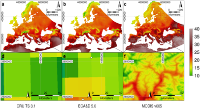
1. Introduction
High spatial and temporal resolution datasets of environmental indicators are crucial requirements for detailed analyses in various fields of research [1–6]. Important environmental indicators are derived from temperature time series [7], since temperature is a main driver for most ecological and environmental processes [8]. Temperature data can be acquired with satellites carrying thermal infrared sensors, which provide continuous coverage of large areas. However, a major disadvantage of available satellite-based temperature data is the occurrence of gaps, especially due to clouds, that must be filled.
1.1. Gridded Temperature Surfaces
Seamless gridded surfaces allow for spatially explicit and detailed analyses, whereas sparse points, such as station readings, are only valid for a single location and its immediate surroundings, leaving, at times, large gaps between stations. Gridded surfaces of environmental indicators are often created by interpolating meteorological point data recorded at ground stations. An alternative to ground station data are data acquired through remote sensing. Examples are the commonly used land surface temperature and emissivity products (LST/E; [9]) from the Moderate Resolution Imaging Sensor (MODIS) instruments onboard the Terra and Aqua satellites, which contain spatialized surfaces with global coverage accompanied by a quality assessment layer. MODIS-Terra data are available from March 2000, onwards, MODIS-Aqua data from July 2002, onwards, with twice-daily temporal resolution for both instruments, MODIS-Terra and MODIS-Aqua. MODIS data have been extensively used in continental-scale studies in a number of different research fields, like wildlife habitat distribution (NDVI [10]), habitat change monitoring (fraction of photosynthetically active radiation [11]) and land cover mapping (various MODIS products [12]). MODIS LST products are available with different spatial and temporal resolutions and always include daytime and nighttime land surface temperature layers. MODIS data are usually made publicly available for download on a NASA server ( https://lpdaac.usgs.gov/data_access) a few days after image acquisition [9].
1.2. Reconstruction of Remotely Sensed Temperature Maps
Surface interpolation approaches using only temperature and no auxiliary data fail to produce realistic results in areas with complex topography [13] when the data points used for interpolation are unevenly distributed, leaving large gaps. Therefore, spatial interpolation methods should not only use the existing LST values, but also auxiliary data as predictors for LST in a statistical model. Predicting LST with auxiliary data can also enhance the spatial detail to the level of the auxiliary data. Temporal interpolation can complement the spatial interpolation of missing values, alleviating the problem of large spatial gaps.
1.3. Previous Approaches
Temperature reconstruction in the temporal domain has previously been performed using Fourier transform by Scharlemann et al. [14], who processed MODIS LST at a full global extent for the years 2001 to 2005 and extracted parameters for the annual, bi-annual and tri-annual cycle with a resolution of 1000 m, thereby reducing 450 grids to 34 parameters. In a different context, temporal interpolation has been performed for NDVI reconstruction using non-linear least squares fits of asymmetric Gaussian model functions [15]. Another temporal interpolation method estimates missing Aqua LST values from Terra LST values and the seasonal average between Aqua LST and Terra LST [16,17]. This method replaces some, but not all, missing values, and the resulting dataset may still not be gap-free. Furthermore, this method has been applied at a national scale, but not a continental scale. Another possibility for temporal reconstruction is presented by a harmonic analysis of time series (HANTS; [18]), which can reconstruct missing values and detect outliers in time series data. Even though HANTS was originally developed for NDVI reconstruction, it can, in theory, also be applied to LST or any other time series showing periodicity. Regarding spatial interpolation, previously applied methods to filter and reconstruct MODIS LST values include 2D [19] and 3D [13] spline interpolation. While being a full reconstruction of all layers, the approach of Neteler et al. [13] was only developed for a small region with very complex topography. It cannot be extended to larger regions, because factors other than topography will become increasingly important when extending the analyzed area towards the continental scale.
For large-extent reconstructed LST time series, the largest study area in terms of the number of grid cells that we are aware of, has been analyzed by Crosson et al. [17], who created a daily merged MODIS Aqua-Terra land surface temperature dataset for the conterminous United States (eight million km2) with 1000-m resolution and 16 million grid cells (the study presented here consists of 415 million grid cells).
Hengl et al. [19] applied a statistical interpolation model, where MODIS LST values were used together with other auxiliary data to predict daily air temperatures. Lin et al. [20] estimated air temperature from MODIS LST and elevation with a multiple regression. The common objective of these two studies is the enhancement of spatial detail with the help of one or more predicting variables in a statistical model. In general, any surface interpolation method, e.g., inverse distance weighting, spline interpolation, kriging, etc., can be applied, but should be combined with a regression approach in order to obtain more realistic results. Our approach includes climate conditions as statistical predictors for LST. For a summary of previous approaches to reconstruct LST time series, see Table 1 [13,14,17,19,21].
Here we present a new method for reconstructing spatio-temporal gaps in remotely sensed land surface temperature (LST) time series at continental scale. Our approach delivers a final product with 250 m spatial resolution and four daily values per pixel position. We have developed an innovative reconstruction method which we applied to larger Europe (see Figure 1a) for all daily MODIS LST data available from 2000 to 2013. To our knowledge, no other method is available for seamless and gap-free daily LST reconstruction at continental scale. For risk modelling, seamless and gap-free datasets of environmental indicators [13], e.g., in order to derive growing degree days [22] or spring warming, are required. Our reconstruction method will enable researchers to use a uniform, gap-free and seamless LST dataset and its derivatives (see Table 2) yielding comparable results that are crucially needed and lacking so far, e.g., for studies on emerging diseases, parasite risk assessment, and temperature anomalies. Furthermore, the presented reconstruction method can easily be adapted to continents different from Europe. The new method presented here differs substantially from previous studies (see below for a comparison) and provides with the creation of a seamless dataset at continental scale an advance over previously published LST datasets.
Our efforts to reconstruct temperature time series for a large area with high detail has been motivated by our involvement in continental-scale projects, in particular the EU/FP7 projects, EDENext ( http://www.edenext.eu/) and EuroWestNile ( http://www.eurowestnile.org/). Both address vector-borne infections in Europe. Furthermore, this new dataset and its derivatives can be used for the assessment of how temperature-influenced agricultural pests spread (e.g., Drosophila suzukii; [23]), the monitoring of heat and cold waves and the identification of temperature anomalies.
2. Materials and Methods
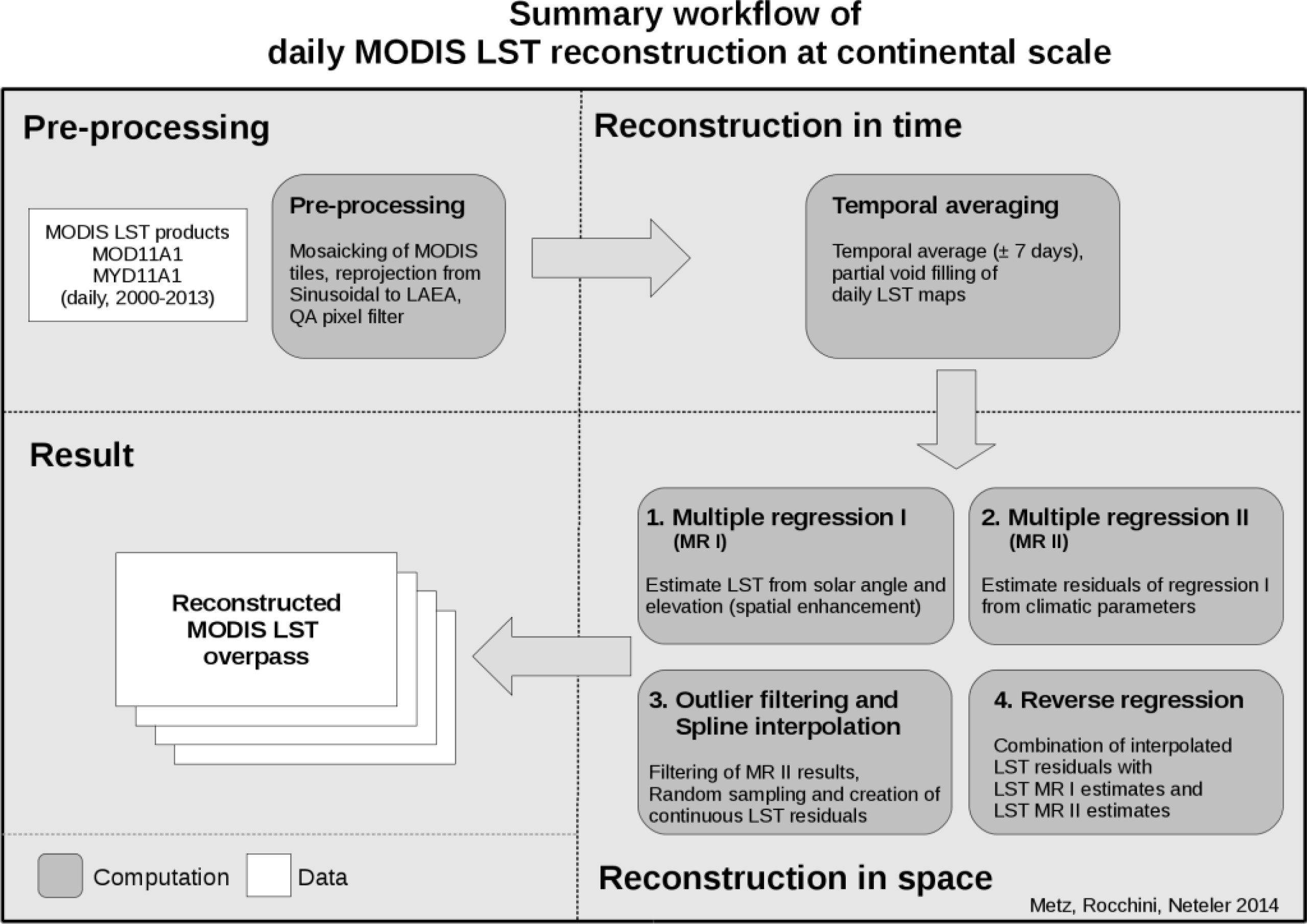
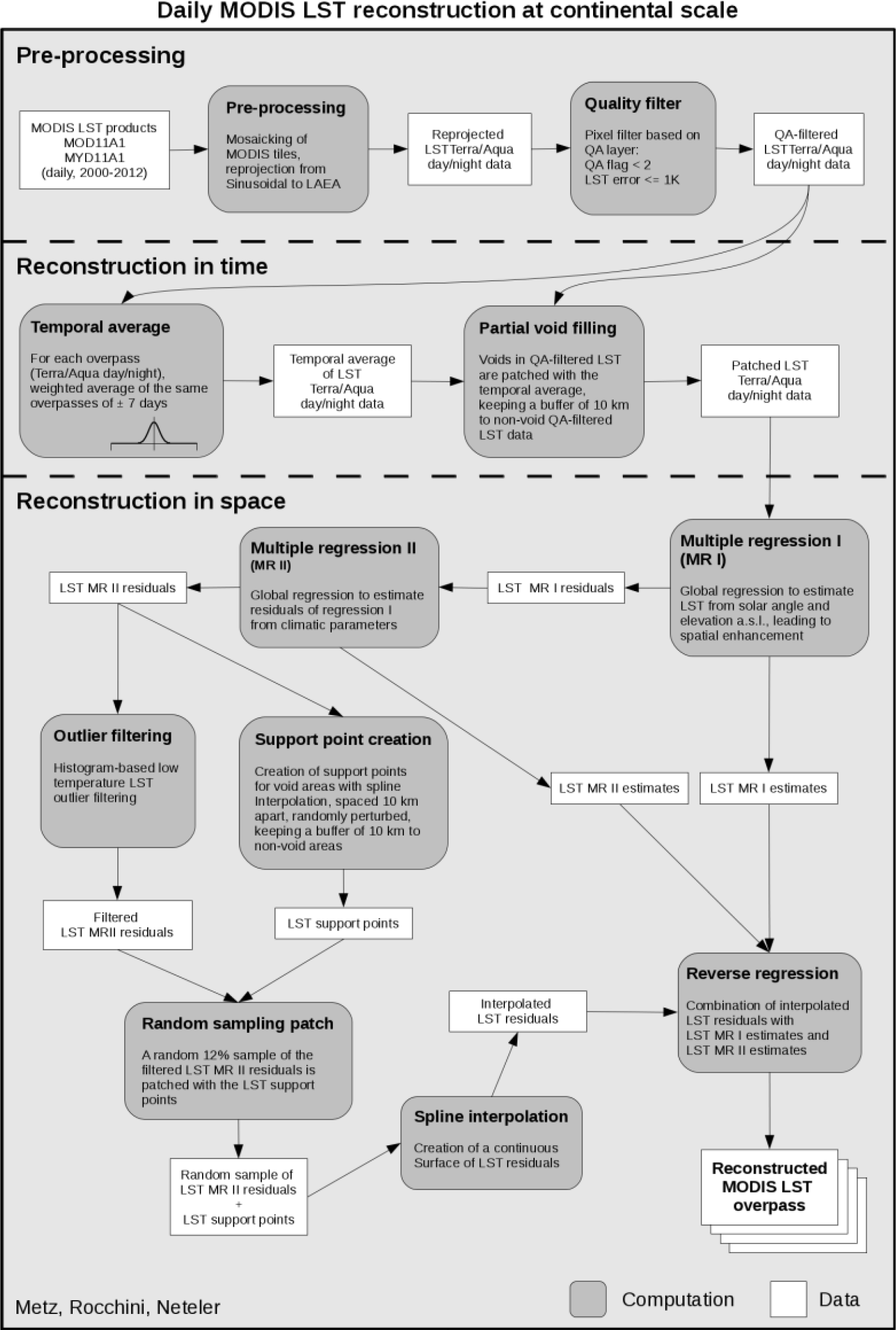
Our study area covers about 12.5 million km2 of land and includes a wide variety of climate zones, ranging from hot, arid zones, to permafrost and from coastal plains to mountains with continental climates. Elevation ranges from 420 m below sea level to 5600 m above sea level. The boundaries are: North: 72°11′19N, South: 23°17′10N, West: 39°53′33W, East: 75°32′30E. At 250-m spatial resolution, this region consists of 415 million grid cells in total, of which 200 million grid cells fall on land and inland water bodies. We used the daily gridded MODIS products with 1000-m spatial resolution (Terra: MOD11A1; and Aqua: MYD11A1; version 005) provided in an equal-area sinusoidal projection. The reconstruction process consists of three steps (see Figure 2 for a summary). In the pre-processing step, raw data are mosaicked, reprojected and filtered with the accompanying quality assessment. In the next step, some, but not all, gaps are removed with temporal averaging. The final and most important step applies spatial statistical interpolation to close the remaining gaps and to enhance the spatial detail.
2.1. Pre-Processing
The raw data (see supplementary Figure S1 for MODIS tile coverage of the study area) were mosaicked and reprojected to Lambert azimuthal equal area (EU LAEA, EPSG code 3035) with 250-m resolution using the MODIS Reprojection Tool (MRT 4.1; https://lpdaac.usgs.gov/tools/modis_reprojection_tool, the gdalwarp command from the Geospatial Data Abstraction Library (GDAL) library might be preferred) with nearest neighbor as the resampling method (supplementary Figure S2: MODIS tile deformation after reprojection). Nearest neighbor sampling was chosen in order to preserve the bit pattern in the quality assessment (QA) band, which would be destroyed by methods, such as linear or cubic interpolation. The spatial oversampling from 1000 m to 250 m reduced artefacts and pixel shifts (supplementary Figure S2). Oversampling and interpolation of sparse points is a well-established method for ground station data (European Climate Assessment and Dataset (ECA&D) [24]; Climatic Research Unit time series (CRU TS) dataset [25]). The reprojected MODIS LST values were then filtered with the LST QA band, such that all grid cells with an LST error larger than 1 K were discarded.
Our LST reconstruction method that we employed here uses a combination of a Gaussian kernel filter in the time domain followed by global regression analysis and spline-based interpolation in the space domain (see the detailed workflow in Figure 3).
2.2. Further Input Data
Oceans were excluded from both the raw and the reconstructed LST maps using the quality assessment of the MODIS NDVI product, MOD13Q1. The quality assessment of the MODIS NDVI product, MOD13Q1, distinguishes between the type of water body, e.g., deep ocean, shallow ocean, deep inland water and shallow inland water, whereas the land water mask derived from MODIS and Shuttle Radar Topography Mission (SRTM) L3 (MOD44W) distinguishes between data sources (SRTM Water Body Dataset, MODIS 250 m water-hits, MODIS 250 m decision-tree, digitized water, mosaic of Antarctica water) instead of types of water bodies. As we needed to distinguish between ocean and inland water bodies, we used the quality assessment information of the MODIS NDVI product, MOD13Q1. The land mask was extended by a buffer of 10 km, because some land areas were erroneously marked as ocean.
We used six additional variables as potential predictors for LST in the regression analysis: elevation, solar angle at noon local time, annual precipitation, mean annual temperature, minimum annual temperature and the range of annual temperature. Elevation was obtained from SRTM v2.1 ( http://dds.cr.usgs.gov/srtm/version2_1/SRTM3/), complemented with gridded global relief data (ETOPO2; http://www.ngdc.noaa.gov/mgg/global/relief/ETOPO2/), for latitudes north of 60° North. Voids in the DEM were filled with spline interpolation. The DEM was interpolated with spatial averaging to match the target resolution of the reconstructed LST data. The solar angle was calculated using the Solar Position and Intensity algorithm of the National Renewable Energy Laboratory (NREL SOLPOS 2.0; [26]). The long-term climatic parameters were calculated from daily gridded datasets of the European Climate Assessment and Dataset (ECA&D [24]). In order to obtain climatically representative indicators, we aggregated daily ECA&D data per year for 30 years from 1980 to 2010 to long-term annual averages for annual precipitation, mean and minimum annual temperature and the range of annual temperature. These parameters describe geographical differences in climate, but should not describe short-term temporal variation, because this information is provided by the MODIS LST data and is to be reconstructed. We used bilinear interpolation to adjust the spatial resolution of the climatic parameters to the resolution of the reconstructed LST data. The four climatic parameters were reduced by means of a principal components analysis. The first two extracted principal components explained more than 95% of the variance of the original system (four climatic variables, see supplementary Table S1) and were used in the reconstruction method instead of the original climatic variables.
2.3. Temporal Pre-Processing
Some of the original LST grids have a very large proportion of missing values (up to 100%). On average, 23% of the non-ocean pixels were valid; see Table 3 for a summary of valid pixels per month. The purpose of the temporal pre-processing is to reduce the size of the spatial gaps in order to make spatial interpolation more accurate. Each map is patched with temporally surrounding original maps considering the same time of day of the preceding and following seven days. If there were no valid values in any of the preceding and following 7 days, the pixel was not temporally reconstructed. The influence of the temporally surrounding maps is weighed with a symmetric Gaussian kernel, such that maps closer in time had a larger weight. In order to keep the influence of the patching low, a grid cell with a missing value is patched only if the nearest valid grid cell was more than 10 km away, and valid values are not altered at all. If an LST grid does not contain any valid values, it is in our method reconstructed by using the temporally nearest reconstructed maps of the same time of day, e.g., only Aqua daytime values were used to estimate a missing Aqua daytime value. The grid was then reconstructed by using the inverse distance weighted average of the closest preceding and the closest following reconstructed grid. Inverse distance weighing was needed, because the temporal distances in days to the preceding grid and the following grid could be different. This step was performed after reconstructing all grids with valid values.
2.4. Spatial Interpolation
After the temporal processing, we combined statistical modeling with spatial interpolation to fill any remaining gaps. A grid-wise multiple regression is performed with elevation and solar angle as predictors for LST values, providing estimates and residuals of the LST values. If the temperature lapse rate (the rate of temperature decrease with increasing elevation) exceeded physical and meteorological constraints, we decided to reconstruct the LST dataset by using the temporally nearest reconstructed maps of the same time of day. Rolland [27] studied (unrelated to spatial LST interpolation) lapse rates of minimum, mean and maximum air temperatures in the Trentino-South Tyrol region, finding lapse rates from −0.40 °C/100 m to −0.75 °C/100 m (monthly values). If the lapse rate was found to be outside this range, the LST grid was not reconstructed and instead estimated from LST grids of the previous and next days; otherwise, the residuals of the first regression were predicted with the two principal components describing climate in a second regression, providing a second set of estimates and residuals. Outliers in MODIS V005 LST data typically only appear in the negative degree Celsius range, as being caused by undetected clouds [13]. A global filter for the whole study area on the original LST values is not adequate, because of the large range of valid LST values. One possibility would be to remove outliers in the LST values with a moving window filter, but this is problematic, because spatial gaps with missing values were sometimes very large (thousands of km2). Another possibility is to apply a global filter to the residuals of the second regression, where variation due to geographic location and climatic conditions has been removed. The lower threshold for valid residual values was calculated from quartiles according to Equation (1) (after [13]):
A random selection of 12% (approximately two pixels for each original 1 km × 1 km pixel; after [13]) of the filtered residuals (error terms) of the second regression was then interpolated using a B-spline approach (in GRASS GIS 7: r.resamp.bspline; based on v.surf.bspline of [28], optimized for large raster data) to obtain a seamless, smooth surface from sparse raster points. This step also performed the actual spatial enhancement. Finally, the filtered and interpolated residuals were converted back to real LST values by adding the estimates and offsets of the two regressions to the residuals. This approach of combining a statistical regression model with spatial interpolation is comparable to regression kriging (as suggested by [29]).
2.5. Validation
For validation of the spatial enhancement, we compared original and reconstructed MODIS LST values for twelve days in the years 2003 and 2010. The twelve sampling days were evenly spread over the respective year in order to cover all seasons.
For validation of the gap-filling procedure, we inserted artificial gaps into original LST data, reconstructed these “degraded” LST data and compared the reconstructed LST values with the original values without artificial gaps. This procedure was applied to the same twelve days, both in the year 2003 and in the year 2010, as in the first evaluation. The inserted gaps were taken from a day with a large amount of missing values in order to simulate realistic gaps. A random selection of pixels would have resulted in artificial gaps of 1 pixel size, which is not realistic.
2.6. Computing Environment
Data processing was performed on a high performance computing (HPC) system with 300 nodes with Scientific Linux 6.4 ( http://www.scientificlinux.org) as the operating system. Reconstructing time series with a manual or even interactive method is often not feasible, because the amount of time series data can be huge (as of December 2013, more than 17,000 MODIS LST maps are available for each tile). Therefore, we automated the complete workflow to process the dataset parallelized on our HPC system. All calculations were done in GRASS GIS version 7 [30], with the exception of the initial MODIS LST mosaicking and reprojection, which was done with the MODIS Reprojection Tool (MRT 4.1, https://lpdaac.usgs.gov/tools/modis_reprojection_tool) using pyMODIS as the download library ( http://pymodis.fem-environment.eu/). Since common statistical software is not able to process the six input grids (LST, altitude, solar angle, two principal components, ocean mask) with about 400 million grid cells each, we used a pure GIS environment optimized for handling large spatial datasets in the billions of pixel range. Here, the free and open source software license [30,31] of GRASS GIS was essential for the implementation of enhancements relevant to large dataset processing (large file support (LFS), external memory, code optimization, statistical analysis of spatial data, optimization for HPC systems). We developed a new module to perform multiple regressions on raster data using innovative GIS data handling concepts (now included in GRASS GIS 7: r.regression.multi module), which minimizes hardware resource requirements, in particular memory consumption, and maximizes processing speed. The results were tested against and found to be identical to the results obtained with R statistical package 2.14 [32] when tested with smaller, but representative, datasets (the size was limited due to R’s memory management constraints). Other routines required for the Europe-wide LST reconstruction were optimized for large datasets where needed, e.g., the principal component analysis within GRASS GIS (i.pca module), suitable for datasets in the billions of pixel range. We integrated all enhancements in GRASS GIS 7, which can be freely downloaded from the project website ( http://grass.osgeo.org/download/software/).
3. Results
3.1. The Reconstructed Daily MODIS LST Dataset
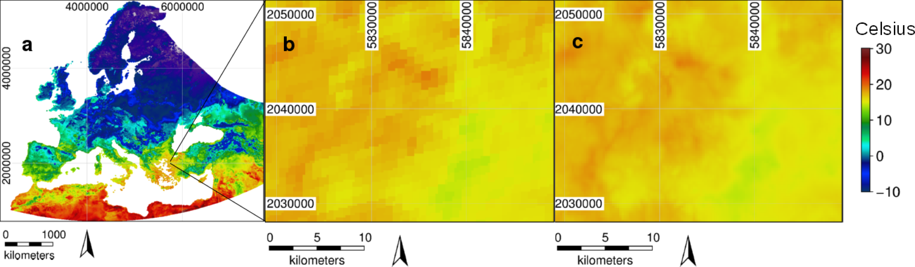
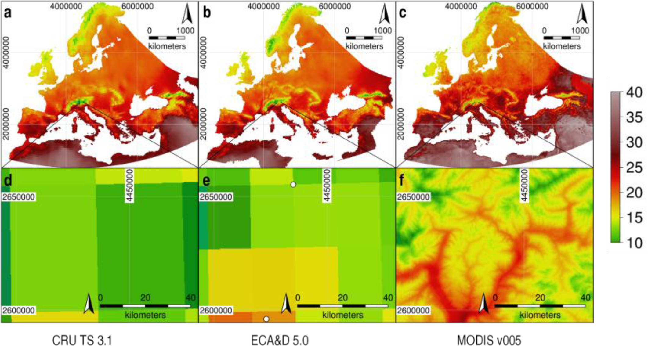
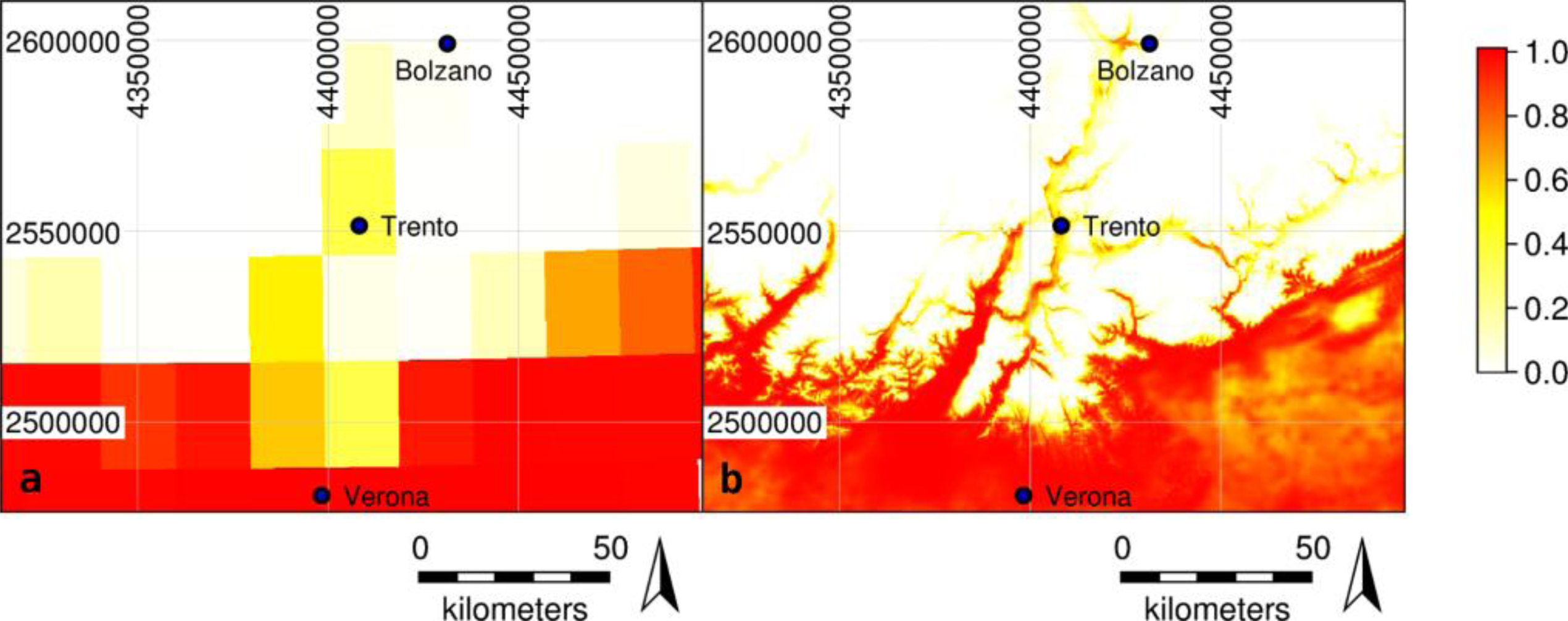
The reconstructed daily MODIS LST time series provides substantially more spatial detail than other existing temperature time series datasets. Figure 4 shows the European heat wave in July 2003, from temperature surfaces interpolated from station data (CRU TS and ECA&D), as well as from our enhanced MODIS LST dataset. Comparing original and reconstructed data, the original data show distinct blocks (Figure 1b) corresponding to the original 1000-m grid cells, whereas the reconstructed LST data are both smoother and more closely follow the terrain features. Slopes in particular are more realistically represented in the reconstructed data. The enhancement of the spatial detail is primarily caused by elevation as a predictor of LST in the regression model. Spatial enhancement of the reconstructed LST grids (Figure 1c) was primarily caused by elevation; because of the predictors used only for elevation, the local variation can be higher than the continental variation; the difference in, e.g., the solar angle increases with the north-south distance, whereas the difference in elevation of two nearby locations may or may not be larger than the difference in elevation of two locations farther apart from each other. Since we are working on the continental scale, other factors considering the continental scale need to be taken into account in order to achieve small-scale spatial enhancement using elevation. For example, using only elevation as a predictor would not work on the continental scale, because the temperature at a given height is different between the Pyrenees and the North Scandinavian mountains and can, thus, not be predicted by elevation alone.
We have made the dataset available for download in the form of temperature-based bioclimatic variables and monthly averages (see Table 2).
3.2. Validation
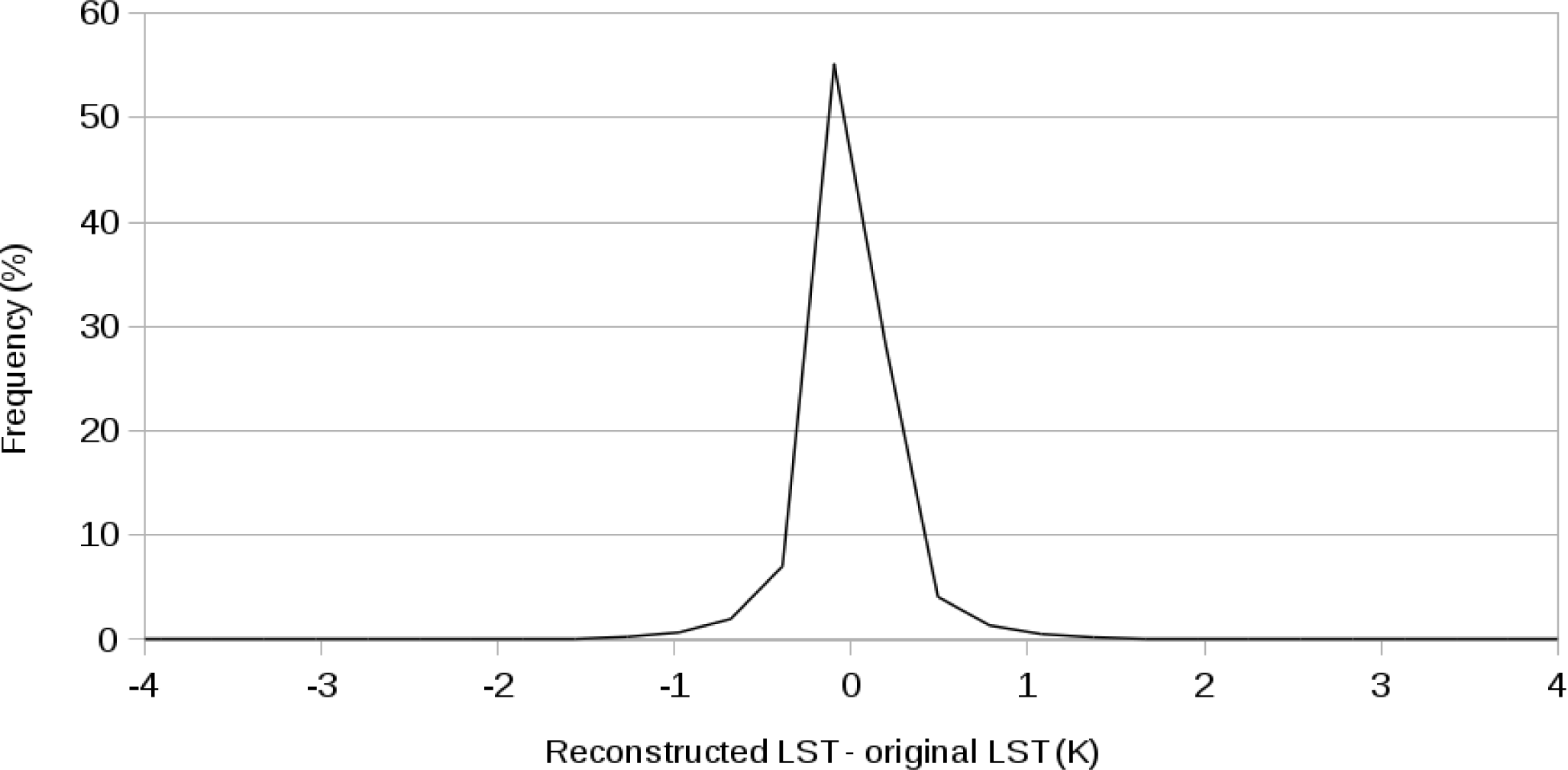
First, we compared original and reconstructed MODIS LST values for twelve days both in the year 2003 and in the year 2010. This test would only compare pixels for which original values exist and is thus not a test for the gap filling procedure but rather for the introduced spatial enhancement. We expected differences between the original and reconstructed LST values due to the increased spatial resolution, but the differences should not exceed the accuracy specification of the original MODIS product. The absolute of the mean difference was usually below 0.1 K and never larger than 0.4 K, thus below the reported accuracy of 1 K for the MODIS LST products. Furthermore, the standard deviation of the differences was usually below 1 K with a maximum of 2.2 K. The differences between reconstructed and original LST values were considerably smaller than those reported by Crosson et al. [17] in a similar validation test. Inspection of the histograms of the differences did not reveal any bias (see Figure 5 for an example).
Second, we evaluated the performance of the actual gap filling procedure. For this test, we masked out original values, performed the reconstruction procedure and then compared the original with the reconstructed values. Here, we expected larger differences between the original and LST values than in the first evaluation test. The absolute of the mean difference was usually below 0.1 K, with a maximum of 1.41 K. The standard deviation of the differences was larger than in the first validation test, ranging from 1.5 to 4.5 K.
4. Discussion
4.1. Example Applications of the Reconstructed Daily MODIS LST Dataset
The reconstructed MODIS LST dataset was initially created in order to estimate habitat suitability in the scope of vector-borne diseases. For example, the tiger mosquito, Aedes albopictus, an efficient vector of various viruses, cannot overwinter in areas with an average January air temperature of less than 0°C and requires at least 500 mm of rainfall per year [5]. We estimated the areas suitable for Ae. albopictus to overwinter within Europe based on January mean temperature in areas with at least 500 mm of rainfall per year (see Figure 6). We rescaled the January mean temperatures, such that −1°C corresponds to zero (totally unsuitable) and 3°C to one (highly suitable). Values between −1°C and 3°C were transformed using a sigmoidal function [5]. None of the previously published approaches is able to provide such a detailed habitat suitability map at the continental scale (see also [33]). Additionally, Ae. albopictus cannot survive 12-h periods below −10°C [6]. Valleys where the mosquito could survive can thus only be identified using temperature data with high temporal and high spatial resolution.
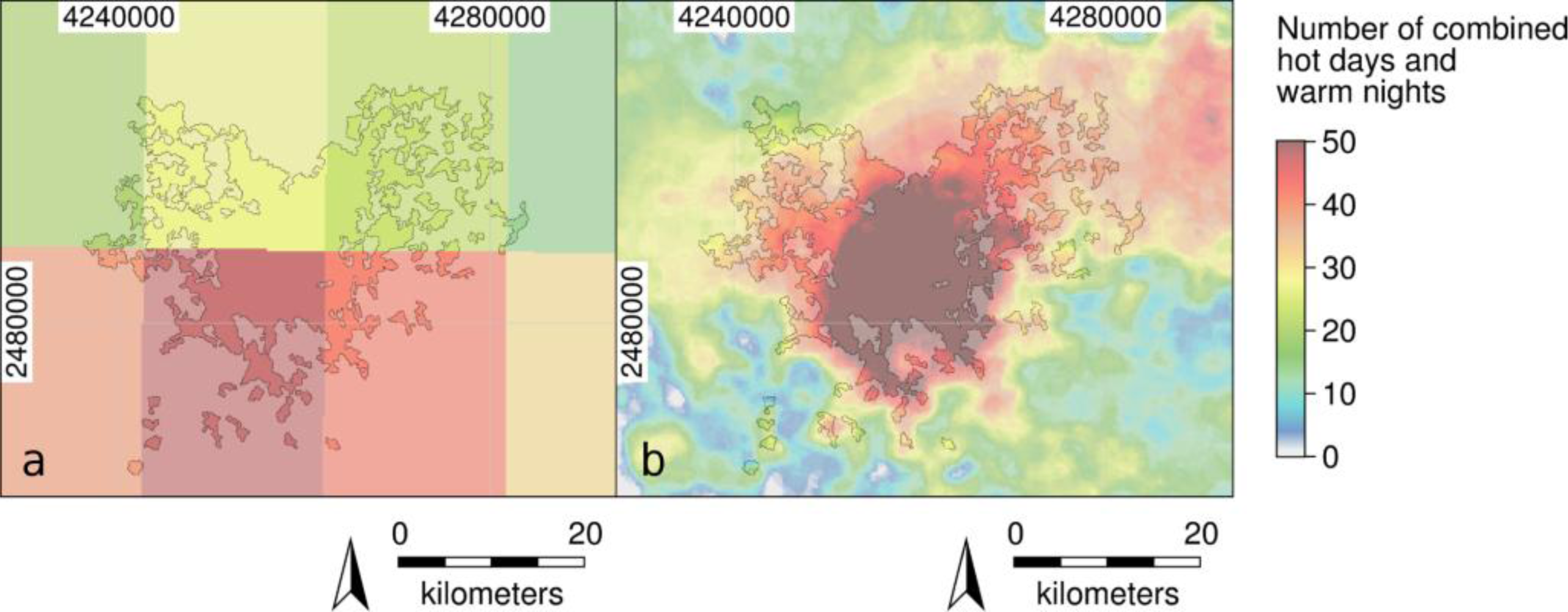
Another example is the identification of urban heat islands (UHIs). UHIs are created by the ongoing urbanization and growth of metropolitan areas, which are significantly warmer than their rural surroundings [34]. The population exposed to UHIs is facing a loss of benefit to or even a severe impact on health. High resolution temperature time series allow decision-makers to identify those UHIs that need to be considered first for mitigation. Figure 7 shows the number of combined hot days (>35 °C) and warm nights (>20 °C; [35]) for the Italian city, Milano, in the year 2003. This analysis requires daily minimum and maximum temperatures. More information on the heat wave risk of European cities is provided by the European Environmental Agency ( http://www.eea.europa.eu/data-and-maps/explore-interactive-maps/heat-wave-risk-of-european-cities-1).
4.2. LST Interpolation and Aggregation
MODIS LST, often together with other auxiliary data, has been regularly used to estimate near-surface air temperature [19–21,36,37]. In these and similar studies, gap-free LST datasets were needed to obtain gap-free near-surface estimates; otherwise, any spatio-temporal gaps in the predictors would also be present in the estimates. Therefore, gaps in the MODIS LST products due to cloud cover must be eliminated to obtain a complete, gap-free time series dataset. A common solution to this problem is to reduce the detail by either using a coarser spatial or a coarser temporal resolution, or both. However, for many applications, weekly or monthly aggregates would be unsuitable, because daily data are required as input, and instead of spatial aggregation, a surface interpolation approach is more appropriate in order to preserve spatial detail. Spatial aggregation combines several pixel values into one new value, whereas gap interpolation estimates missing values by considering the spatial pattern of surrounding valid pixel values. For other applications, the full MODIS LST dataset with four values per day can be easily summarized and aggregated to, e.g., weekly, monthly or seasonal data (see Table 2 for a list of some derivatives and the previous section). LST data from geostationary satellites with a high temporal resolution (that records every few minutes) could be used in a more fine-tuned temporal reconstruction process, because for any given location, the chances are higher to obtain some valid records within a given day. A simple temporal average would in this case be inadequate, because records would come from different times of the day. Geostationary satellites do not provide global coverage, thus an individual procedure would need to be established for each geostationary satellite.
4.3. Potential Error Sources
As with other LST reconstruction approaches (e.g., [13,17]), the reconstructed LST dataset assumes clear-sky conditions or intermittent cloudiness. With intermittent cloudiness, the surface temperature will still be lower than under persistently cloud-free conditions, but LST reconstructed from remote sensing data will always be an overestimate for areas under persistent cloud cover. The accuracy of LST reconstruction could be improved by including additional data sources, such as emissivity-dependent models on LST dynamics. We regard persistent cloud cover as the main source of inaccuracy in the reconstructed LST values. Another source of inaccuracy is the spatial interpolation using splines. The b-spline approach used here prevents overshoots (excessively high or low values), but at the same time, might smooth out local extremes. The same principle holds true for temporal averaging: if there is an extreme event, but no original LST value is available, this extreme event cannot be estimated from the previous and following days. We assume that hot and cold spells typically last for several days, which increases the chances that these events are at least represented in the original LST values. Lastly, we rely on the quality assessment included in the MODIS products. Any errors in the quality assessment where bad quality pixels are erroneously flagged as good quality pixels would be directly reflected in both the original and the reconstructed LST values.
4.4. Spatial and Temporal Resolution
The spatial resolution can significantly affect the results for certain applications, e.g., disease risk assessment or mapping heat waves in urban areas. With too coarse of a resolution, high risk areas can remain undetected, the spatial equivalent of a statistical Type II error, as previously shown in Figure 4, illustrating the heat wave in Europe in July 2003, using station data (CRU TS and ECA&D) and our enhanced MODIS LST. The general pattern on the continental scale is similar, but only the high resolution of MODIS is able to detect hot areas in valleys, causing false negatives (undetected hot areas) in the two other datasets.
The ability of temperature-based suitability maps to identify small islands of high suitability is directly dependent on the spatial resolution. Such “islands” cannot be identified with too coarse of a resolution in areas with high temperature variability, e.g., mountainous areas with a resolution of 10 km or coarser, where valleys narrower than the grid resolution and risk areas smaller than the pixel size cannot be represented by the data. High spatial temperature variability is not only present in topologically complex terrain (Figure 6), but can also be observed in flat areas, e.g., due to differences in land cover and land use (Figure 7).
We regard a detailed temperature time series dataset to be relevant for a series of other applications. Temperature time series are required for risk assessments of fast spreading agricultural pests, e.g., Drosophila suzukii, when using environmental indicators relevant for the respective species lifecycle. Agricultural suitability analyses, e.g., for grapevine varieties [38], rely on temperature time series. Studies of the consequences of the ongoing climate change, e.g., recent extreme temperature anomalies [39], are based on temperature time series, as well as investigations of the impact of global warming on local ecosystems in more detail [8,39]. Heat wave monitoring detects unusually high peaks in temperature time series. As a prominent example, the heat wave of summer, 2003 (Europe), is clearly visible from space at high spatial resolution (Figures 4 and 7). Late frost events in spring may have a significant damaging impact on plants and lead to an economic loss in agriculture [40]. Additionally, late frost is considered to be an abiotic factor triggering tree mast [41], which, in turn, leads to high rodent densities and, subsequently, to Hantavirus epidemics, as observed in temperate Europe [42].
Furthermore, our proposed reconstruction method can be adapted for RS-derived LST time series other than the MODIS LST products. For example, the GlobTemperature initiative of the European Space Agency (ESA), which is also aware of the need to fill gaps due to cloud cover, intends to create an LST time series database by merging data from different sensors. These data, being remotely sensed data, also contain gaps in space and time that need to be filled in order to create a seamless and gap-free database.
5. Dataset Availability
Due to the sheer size of the full dataset (13 TB), we offer aggregated reconstructed MODIS LST data (see the list in Table 2) to scientists and practitioners for free download in common GIS formats ( http://gis.cri.fmach.it/eurolst/).
6. Conclusions
To our knowledge, this is the first attempt to fully reconstruct climatic data acquired with remote sensing at high spatial and temporal detail with a continental extent covering very different climatic zones, while enhancing spatial detail. Concerning scale, there is, in general, an inverse relation between grain (sensu Dungan et al. [43]) and extent: modeling approaches are preferably applied at the local scale with higher resolution data or at the global scale with lower resolution data. Our approach is one of the few examples applying intensive data processing on a large spatial extent with both high spatial and temporal resolution data. The public availability of MODIS LST data together with the free and open source software used (MRT, GRASS GIS) guarantees a high reproducibility of our approach, also allowing peer review of the code used [31]. We believe that this new reconstruction method has the potential to produce results with hitherto unprecedented detail and accuracy in various fields, e.g., agriculture, environmental monitoring, epidemiology and mapping of temperature anomalies.
Supplementary Data
remotesensing-06-03822-s001.pdfAcknowledgments
We are grateful to the NASA Land Processes Distributed Active Archive Center (LP DAAC) for making the MODIS LST data available. We acknowledge the Earth observation E-OBS dataset from the EU-FP6 project ENSEMBLES ( http://ensembles-eu.metoffice.com) and the data providers in the ECA&D project ( http://www.ecad.eu). We are grateful to CERN and Fermilab for providing Scientific Linux. We thank Mirjam Knörnschild, Sajid Pareeth and Luigi Ponti for helpful reviews that significantly improved the paper. We thank Luca Delucchi for assistance in data management and Antonio Galea and Paolo Lenti for invaluable technical support on the HPC environment.
Author Contribution
MM and MN developed the methodology and performed the analysis. MM, DR, and MN wrote the manuscript.
Conflict of Interest
The authors declare no conflict of interest.
References
- Hall, A.; Louis, J.; Lamb, D. Characterising and mapping vineyard canopy using high-spatial-resolution aerial multispectral images. Comput. Geosci 2003, 29, 813–822. [Google Scholar]
- Arnó, J.; Martínez Casasnovas, J.A.; Ribes Dasi, M.; Rosell, J.R. Review. Precision viticulture. Research topics, challenges and opportunities in site-specific vineyard management. Span. J. Agric. Res 2009, 7, 779–790. [Google Scholar]
- Albright, T.P.; Pidgeon, A.M.; Rittenhouse, C.D.; Clayton, M.K.; Wardlow, B.D.; Flather, C.H.; Culbert, P.D.; Radeloff, V.C. Combined effects of heat waves and droughts on avian communities across the conterminous United States. Ecosphere 2010, 1. doi: org/10.1890/ES10-00057.1. [Google Scholar]
- Neteler, M.; Roiz, D.; Rocchini, D.; Castellani, C.; Rizzoli, A. Terra and Aqua satellites track tiger mosquito invasion: Modeling the potential distribution of Aedes albopictus in north-eastern Italy. Int. J. Health Geogr 2011, 10. [Google Scholar] [CrossRef]
- Caminade, C.; Medlock, J.M.; Ducheyne, E.; McIntyre, K.M.; Leach, S.; Baylis, M.; Morse, A.P. Suitability of European climate for the Asian tiger mosquito Aedes albopictus: Recent trends and future scenarios. J. R. Soc. Interface 2012, 9, 2708–2717. [Google Scholar]
- Thomas, S.M.; Obermayr, U.; Fischer, D.; Kreyling, J.; Beierkuhnlein, C. Low-temperature threshold for egg survival of a post-diapause and non-diapause European aedine strain, Aedes albopictus (Diptera: Culicidae). Parasit. Vectors 2012, 5. [Google Scholar] [CrossRef]
- Tomlinson, C.J.; Chapman, L.; Thornes, J.E.; Baker, C. Remote sensing land surface temperature for meteorology and climatology: A review. Meteorol. Appl 2011, 18, 296–306. [Google Scholar]
- Walther, G.-R.; Post, E.; Convey, P.; Menzel, A.; Parmesan, C.; Beebee, T.J. C.; Fromentin, J.-M.; Hoegh-Guldberg, O.; Bairlein, F. Ecological responses to recent climate change. Nature 2002, 416, 389–395. [Google Scholar]
- Wan, Z. New refinements and validation of the MODIS Land-Surface Temperature/Emissivity products. Remote Sens. Environ 2008, 112, 59–74. [Google Scholar]
- Viña, A.; Bearer, S.; Zhang, H.; Ouyang, Z.; Liu, J. Evaluating MODIS data for mapping wildlife habitat distribution. Remote Sens. Environ 2008, 112, 2160–2169. [Google Scholar]
- Coops, N.C.; Wulder, M.A.; Iwanicka, D. Demonstration of a satellite-based index to monitor habitat at continental-scales. Ecol. Indic 2009, 9, 948–958. [Google Scholar]
- Sulla-Menashe, D.; Friedl, M.A.; Krankina, O.N.; Baccini, A.; Woodcock, C.E.; Sibley, A.; Sun, G.; Kharuk, V.; Elsakov, V. Hierarchical mapping of Northern Eurasian land cover using MODIS data. Remote Sens. Environ 2011, 115, 392–403. [Google Scholar]
- Neteler, M. Estimating daily Land Surface Temperatures in mountainous environments by reconstructed MODIS LST data. Remote Sens 2010, 2, 333–351. [Google Scholar]
- Scharlemann, J.P.; Benz, D.; Hay, S.I.; Purse, B.V.; Tatem, A.J.; Wint, G.R.; Rogers, D.J. Global data for ecology and epidemiology: A novel algorithm for temporal Fourier processing MODIS data. PLoS One 2008, 3. [Google Scholar] [CrossRef]
- Jönsson, P.; Eklundh, L. Seasonality extraction by function fitting to time-series of satellite sensor data. IEEE Trans. Geosci. Remote Sens 2002, 40, 1824–1832. [Google Scholar]
- Coops, N.C.; Duro, D.C.; Wulder, M.A.; Han, T. Estimating afternoon MODIS land surface temperatures (LST) based on morning MODIS overpass, location and elevation information. Int. J. Remote Sens 2007, 28, 2391–2396. [Google Scholar]
- Crosson, W.L.; Al-Hamdan, M.Z.; Hemmings, S.N.J.; Wade, G.M. A daily merged MODIS Aqua–Terra land surface temperature data set for the conterminous United States. Remote Sens. Environ 2012, 119, 315–324. [Google Scholar]
- Roerink, G.J.; Menenti, M.; Verhoef, W. Reconstructing cloudfree NDVI composites using Fourier analysis of time series. Int. J. Remote Sens 2000, 21, 1911–1917. [Google Scholar]
- Hengl, T.; Heuvelink, G.B.M.; Perčec Tadić, M.; Pebesma, E.J. Spatio-temporal prediction of daily temperatures using time-series of MODIS LST images. Theor. Appl. Climatol 2011, 107, 265–277. [Google Scholar]
- Lin, S.; Moore, N.J.; Messina, J.P.; DeVisser, M.H.; Wu, J. Evaluation of estimating daily maximum and minimum air temperature with MODIS data in east Africa. Int. J. Appl. Earth Obs. Geoinf 2012, 18, 128–140. [Google Scholar]
- Benali, A.; Carvalho, A.C.; Nunes, J.P.; Carvalhais, N.; Santos, A. Estimating air surface temperature in Portugal using MODIS LST data. Remote Sens. Environ 2012, 124, 108–121. [Google Scholar]
- Pasotti, L.; Maroli, M.; Giannetto, S.; Brianti, E. Agrometeorology and models for the parasite cycle forecast. Parassitologia 2006, 48, 81–83. [Google Scholar]
- Cini, A.; Ioriatti, C.; Anfora, G. A review of the invasion of Drosophila suzukii in Europe and a draft research agenda for integrated pest management. Bull. Insectol 2012, 65, 149–160. [Google Scholar]
- Haylock, M.R.; Hofstra, N.; Tank, A.M.G.K.; Klok, E.J.; Jones, P.D.; New, M. A European daily high-resolution gridded data set of surface temperature and precipitation for 1950–2006. J. Geophys. Res 2008, 113. [Google Scholar] [CrossRef]
- Mitchell, T.D.; Jones, P.D. An improved method of constructing a database of monthly climate observations and associated high-resolution grids. Int. J. Climatol 2005, 25, 693–712. [Google Scholar]
- Reda, I.; Andreas, A. Solar position algorithm for solar radiation applications. Solar Energy 2004, 76, 577–589. [Google Scholar]
- Rolland, C. Spatial and seasonal variations of air temperature lapse rates in Alpine Regions. J. Clim 2003, 16, 1032–1046. [Google Scholar]
- Brovelli, M.A.; Cannata, M.; Longoni, U.M. LIDAR data filtering and DTM interpolation within GRASS. Trans. GIS 2004, 8, 155–174. [Google Scholar]
- Hengl, T.; Heuvelink, G.; Rossiter, D. About regression-kriging: From equations to case studies. Comput. Geosci 2007, 33, 1301–1315. [Google Scholar]
- Neteler, M.; Bowman, M.H.; Landa, M.; Metz, M. GRASS GIS: A multi-purpose open source GIS. Environ. Model. Softw 2012, 31, 124–130. [Google Scholar]
- Rocchini, D.; Neteler, M. Let the four freedoms paradigm apply to ecology. Trends Ecol. Evol 2012, 27, 310–311. [Google Scholar]
- R Development Core Team. R Development Core Team R: A Language and Environment for Statistical Computing; R Foundation for Statistical Computing: Vienna, Austria, 2009. [Google Scholar]
- Neteler, M.; Metz, M.; Rocchini, D.; Rizzoli, A.; Flacio, E.; Engeler, L.; Guidi, V.; Lüthy, P.; Tonolla, M. Is Switzerland suitable for the invasion of Aedes albopictus? PLoS One 2013, 8. [Google Scholar] [CrossRef]
- Oke, T.R. The energetic basis of the urban heat island. Q. J. R. Meteorol. Soc 1982, 108, 1–24. [Google Scholar]
- Fischer, E.M.; Schär, C. Consistent geographical patterns of changes in high-impact European heatwaves. Nat. Geosci 2010, 3, 398–403. [Google Scholar]
- Hill, D.J. Evaluation of the temporal relationship between daily min/max air and land surface temperature. Int. J. Remote Sens 2013, 34, 9002–9015. [Google Scholar]
- Vancutsem, C.; Ceccato, P.; Dinku, T.; Connor, S. Evaluation of MODIS land surface temperature data to estimate air temperature in different ecosystems over Africa. Remote Sens. Environ 2010, 114, 449–465. [Google Scholar]
- Zorer, R.; Rocchini, D.; Metz, M.; Delucchi, L.; Zottele, F.; Meggio, F.; Neteler, M. Daily MODIS land surface temperature data for the analysis of the heat requirements of Grapevine varieties. IEEE Trans. Geosci. Remote Sens 2013, 51, 2128–2135. [Google Scholar]
- Hansen, J.; Sato, M.; Ruedy, R. Perception of climate change. Proc. Natl. Acad. Sci 2012, 109, E2415–E2423. [Google Scholar]
- Gu, L.; Hanson, P.J.; Post, W.M.; Kaiser, D.P.; Yang, B.; Nemani, R.; Pallardy, S.G.; Meyers, T. The 2007 Eastern US spring freeze: Increased cold damage in a warming world. BioScience 2008, 58, 253–262. [Google Scholar]
- Piovesan, G.; Adams, J.M. Masting behaviour in beech: Linking reproduction and climatic variation. Can. J. Bot 2001, 79, 1039–1047. [Google Scholar]
- Heyman, P.; Thoma, B.R.; Marié, J.-L.; Cochez, C.; Essbauer, S.S. In search for factors that drive hantavirus epidemics. Front. Physiol 2012, 3. [Google Scholar] [CrossRef]
- Dungan, J.; Perry, J.; Dale, M.; Legendre, P.; Citron-Pousty, S.; Fortin, M.; Jakomulska, A.; Miriti, M.; Rosenberg, M. A balanced view of scale in spatial statistical analysis. Ecography 2002, 25, 626–640. [Google Scholar]


| Authors | Method | Spatial Extent | Spatial Resolution | Temporal Extent | Temporal Resolution * | Output |
|---|---|---|---|---|---|---|
| Scharlemann et al., 2008 [14] | Temporal Fourier transform | Global | 1000 m | 2001–2005 | 2 maps/8 days | 34 parameters describing LST temporal cycles |
| Neteler, 2010 [13] | Volumetric (3D) splines | Part of Northern Italy | 200 m | 2000–2008 | 4 maps/day | Fully reconstructed time series |
| Crosson et al., 2012 [17] | Seasonal mean | Conterminous USA | 1000 m | 2003–2008 | 4 maps/day | Partially reconstructed time series |
| Hengl et al., 2011 [19] | Temporal average, 2D splines | Croatia | 1000 m | 2008 | 2 maps/8 days | Fully reconstructed time series |
| Benali et al., 2012 [21] | Temporal aggregation | Portugal | 1000 m | 2000–2009 | 2 maps/day | Partially reconstructed time series |
| Present study | Temporal average, multiple regression, splines | Europe | 250 m | 2000–2013 | 4 maps/day | Fully reconstructed time series |
| Code | Description |
|---|---|
| BIO1 | Annual mean temperature (°C × 10) |
| BIO2 | Mean diurnal range (monthly mean of diurnal range; °C × 10) |
| BIO3 | Isothermality ((BIO2/BIO7) × 100) |
| BIO4 | Temperature seasonality (standard deviation × 100) |
| BIO5 | Maximum temperature of the warmest month (°C × 10) |
| BIO6 | Minimum temperature of the coldest month (°C × 10) |
| BIO7 | Temperature annual range (BIO5–BIO6) (°C × 10) |
| BIO10 | Mean temperature of the warmest quarter (°C × 10) |
| BIO11 | Mean temperature of the coldest quarter (°C × 10) |
| Monthly mean | Monthly mean temperature (°C × 10) |
| Daytime Overpasses | Nighttime Overpasses | |||
|---|---|---|---|---|
| Month | Terra | Aqua | Terra | Aqua |
| January | 15.29% | 13.65% | 20.39% | 18.56% |
| February | 17.33% | 14.86% | 22.27% | 20.63% |
| March | 22.96% | 20.71% | 26.35% | 24.97% |
| April | 28.36% | 25.26% | 29.78% | 29.40% |
| May | 33.45% | 28.81% | 33.86% | 31.68% |
| June | 36.68% | 33.66% | 37.77% | 33.91% |
| July | 40.65% | 35.64% | 42.08% | 34.75% |
| August | 40.42% | 36.35% | 41.66% | 34.60% |
| September | 38.64% | 34.77% | 38.90% | 33.03% |
| October | 29.25% | 26.43% | 27.94% | 24.57% |
| November | 20.55% | 18.41% | 23.52% | 21.03% |
| December | 14.79% | 13.49% | 18.59% | 17.14% |
© 2014 by the authors; licensee MDPI, Basel, Switzerland This article is an open access article distributed under the terms and conditions of the Creative Commons Attribution license (http://creativecommons.org/licenses/by/3.0/).
Share and Cite
Metz, M.; Rocchini, D.; Neteler, M. Surface Temperatures at the Continental Scale: Tracking Changes with Remote Sensing at Unprecedented Detail. Remote Sens. 2014, 6, 3822-3840. https://doi.org/10.3390/rs6053822
Metz M, Rocchini D, Neteler M. Surface Temperatures at the Continental Scale: Tracking Changes with Remote Sensing at Unprecedented Detail. Remote Sensing. 2014; 6(5):3822-3840. https://doi.org/10.3390/rs6053822
Chicago/Turabian StyleMetz, Markus, Duccio Rocchini, and Markus Neteler. 2014. "Surface Temperatures at the Continental Scale: Tracking Changes with Remote Sensing at Unprecedented Detail" Remote Sensing 6, no. 5: 3822-3840. https://doi.org/10.3390/rs6053822