Using InSAR Coherence to Map Stand Age in a Boreal Forest

1
Department of Geographical Sciences, University of Maryland, 2181 LeFrak Hall, College Park, MD 20742, USA
2
Jet Propulsion Laboratory/California Institute of Technology, 4800 Oak Grove Dr., Pasadena, CA 91109, USA
*
Author to whom correspondence should be addressed.
Remote Sens. 2013, 5(1), 42-56; https://doi.org/10.3390/rs5010042
Submission received: 1 October 2012
/
Revised: 27 November 2012
/
Accepted: 28 November 2012
/
Published: 24 December 2012
Abstract
:The interferometric coherence parameter γ estimates the degree of correlation between two Synthetic Aperture Radar (SAR) images and can be influenced by vegetation structure. Here, we investigate the use of repeat-pass interferometric coherence γ to map stand age, an important parameter for the study of carbon stocks and forest regeneration. In August 2009 NASA’s L-band airborne sensor UAVSAR (Uninhabited Aerial Vehicle Synthetic Aperture Radar) acquired zero-baseline data over Quebec with temporal separation ranging between 45 min and 9 days. Our analysis focuses on a 66 km2 managed boreal forest and addresses three questions: (i) Can coherence from L-band systems be used to model forest age? (ii) Are models sensitive to weather events and temporal baseline? and (iii) How is model accuracy impacted by the spatial scale of analysis? Linear regression models with 2-day baseline showed the best results and indicated an inverse relationship between γ and stand age. Model accuracy improved at 5 ha scale (R2 = 0.75, RMSE = 5.3) as compared to 1 ha (R2 = 0.67, RMSE = 5.8). Our results indicate that coherence measurements from L-band repeat-pass systems can estimate forest age accurately and with no saturation. However, empirical model relationships and their accuracy are sensitive to weather events, temporal baseline, and spatial scale of analysis.
1. Introduction
1.1. Motivation
Land use change, in particular carbon uptake from forest regrowth, remains a significant source of uncertainty in the terrestrial carbon budget [1–3] and the contribution of boreal biomes, based on forest inventories, is on the order of 15–25% [3]. Canada ranks second in gross forest cover loss [4] owing to forest fires and insect outbreaks. It has been estimated that Canada’s biomass C sink in managed forests has been reduced by half between 1990–2000 and 2000–2007 [3]. However, such estimates are poorly constrained because of the uncertainty in quantifying fine-scale disturbance and subsequent regrowth, underscoring the need for remote sensing data [5].
In the absence of repeat observation of forest biomass through time, stand age maps can be employed to study forest regeneration. For example, forest age estimates have been used in combination with lidar and field plots to generate yield curves that predict post-disturbance carbon accumulation [6,7]. Stand age can be estimated from dense Landsat time series that reveal the most recent date of forest disturbance [8]. A complementary approach, presented here, is to build empirical models that exploit the relationship between forest structure and age at a given point in time.
Forest age has been modeled from Synthetic Aperture Radar (SAR) backscatter texture [9], but in many cases researchers can only resolve recently disturbed and old growth stands [10,11] and confidence intervals increase with stand age [12]. Backscatter temporal variation has also been used to model stand age [13,14], but this approach requires multiple acquisitions.
Techniques from Interferometric SAR (InSAR) can also provide information on forest structural parameters by combining information from two acquisitions. The interferometric coherence γ[15] is a parameter that measures the similarity between two images and can be estimated from two co-registered SAR images as:
where S1 and S2 are single look complex (SLC) images acquired at times t1 and t2, the star (*) denotes complex conjugation, and angular brackets indicate averaging over a finite number of signal measurements (i.e., taking a sample of pixels).
The coherence parameter γ was originally used to provide a confidence interval for the interferometric phase [16]. Forest stands lead to a decrease in phase coherence (referred to as “decorrelation”), which in turn reduces accuracy of land deformation and terrain elevation retrievals from interferometry. An important implication here is that interferometric coherence is influenced by the distribution of vegetation material and can be exploited to gain insights about forest structure. The objective of this study is to assess a method based on repeat-pass Interferometric Synthetic Aperture Radar (InSAR) coherence to map stand age in a managed forest in Quebec. In the following, we describe the impact of forest structure on coherence and the L-band airborne dataset being used here to derive coherence estimates.
1.2. Modeling Forest Structure from InSAR Coherence Maps
In repeat-pass systems there is a time delay between the two acquisitions, in which case interferometric coherence can be attributed to four main components [17]:
where γN is the correlation due to thermal noise, γG is the geometric or baseline correlation, γZ is the volume correlation, and γT is temporal correlation. Volume decorrelation γZ can be modeled as a function of canopy height and penetration depth [18]. The impact of temporal decorrelation (γT) is significant over forest stands due to movement of scatterers between acquisitions or changes in their dielectric properties. Thus, temporal decorrelation is expected to be strongly dependent on weather events such as wind, precipitation, and snow melt.
Several studies have modeled forest structure from repeat-pass coherence data acquired by the C-band European Remote Sensing satellites (ERS-1/2). Temporal decorrelation has been generally treated as model error [19,20]. A few authors, however, have assessed the structural information present in temporal decorrelation. Askne et al.[18] assumed wind-induced decorrelation related to canopy height, whereas Castel et al.[21] demonstrated the impact of wind on temporal decorrelation was more important in tall, mature forest stands. More recent work with airborne L-band data shows the relationship between temporal decorrelation and land cover [22] as well as canopy height [23,24]. Given these observations and the fact forest structure changes with age, it is conceivable that interferometric coherence could be used to map forest age. The present work covers existing knowledge gaps regarding our ability to map forest age with L-band coherence data. Specifically, our analyses address three questions: (i) Can coherence from L-band systems be used to model forest age? (ii) Are models sensitive to weather events and temporal baseline? and (iii) How is model accuracy impacted by the spatial scale of analysis?
1.3. Remote Sensing Data
We use repeat-pass L-band InSAR data acquired by NASA’s airborne sensor UAVSAR (Uninhabited Aerial Vehicle Synthetic Aperture Radar) [25]. In 2009, UAVSAR acquired repeat-pass data over the Laurentides Wildlife Reserve in the Quebec province [26]. The spatial separation between pairs of flight lines (spatial baseline) was nominally zero, and the temporal separation (temporal baseline) ranged between 45 min and 9 days. Our analyses are restricted to Montmorency Forest, a 66 km2 managed boreal forest with stands ranging between 2–42 years. Given UAVSAR observation parameters and zero nominal baseline, the impacts of γG, γZ, and γN are negligible and decorrelation is mainly due its temporal component γT[24]. This experiment has thus allowed us to focus on and exploit the impacts of temporal decorrelation on forest age mapping. We additionally used lidar data from the Laser Vegetation Imaging Sensor (LVIS) [27] to characterize forest structure across age classes. LVIS flew over the Laurentides Reserve in August 2009 and acquired two tracks with 2.8 km swath. Canopy profiles from LVIS waveforms are strongly influenced by forest successional stage [28]. In this paper, we do not attempt to optimize the use of LVIS data to obtain stand age. Instead, the LVIS waveform quantile metrics serve to characterize basic structural differences across forest age classes that may impact InSAR coherence, which is the main focus of this paper.
2. Methods
2.1. Study Site
Our study area is Montmorency Forest, located 80 km north of Quebec City and adjacent to the Laurentides Wildlife Reserve (Figure 1). The forest is part of a post-glacial ecosystem with elevation ranging between 500 and 1,000 m. Montmorency lies at the Northern limit of the temperate seasonal forest biome [29]. The average daily temperature is 9.8 °C in May–October and −9.2 °C in November–April [30]. Forest composition however is typical of the boreal mixed wood zone [31,32]. Owing to infrequent fire disturbances the forest dynamics are largely controlled by periodic epidemics of spruce budworm and windthrow [33]. As a result the tree community is dominated by Balsam fir (Abies Balsamea), but also includes White spruce (Picea Glauca), Black spruce (Picea Mariana), and Paper birch (Betula Paryrifera) [34].
Since 1964, Université Laval manages Montmorency Forest to ensure that the size/frequency of cuts is compatible with the historical disturbances for this site [34]. The resulting landscape is a mosaic of forest successional stages, with even-aged patches ranging between 0.5 and 100 ha and approximately equal contribution of early growth (0–20 years), late secondary (20–40 years), and late successional (>40 years) patches. Most of the forest regrowth follows natural regeneration [34]. Water accumulation on the soil surface is high in Montmorency due to its dense cover with >50 species of mosses and lichens [35].
2.2. UAVSAR Correlation and Backscatter
UAVSAR acquired data over the Laurentides Wildlife Reserve (Figure 1) during the leaf-on period in August 2009. We processed 5 pairs of co-registered images with zero nominal spatial baseline and temporal baselines ranging between 45 min and 9 days (Table 1). Interferometric coherence was computed from the slant-range SLC images using Equation (1) and a sample size of 10 × 5 pixels in range and azimuth direction, respectively. Results were geocoded to produce ground range images with 5 m resolution.
In order to compare UAVSAR coherence measurements with more widely used backscatter data, we also processed the SLC images acquired on 5August and7 August (Table 1) to generate terrain calibrated and radiometrically normalized backscatter images (γ°) for channels HH, HV, and VV.
2.3. Weather Data
We expect temporal changes to be encompassed by movement of large branches and variation in vegetation and soil moisture following weather events. For this reason we report rainfall and wind speed measurements for a weather station in Montmorency (available through Canada’s National Climate Data and Information Archive, http://www.climate.weatheroffice.gc.ca). We also set one weather station and five rain gauges along Highway 175, at a distance between 18–60 km from Montmorency Forest. Rain gauges were checked and emptied in the mornings between 3 August and 14 August.
Our field site received substantial rainfall on 4, 7, 9, and 10 August (Figure 2) and the UAVSAR images acquired during the 7 August flight were most likely impacted by wet vegetation and wind. Our weather stations indicate that most of the rainfall took place in the morning of 7 August, before the UAVSAR flight at 16:15.
2.4. Canopy Height and Height Metrics
LVIS data were processed to produce 25 m resolution gridded maps. Our analyses included widely used waveform percentile metrics that correlate with top canopy height (RH100) [36], basal area weighted canopy height (RH75) [37], and aboveground biomass (RH50) [28,38]. In addition we used the ratio RH50/RH100 to enhance variations in vertical distribution of vegetation material relative to top canopy height RH100. The waveform percentile metrics are calculated using the % energy accumulated starting at the ground peak (e.g., RH75 is the height in meters where we find 75% of cumulative energy).
2.5. GIS and Statistical Analyses
Patch location and age (number of years since the last cut) were obtained from Université Laval’s Montmorency Forest, in a GIS shapefile format containing polygons representing forest stands. We found cases in which disjoint patches were given the same identification code, as well as adjacent patches that had the same age but different identification codes. These issues were addressed in a GIS environment to ensure that disjoint patches served as our units of analyses. The data processing consisted of performing a “dissolve features” followed by an “explode features” operation on the original shapefile in ArcGIS (ESRI, Redlands, CA, USA). Following this procedure we obtained a total of 459 patches. The amount of overlap (in ha) between forest patches and UAVSAR/LVIS grids was then calculated. The resulting area depended on patch size, but also on patch position with respect to the UAVSAR and LVIS swaths.
Patch-level statistics were derived [21] for both lidar and coherence measurements. We set two thresholds in patch area: 1 ha, matching the area at which forest carbon stocks are usually reported, and 5 ha, to explore a possible model improvement due to averaging more pixels [39]. For each patch, we computed the mean and variance of RH100, RH75, RH50, calibrated backscatter (γ°) for channels HH, HV, and HH, as well as interferometric coherence (γ) for each temporal baseline (Table 1). All statistics were weighted to account for the proportion (%) of each pixel overlapping with its corresponding patch. The extracted values were then used as part of a linear regression to model patch age as a function of radar measurements. We report results for both ordinary least squares regression and robust regression [40].
3. Results
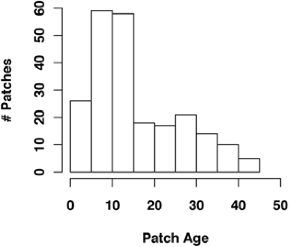
Mean patch age was 15 ± 10 years (Figure 3). Montmorency Forest was almost entirely covered by the UAVSAR track but only partially covered by the LVIS track (Figure 1), therefore models including LVIS metrics include fewer samples. For the UAVSAR track, we found 84 patches with >5 ha overlap and 228 patches with >1 ha overlap. In the case of the LVIS track, these numbers drop to 70 (>5 ha) and 149 (>1 ha). We selected patches using the 1 ha and 5 ha area thresholds to model patch age from radar and lidar metrics at 5 ha (Table 2) and 1 ha (Table 3).
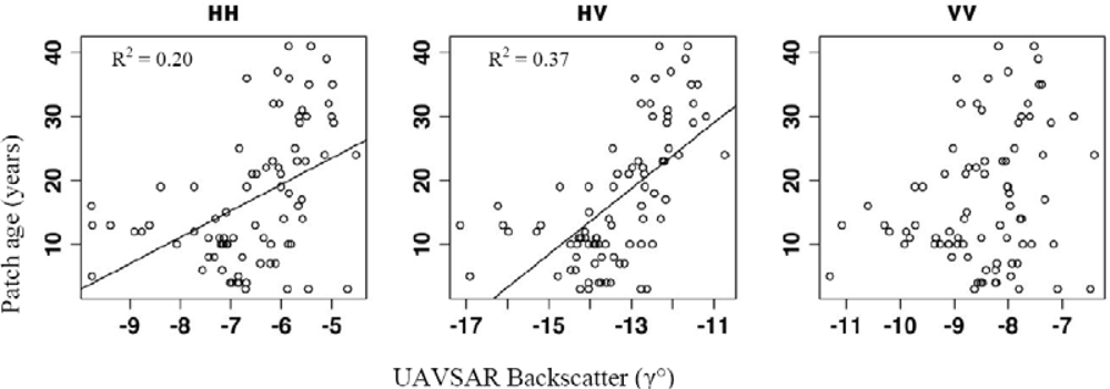
Stand age showed a significant correlation with all lidar-derived structural metrics except for top canopy height (RH100). The best fit was obtained with 5 ha models (Figure 4(A); Tables 2 and 3). We have computed the within-patch standard deviation in RH100 values, and results show significantly more variability in young patches (Figure 4(B)). We also detected a significant linear correlation between stand age and calibrated UAVSAR backscatter at channels HH and HV (Figure 5), and observed no saturation of the SAR signal with stand age. The best result was again found for the 5 ha scale (Tables 2 and 3). Overall, despite the partial overlap with forest patches, LVIS metrics showed better relationship with stand age (best R2 = 0.51; Table 2) as compared to UAVSAR backscatter (best R2 = 0.37; Table 2).
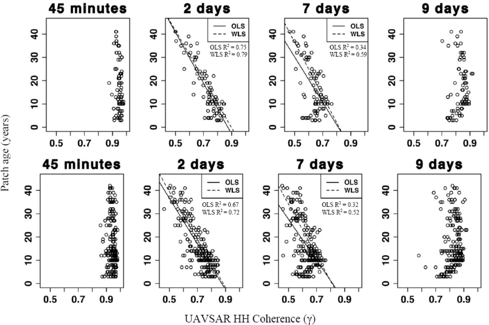
UAVSAR coherence decreased with stand age for both 2-day and 7-day UAVSAR pairs (Figure 6). The best fit of the Ordinary Least Squares (OLS) model used the 2-day pair and improved at the 5 ha scale (R2 = 0.75; RMSE = 5.3 years; Table 2) as compared to 1 ha (R2 = 0.67; RMSE = 8.6 years; Table 3). In contrast, the 45-min and 9-day temporal baselines exhibited a narrow dynamic range of coherence values and no variation across age classes was observed (Figure 6). Both 45-min pairs (Table 1) performed poorly as predictors of stand age so we only show results for the August 7th pair, which had the largest dynamic range of all pairs (Figure 6). Regarding significant models, we found that models with HH coherence pairs had a better fit as compared to HV coherence pairs, with a difference in R2 of about 0.2 (not shown), so all results on Tables 2 and 3 are for the HH channel.
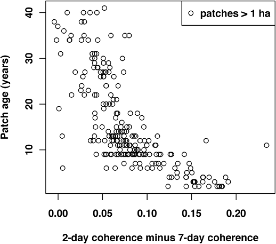
The amount of decorrelation varied greatly with temporal baseline. A more marked difference in decorrelation of the InSAR signal was observed in young forest stands as the temporal baseline increased from 2 to 7 days (Figure 7). To examine this issue, we performed a Weighed Least Squares (WLS) model that weighed each data point by its corresponding age, thereby putting an emphasis on old growth forests. This was performed for all coherence pairs. The main outcome was an increase in the model fit for the 7-day pair (R2 = 0.52 at 1 ha; R2 = 0.59 at 5 ha) at the expense of a ∼20-year increase in the overall model RMSE (Tables 2 and 3).
4. Discussion
We found a linear decrease in UAVSAR interferometric coherence with patch age in Quebec. The best predictions were obtained using the HH channel and averaging coherence data at 5 ha scale (Table 3). In the case of backscatter, we observed a linear increase with stand age and no saturation as previously found with aboveground biomass in other boreal sites [41,42]. However, stand age showed a tighter relationship with InSAR coherence, as has been previously found for C-band studies [20]. In the absence of ground measurements it is not yet possible to ascertain which structural components are changing with respect with forest structure. But based on lidar metrics (Figure 4(A)) it is reasonable to infer that mature patches are associated with taller canopies. The lidar-derived canopy height metric RH100 shows considerable within-patch variation (Figure 4(B)). A stronger correlation with age is observed with RH75 (Table 2), a metric generally associated with basal area-weighted height [37].
Our results agree with past studies that have described a relationship between temporal decorrelation and forest height [23]. In addition, coherence maps from C-band ERS-1/2 including both volume and temporal decorrelation show a relationship with aboveground biomass [21,43] and stem volume [39,44]. Since our experiment employs a zero spatial baseline we can better examine the impacts of temporal decorrelation, in particular the interaction between weather events and forest structure on model fits.
The dynamic range of coherence was small for the 45-min and the 9-days baselines (Figure 6) and failed to generate any spatial patterns (Figure 1). Two 45-min pairs were analyzed in our study. On 7 August, both images were acquired under wet conditions, on 14 August both images were acquired under dry conditions (Figure 2), and both images from the 9-days pair were acquired under dry conditions. We recorded a rainfall event on 7 August but this event is not likely to influence the 9-days pair as it occurred after the first acquisition and one week before the second acquisition. Thus the changes in moisture conditions between acquisitions can be as important in determining temporal decorrelation as the temporal baseline itself. At the same time, we observed wind gusts of up to 40 km/h during acquisitions (Figure 2), but these events were not helpful in resolving forest age at 45-min and 9-days intervals.
Coherence maps using the two intermediate baselines (2 and 7 days) showed variation across forest age classes and produced significant models (Tables 2 and 3). Mature forest patches showed lower coherence in the 2-day pair, suggesting a role for the movement of large branches in old growth forests. Indeed, studies with C-band ERS-1/2 over pine stands show that wind exposure decorrelates the signal over mature patches, but not young patches [21]. It is likely that the top components of tall fir trees are less flexible and more likely to move with wind. At 7 days, we observed the opposite pattern: the UAVSAR signal over young forests showed low coherence values (Figure 7) causing a reduction in the model fit (Figure 6). Our weather stations recorded a rainfall event on 7 August. This suggests a role of soil moisture leading to changes in the soil dielectric properties between acquisitions, thereby contributing to signal decorrelation. Rainfall events are more likely to impact the coherence in young patches with more ground exposure.
5. Conclusions
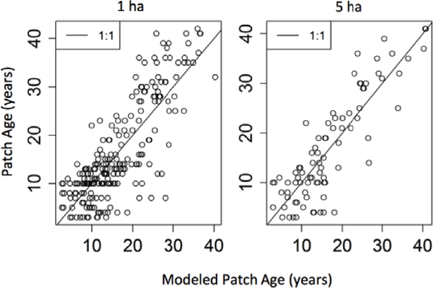
This paper demonstrates the utility of InSAR coherence images in complementing and constraining existing approaches to model forest structure. This is in agreement with recent efforts to map forest stem volume with L-band coherence data [45]. In particular, the empirical models developed here (Figure 6) suggest the possibility of looking beyond the Landsat record to characterize > 30 years old stands, thereby complementing forest disturbance maps from Landsat time series [8]. Our models were strongly dependent on resolution and temporal baseline.
In the best case scenario, that is, the largest observed range of temporal decorrelation (2-days baseline in our case), the model RMSE was 5.8 years, and results improved by aggregating coherence values at 5 ha (Figure 8). Thus, the approach presented here is more useful in areas with large forest stands (as opposed to small forest gaps) and with considerable variation in forest age. At the same time, our results suggest that wind and soil moisture also impacted the model fit, suggesting that temporal decorrelation of the InSAR signal over forest depends on weather events and cannot be inferred based on temporal baseline alone [26]. It is also important to note that the UAVSAR flights planned for this study had zero nominal spatial baseline. If finite spatial baselines are used, empirical models will have to account for the impact of volume decorrelation (Equation (2)).
Acknowledgments
The authors would like to thank Scott Hensley and Yang Zheng for assistance with UAVSAR data, and Matthew Brolly for comments on the manuscript. We are grateful for the GIS dataset for Montmorency provided by Forêt Montmorency, Faculté de Foresterie, de Géographie et de Géomatique de l’Université Laval. M Simard was funded by NASA’s Terrestrial Ecology program (WBS 281945.02.61.01.69). Part of this research was carried out at the Jet Propulsion Laboratory, California Institute of Technology, and was sponsored by the National Aeronautics and Space Administration. Lidar datasets were provided by the Laser Vegetation Imaging Sensor (LVIS) team in the Laser Remote Sensing Branch at NASA Goddard Space Flight Center with support from the University of Maryland, College Park.
References
- Canadell, J.G.; Le Quere, C.; Raupach, M.R.; Field, C.B.; Buitenhuis, E.T.; Ciais, P.; Conway, T.J.; Gillett, N.P.; Houghton, R.A.; Marland, G. Contributions to accelerating atmospheric CO2 growth from economic activity, carbon intensity, and efficiency of natural sinks. Proc. Natl. Acad. Sci. USA 2007, 104, 18866–18870. [Google Scholar]
- Le Quere, C.; Raupach, M.R.; Canadell, J.G.; Marland, G.; Bopp, L.; Ciais, P.; Conway, T.J.; Doney, S.C.; Feely, R.A.; Foster, P.; et al. Trends in the sources and sinks of carbon dioxide. Nat. Geosci 2009, 2, 831–836. [Google Scholar]
- Pan, Y.; Birdsey, R.A.; Fang, J.; Houghton, R.; Kauppi, P.E.; Kurz, W.A.; Phillips, O.L.; Shvidenko, A.; Lewis, S.L.; Canadell, J.G.; et al. A large and persistent carbon sink in the world’s forests. Science 2011, 333, 988–993. [Google Scholar]
- Hansen, M.C.; Stehman, S.V.; Potapov, P.V. Quantification of global gross forest cover loss. PNAS 2010, 107, 8650–8655. [Google Scholar]
- Houghton, R.A. Why are estimates of the terrestrial carbon balance so different? Glob. Change Biol 2003, 9, 500–509. [Google Scholar]
- Dolan, K.; Masek, J.G.; Huang, C.; Sun, G. Regional forest growth rates measured by combining ICESat GLAS and Landsat data. J. Geophys. Res.-Biogeosci. 2009. [Google Scholar] [CrossRef]
- Li, A.; Huang, C.; Sun, G.; Shi, H.; Toney, C.; Zhu, Z.; Rollins, M.G.; Goward, S.N.; Masek, J.G. Modeling the height of young forests regenerating from recent disturbances in Mississippi using Landsat and ICESat data. Remote Sens. Environ 2011, 115, 1837–1849. [Google Scholar]
- Huang, C.; Coward, S.N.; Masek, J.G.; Thomas, N.; Zhu, Z.; Vogelmann, J.E. An automated approach for reconstructing recent forest disturbance history using dense Landsat time series stacks. Remote Sens. Environ 2010, 114, 183–198. [Google Scholar]
- Champion, I.; Dubois-Fernandez, P.; Guyon, D.; Cottrel, M. Radar image texture as a function of forest stand age. Int. J. Remote Sens 2008, 29, 1795–1800. [Google Scholar]
- Kuplich, T.M. Classifying regenerating forest stages in Amazonia using remotely sensed images and a neural network. Forest Ecol. Manage 2006, 234, 1–9. [Google Scholar]
- Luckman, A.J.; Frery, A.C.; Yanasse, C.C.F.; Groom, G.B. Texture in airborne SAR imagery of tropical forest and its relationship to forest regeneration stage. Int. J. Remote Sens 1997, 18, 1333–1349. [Google Scholar]
- McNeill, S.; Pairman, D. Stand age retrieval in production forest stands in New Zealand using C-and L-band polarimetric radar. IEEE Trans. Geosci. Remote Sens 2005, 43, 2503–2515. [Google Scholar]
- Salas, W.A.; Ducey, M.J.; Rignot, E.; Skole, D. Assessment of JERS-1 SAR for monitoring secondary vegetation in Amazonia: I. Spatial and temporal variability in backscatter across a chrono-sequence of secondary vegetation stands in Rondonia. Int. J. Remote Sens 2002, 23, 1357–1379. [Google Scholar]
- Quegan, S.; Le Toan, T.; Yu, J.J.; Ribbes, F.; Floury, N. Multitemporal ERS SAR analysis applied to forest mapping. IEEE Trans. Geosci. Remote Sens 2000, 38, 741–753. [Google Scholar]
- Rosen, P.A.; Hensley, S.; Joughin, I.R.; Li, F.K.; Madsen, S.N.; Rodriguez, E.; Goldstein, R.M. Synthetic aperture radar interferometry. Proc. IEEE 2000, 88, 333–382. [Google Scholar]
- Zebker, H.A.; Werner, C.L.; Rosen, P.A.; Hensley, S. Accuracy of topographic maps derived from Ers-1 Interferometric Radar. IEEE Trans. Geosci. Remote Sens 1994, 32, 823–836. [Google Scholar]
- Zebker, H.A.; Villasenor, J. Decorrelation in interferometric radar echoes. IEEE Trans. Geosci. Remote Sens 1992, 30, 950–959. [Google Scholar]
- Askne, J.I.H.; Dammert, P.B.G; Ulander, L.M.H.; Smith, G. C-band repeat-pass interferometric SAR observations of the forest. IEEE Trans. Geosci. Remote Sens 1997, 35, 25–35. [Google Scholar]
- Santoro, M.; Askne, J.; Smith, G.; Fransson, J.E.S. Stem volume retrieval in boreal forests from ERS-1/2 interferometry. Remote Sens. Environ 2002, 81, 19–35. [Google Scholar]
- Askne, J.; Santoro, M.; Smith, G; Fransson, J.E.S. Multitemporal repeat-pass SAR interferometry of boreal forests. IEEE Trans. Geos. Remote Sens 2003, 41, 1540–1550. [Google Scholar]
- Castel, T.; Martinez, J.M.; Beaudoin, A.; Wegmuller, U.; Strozzi, T. ERS INSAR data for remote sensing hilly forested areas. Remote Sens. Environ 2000, 73, 73–86. [Google Scholar]
- Ahmed, R.; Siqueira, P.; Hensley, S.; Chapman, B.; Bergen, K. A survey of temporal decorrelation from spaceborne L-band repeat-pass InSAR. Remote Sens. Environ 2011, 115, 2887–2896. [Google Scholar]
- Lavalle, M.; Simard, M.; Hensley, S. A temporal decorrelation model for polarimetric radar interferometers. IEEE Trans. Geosci. Remote Sens 2012, 50, 2880–2888. [Google Scholar]
- Simard, M.; Hensley, S.; Lavalle, M.; Dubayah, R.; Pinto, N.; Hofton, M. An empirical assessment of temporal decorrelation using the Uninhabited Aerial Vehicle Synthetic Aperture Radar over forested landscapes. Remote Sens 2012, 4, 975–986. [Google Scholar]
- Hensley, S.; Lou, Y.; Rosen, P.; Wheeler, K.; Zebker, H.; Madsen, S.; Miller, T.; Hoffman, J.; Farra, D. An L-Band SAR for Repeat Pass Deformation Measurements on a UAV Platform. Proceedings of 2nd AIAA Unmanned-Unlimited System, Technologies and Operating-Aerospace, Land and Sea Conference and Workshop and Exhibit, San Diego, CA, USA, 20 September 2003.
- Simard, M.; Pinto, N.; Dubayah, R.; Hensley, S. UAVSAR’s First Campaign Over Temperate and Boreal Forests. Presentation at American Geophysical Union Fall Meeting, San Francisco, CA, USA, 15 December 2009.
- Blair, J.B.; Rabine, D.L.; Hofton, M.A. The laser vegetation imaging sensor: A medium-altitude, digitisation-only, airborne laser altimeter for mapping vegetation and topography. ISPRS J. Photogramm 1999, 54, 115–122. [Google Scholar]
- Drake, J.B.; Dubayah, R.O.; Clark, D.B.; Knox, R.G.; Blair, J.B.; Hofton, M.A.; Chazdon, R.L.; Weishampel, J.F.; Prince, S.D. Estimation of tropical forest structural characteristics using large-footprint lidar. Remote Sens. Environ 2002, 79, 305–319. [Google Scholar]
- Whittaker, J.W. Communities and Ecosystems; Macmillian: New York, NY, USA, 1975. [Google Scholar]
- Environment Canada. National Climate Data and Information Archive. Available online: www.climate.weatheroffice.gc.ca (assessed on 5 May 2012).
- Saucier, J.P.; Grondin, P.; Robitaille, A.; Bergeron, J.F. Vegetation Zones and Bioclimatic Domains in Québec. Available online: http://www.mrn.gouv.qc.ca/english/publications/forest/publications/zone-a.pdf (assessed on 5 May 2012).
- Messaoud, Y.; Bergeron, Y.; Leduc, A. Ecological factors explaining the location of the boundary between the mixedwood and coniferous bioclimatic zones in the boreal biome of eastern North America. Global Ecol. Biogeogr 2007, 16, 90–102. [Google Scholar]
- Carleton, T.J.; Maycock, P.F. Dynamics of boreal forest south of James Bay. Can. J. Bot 1978, 56, 1157–1173. [Google Scholar]
- Belanger, L. La foret mosaique comme strategie de conservation de la biodiversite de la sapiniere boreale de l’Est: L’experience de la Foret Montmorency. Le Naturalist Canadien 2001, 125, 18–25. [Google Scholar]
- Desponts, M.; Desrochers, A.; Belanger, L.; Huot, J. Structure of managed and old-growth fir stands in the Laurentian Mountains (Quebec) and diversity of nonvascular plants. Can. J. Forest Res 2002, 32, 2077–2093. [Google Scholar]
- Lee, S.; Ni-Meister, W; Yang, W; Chen, Q. Physically based vertical vegetation structure retrieval from ICESat data: Validation using LVIS in White Mountain National Forest, New Hampshire, USA. Remote Sens. Environ 2011, 115, 2776–2785. [Google Scholar]
- Swatantran, A.; Dubayah, R.; Roberts, D.; Hofton, M.; Blair, J.B. Mapping biomass and stress in the Sierra Nevada using lidar and hyperspectral data fusion. Remote Sens. Environ 2011, 115, 2917–2930. [Google Scholar]
- Anderson, J.; Martin, M.E.; Smith, M.L.; Dubayah, R.O.; Hofton, M.A.; Hyde, P.; Peterson, B.E.; Blair, J.B.; Knox, R.G. The use of waveform lidar to measure northern temperate mixed conifer and deciduous forest structure in New Hampshire. Remote Sens. Environ 2006, 105, 248–261. [Google Scholar]
- Santoro, M.; Shvidenko, A.; McCallum, I.; Askne, J.; Schmulius, C. Properties of ERS-1/2 coherence in the Siberian boreal forest and implications for stem volume retrieval. Remote Sens. Environ 2007, 106, 154–172. [Google Scholar]
- Chambers, J.M. Linear Models. In Statistical Models in S; Chambers, J.M., Hastie, T.J., Eds.; Chapter 4; Wadsworth & Brooks/Cole: Pacific Grove, CA, USA, 1992; pp. 95–144. [Google Scholar]
- Rignot, E.; Way, J.B.; Williams, C.; Viereck, L. Radar estimates of aboveground biomass in boreal forests of Interior Alaska. IEEE Trans. Geosci. Remote Sens 1994, 32, 1117–1124. [Google Scholar]
- Ranson, K.J.; Sun, G.Q.; Lang, R.H.; Chauhan, N.S.; Cacciola, R.J.; Kilic, O. Mapping of boreal forest biomass from spaceborne synthetic aperture radar. J. Geophys. Res.-Atmos 1997, 102, 29599–29610. [Google Scholar]
- Gaveau, D.L.A.; Balzter, H.; Plummer, S. Forest woody biomass classification with satellite-based radar coherence over 900,000 km2 in Central Siberia. Forest Ecol. Manage 2003, 174, 65–75. [Google Scholar]
- Tansey, K.J.; Luckman, A.J.; Skinner, L.; Balzter, H.; Strozzi, T.; Wagner, W. Classification of forest volume resources using ERS tandem coherence and JERS backscatter data. Int. J. Remote Sens 2004, 25, 751–768. [Google Scholar]
- Cartus, O.; Kellndorfer, J.; Rombach, M.; Walker, W. Mapping canopy height and growing stock volume using Airborne Lidar, ALOS PALSAR and Landsat ETM+. Remote Sens 2012, 4, 3320–3345. [Google Scholar]
Figure 1.
Study site in Quebec, Canada. (A) Overview of study site in Montmorency Forest. UAVSAR coherence is shown with temporal baselines of 45 min (B), 2 days (C), 7 days (D), and 9 days (E).
Figure 1.
Study site in Quebec, Canada. (A) Overview of study site in Montmorency Forest. UAVSAR coherence is shown with temporal baselines of 45 min (B), 2 days (C), 7 days (D), and 9 days (E).
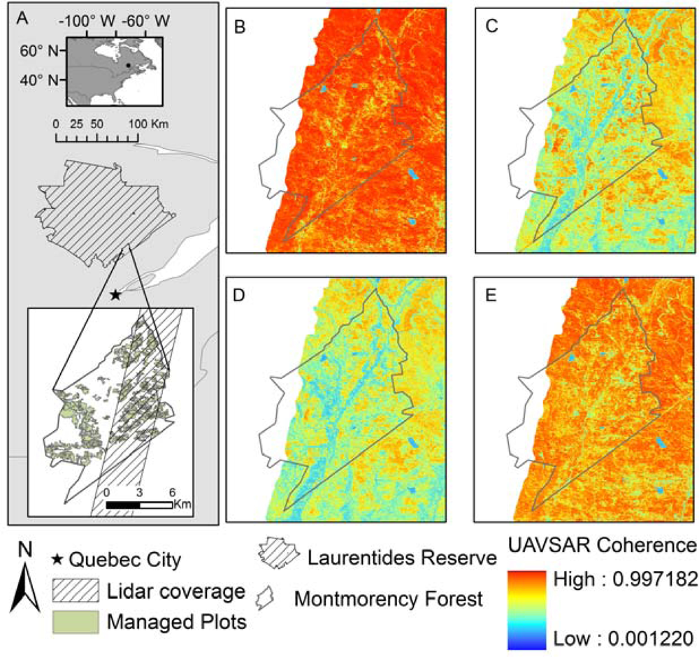
Figure 2.
Weather conditions during UAVSAR acquisition. The rainfall event on 7 August occurred < 3 h before the UAVSAR flight and therefore impacted the coherence estimates for the 2-day interval.
Figure 2.
Weather conditions during UAVSAR acquisition. The rainfall event on 7 August occurred < 3 h before the UAVSAR flight and therefore impacted the coherence estimates for the 2-day interval.
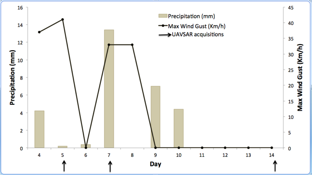
Figure 3.
Variation in stand age in managed patches at Montmorency Forest. Shown here are only patches with >1 ha overlap with the UAVSAR swath.
Figure 3.
Variation in stand age in managed patches at Montmorency Forest. Shown here are only patches with >1 ha overlap with the UAVSAR swath.

Figure 4.
(A) Forest patch age modeled as a function of LVIS waveform metrics. Overlap with LVIS swath is >5 ha. Line fits are added to significant models (see Table 2 for model parameters). (B) Within-patch standard deviation in LVIS-derived canopy height (RH100), showing that mature (>20 years) stands are more homogeneous than young stands.

Figure 5.
Forest patch age modeled as a function of UAVSAR calibrated backscatter. Gridded 5 m resolution γ° values were averaged for each patch. Overlap with UAVSAR swath is >5 ha. Line fits are added to significant models (Table 2).
Figure 5.
Forest patch age modeled as a function of UAVSAR calibrated backscatter. Gridded 5 m resolution γ° values were averaged for each patch. Overlap with UAVSAR swath is >5 ha. Line fits are added to significant models (Table 2).

Figure 6.
Forest patch age modeled as a function of UAVSAR interferometric coherence. Values were calculated with zero spatial baseline and HH polarization. Minimum overlap with UAVSAR swath is 5 ha (top row) and 1 ha (bottom row). Line fits are added to significant models (see Tables 3 and 4 for model parameters). OLS = ordinary least squares, WLS = weighed least squares. Note the broader dynamic range for the 2-day pair.

Figure 7.
Differences in UAVSAR HH coherence between 2-day interval and 7-day temporal baselines. Note there is no temporal overlap between the two pairs (Table 2). The difference shows a marked decrease in coherence for young (<15 years) forest stands. This can explain the reduced model fit for the 7-day pair (Figure 6).

Figure 8.
Actual and modeled patch age from UAVSAR coherence data with zero spatial baseline and 2-day temporal baseline.
Figure 8.
Actual and modeled patch age from UAVSAR coherence data with zero spatial baseline and 2-day temporal baseline.


Table 1.
List of zero baseline UAVSAR coherence pairs. The star (*) represents the polarization channel. Both HH and HV pairs were evaluated.
| Acquisition Day (2009) | UAVSAR Pair | Temporal Baseline |
|---|---|---|
| 7 August | Laurnt_18801_09056_007_090807_L090*_CX_01.grd | 45 min |
| 7 August | Laurnt_18801_09056_005_090807_L090*_CX_01.grd | |
| 14 August | Laurnt_18801_09061_007_090814_L090*_CX_01.grd | 45 min |
| 14 August | Laurnt_18801_09061_005_090814_L090*_CX_01.grd | |
| 5 August | Laurnt_18801_09054_007_090805_L090*_CX_01.grd | 2 days |
| 7 August | Laurnt_18801_09056_007_090807_L090*_CX_01.grd | |
| 7 August | Laurnt_18801_09056_005_090807_L090*_CX_01.grd | 7 days |
| 14 August | Laurnt_18801_09061_007_090814_L090*_CX_01.grd | |
| 5 August | Laurnt_18801_09054_007_090805_L090*_CX_01.grd | 9 days |
| 14 August | Laurnt_18801_09061_007_090814_L090*_CX_01.grd |
Coherence images can be downloaded from the Laurentides Super Site ( http://lidarradar.jpl.nasa.gov/sites/laurentides.html).
Table 2.
Modeling forest patch age from active remote sensing data. Regression equations are of the form Age (years) = a + b × X where X is the predictor variable. Statistically significant models are shown in bold. OLS = ordinary least squares; WLS = weighed least squares. Minimum overlap with UAVSAR/LVIS swath is 5 ha.
| Predictor Variable | R2 | RMSE (years) | a | b | P |
|---|---|---|---|---|---|
| LVIS RH50 | 0.40 | 8.5 | 9.1 | 5.8 | <0.01 |
| LVIS RH75 | 0.29 | 9.2 | 0.8 | 3.9 | <0.01 |
| LVIS RH100 | 0.05 | 10.7 | 4.1 | 1.3 | 0.04 |
| LVIS RH50/RH100 | 0.51 | 7.6 | 5.1 | 100.4 | <0.01 |
| UAVSAR Gamma naught HH | 0.20 | 9.5 | 44.1 | 4.1 | <0.01 |
| UAVSAR Gamma naught HV | 0.37 | 8.4 | 85.7 | 5.1 | <0.01 |
| UAVSAR Gamma naught VV | 0.06 | 10.3 | 41.5 | 2.9 | 0.02 |
| UAVSAR coh HH 45 min | 0.03 | 10.4 | 126.3 | −115.5 | 0.058 |
| UAVSAR coh HH 2 days OLS | 0.75 | 5.3 | 95.3 | −109.2 | <0.01 |
| UAVSAR coh HH 2 days WLS | 0.79 | 19.8 | 93.7 | −104.4 | <0.01 |
| UAVSAR coh HH 7 days OLS | 0.34 | 8.6 | 78.7 | −97.1 | <0.01 |
| UAVSAR coh HH 7 days WLS | 0.59 | 27.9 | 94.0 | −115.1 | <0.01 |
| UAVSAR coh HH 9 days | <0.01 | 10.6 | −4.1 | 25.2 | 0.33 |
Table 3.
Modeling forest patch age from active remote sensing data. Regression equations are of the form Age (years) = a + b × X where X is the predictor variable. Statistically significant models are shown in bold. OLS = ordinary least squares; WLS = weighed least squares. Minimum overlap with UAVSAR/LVIS swath is 1 ha.
| Predictor Variable | R2 | RMSE (years) | a | b | P |
|---|---|---|---|---|---|
| LVIS RH50 | 0.07 | 10.2 | 13.4 | 2.2 | <0.01 |
| LVIS RH75 | 0.01 | 10.6 | 14.0 | 0.7 | 0.10 |
| LVIS RH100 | <0.01 | 10.6 | 20.1 | −0.2 | 0.46 |
| LVIS RH50/RH100 | 0.20 | 9.0 | 44.4 | 4.3 | <0.01 |
| UAVSAR Gamma naught HH | 0.20 | 9.1 | 42.6 | 4.0 | <0.01 |
| UAVSAR Gamma naught HV | 0.30 | 8.5 | 72.5 | 4.2 | <0.01 |
| UAVSAR Gamma naught VV | 0.10 | 9.7 | 42.0 | 3.1 | <0.01 |
| UAVSAR coh HH 45 min | 0.01 | 10.1 | 69.0 | −55.8 | 0.05 |
| UAVSAR coh HH 2 days OLS | 0.67 | 5.8 | 85.7 | −98.1 | <0.01 |
| UAVSAR coh HH 2 days WLS | 0.72 | 23.1 | 91.0 | −103.0 | <0.01 |
| UAVSAR coh HH 7 days OLS | 0.32 | 8.3 | 71.5 | −87.8 | <0.01 |
| UAVSAR coh HH 7 days WLS | 0.52 | 30.4 | 89.1 | −110.0 | <0.01 |
| UAVSAR coh HH 9 days | 0.01 | 10.1 | −4.3 | −25.0 | 0.07 |
Share and Cite
MDPI and ACS Style
Pinto, N.; Simard, M.; Dubayah, R. Using InSAR Coherence to Map Stand Age in a Boreal Forest. Remote Sens. 2013, 5, 42-56. https://doi.org/10.3390/rs5010042
AMA Style
Pinto N, Simard M, Dubayah R. Using InSAR Coherence to Map Stand Age in a Boreal Forest. Remote Sensing. 2013; 5(1):42-56. https://doi.org/10.3390/rs5010042
Chicago/Turabian StylePinto, Naiara, Marc Simard, and Ralph Dubayah. 2013. "Using InSAR Coherence to Map Stand Age in a Boreal Forest" Remote Sensing 5, no. 1: 42-56. https://doi.org/10.3390/rs5010042