Field Imaging Spectroscopy of Beech Seedlings under Dryness Stress
by
 , ,
, ,
Henning Buddenbaum
1,* ,
,
Oksana Stern
1, 
Marion Stellmes
1 ,
,
Johannes Stoffels
1,
Pyare Pueschel
1,
Joachim Hill
1 and
Willy Werner
2 1
Environmental Remote Sensing & Geoinformatics Department, University of Trier, Behringstraße, 54286 Trier, Germany
2
Geobotany Department, University of Trier, Behringstraße, 54286 Trier, Germany
*
Author to whom correspondence should be addressed.
Remote Sens. 2012, 4(12), 3721-3740; https://doi.org/10.3390/rs4123721
Submission received: 3 October 2012
/
Revised: 20 November 2012
/
Accepted: 20 November 2012
/
Published: 26 November 2012
Abstract
:In order to monitor dryness stress under controlled conditions, we set up an experiment with beech seedlings in plant pots and built a platform for observing the seedlings with field imaging spectroscopy. This serves as a preparation for multi-temporal hyperspectral air- and space-borne data expected to be available in coming years. Half of the trees were watered throughout the year; the other half were cut off from water supply for a five-week period in late summer. Plant health and soil, as well as leaf water status, were monitored. Moreover, hyperspectral images of the trees were acquired four times during the experiment. Results show that the experimental imaging setup is well suited for recording hyperspectral images of objects, like the beech pots, under natural illumination conditions. The high spatial resolution makes it feasible to discern between background, soil, wood, green leaves and brown leaves. Furthermore, it could be shown that dryness stress is detectable from an early stage even in the limited spectral range considered. The decline of leaf chlorophyll over time was also well monitored using imaging spectroscopy data.
1. Introduction
One of the major issues in satellite imaging spectroscopy (also known as hyperspectral remote sensing) of vegetation is the timely detection and continuous monitoring of vegetation stress factors. Hyperspectral satellites, like the upcoming EnMAP (Environmental Mapping and Analysis Program [1,2]), will offer the unique possibility to cover large areas with a high temporal and spectral resolution. Enhanced exploitation of the information potential of environmental satellite missions will be particularly helpful for monitoring impacts of climate change and adaptations to climate variability. It is expected that global and regional climate change will lead to more frequent and severe dryness stress, even in regions that so far have not been heavily affected by dryness [3]. For example, the effect of dryness stress on the temperate European forests could be studied in 2003 following an exceptionally dry weather period during summer [4,5].
Reference measurements for air- or spaceborne imaging spectroscopy studies are usually performed using field or laboratory spectrometers that produce one single spectrum per measurement [6]. Especially in remote-sensing-based forest monitoring, there are large differences between reflectance measurements of leaves and reflectance measurements of canopies [7–10]. While it is relatively straightforward to derive plant health indicators like water or chlorophyll content from leaves [11], deriving leaf chemical properties from remotely sensed canopy spectra is still challenging, mainly because of the heterogeneous structure of the crown layer that leads to several levels of clumping and mutual shading [12,13]. Leaf reflectance measurements can be up-scaled to canopy level using a canopy reflectance model. But reflectance measurements on leaf and canopy scale are usually done with completely different sensors. There is clearly a gap between point measurements and the imaging spectroscopy from airborne sensors [14]. Field imaging spectroscopy is a technique that works on a scale between the point measurements of traditional field spectroscopy and airborne imaging spectroscopy and, therefore, can potentially fill this gap.
Another research issue that is of continuous importance is monitoring dryness stress of forests. In central Europe, the sensitivity of beeches to dryness stress depends to a high degree on site conditions [3,15]. The high variability in site conditions (e.g., local topography, soil conditions, climate) as well as the limited availability of a remote sensing time series in high temporal and spatial resolution makes it challenging to study the effects of dryness stress from existing remote sensing data and, thus, to develop remote-sensing-based approaches for monitoring dryness sensitivity in forest ecosystems. One way to tackle this issue is to subject trees to dryness stress in controlled conditions and observe their reactions with imaging spectroscopy.
In order to address these issues, we set up an experiment with beech seedlings in plant pots. Half of the pots were watered all through the year; the other half were cut off from water supply in late summer. Soil and leaf water content and leaf chlorophyll content were measured regularly. At four points in time, images of the beech pots were recorded using a stationary imaging spectrometer that produced very high resolution hyperspectral images in the VNIR spectral range (400 to 1,000 nm). These images were used to characterize the beeches’ reactions to dryness stress. Although the main water absorption bands are located in the SWIR region (1,000 to 2,500 nm), the VNIR spectrometer is able to detect stress symptoms in the chlorophyll absorption bands and in the weak water absorption features around 970 nm [16,17].
The aims of this study were: (1) testing the suitability of the experimental setup and the method of imaging spectroscopy in the VNIR for detecting dryness stress, (2) analyzing the effects of dryness stress under controlled conditions on the spectra, and (3) mapping and analyzing the spatial distribution of these effects in the young trees.
2. Material and Methods
2.1. Planting
We mixed a soil substratum consisting of sand, peat and meadow soil in equal parts. These components were homogeneously mixed and then sterilized overnight using a Mafac Sterilo soil sterilizer. The soil was put into pots of 40 cm diameter in several layers, each with long-term NPK fertilizer and with wicks for irrigation. Each pot was put on a bucket filled with water, with the bottom of the pot 1.5 cm above the water level. The five wicks dip into the water reservoir for supplying the pots with capillary rising moisture through the wicks.
Three four-year old seedlings (ca. 1 m in height) of European Beech (Fagus sylvatica L.) were planted into each pot before leaf flushing in spring. The trees were numbered and then randomly allocated to pots; subsequently, the pots were randomly allocated to dry group and control group. In total, 66 beeches were planted in 22 pots. Five of the pots were excluded from further analyses because the trees did not grow green leaves. Nine control pots and eight dry-group pots were included in the experiment. Additionally, the number of buds was counted on each tree in order to estimate the expected number of leaves. The young beeches were kept under a semi-transparent roof to shield them from rain and direct sunlight.
2.2. Dryness Stress
After an initial growth phase from March to August, half of the pots were cut off from water supply in mid-August, while the other pots (the control group) were continuously watered. The dry group was kept from water supply for five weeks until most signs of dryness stress were clearly visible and many leaves had become brown or rolled up.
Soil water content was measured daily using a TDR probe from the beginning of the drying experiment. Unfortunately, the TDR probe was available only for a limited period until mid-September. Leaf water content was measured at six points in time on up to 49 leaves from trees randomly selected for the leaf sampling. The fresh leaves were weighed, scanned to measure their area, then dried at 105 °C for 24 h and weighed again. Equivalent water thickness (EWT, g/cm2, [18]) was determined by dividing the difference between fresh and dry leaf mass by leaf area.
2.3. Imaging Spectroscopy
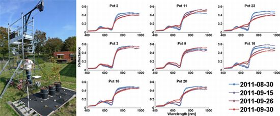
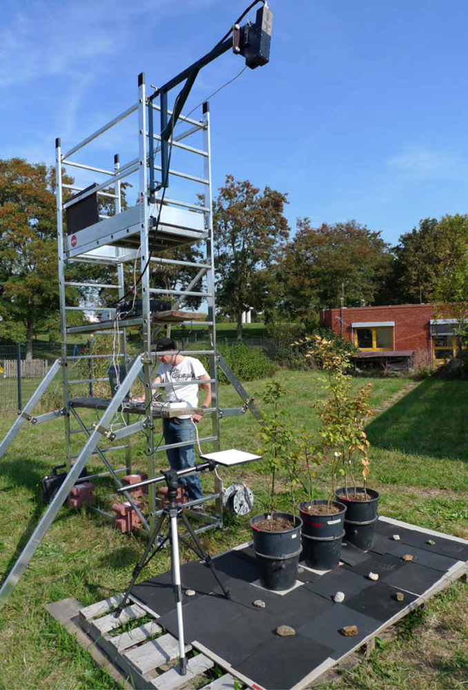
A hyperspectral scanner (NEO HySpex VNIR-1600, [21]) was mounted on a platform about 4 m above ground (Figure 1). The scanner was fixed on a rotation stage that moves the line of sight across the targets acquiring an image composed of scan lines. The instrument has an across-track field of view of 17°, resulting in lines of about 1 m width. The images covered an area of about 3 m × 1 m each. Each image contains two or three pots with near-nadir viewing. The scanner was equipped with a 3 m focal lens with about 0.5 m depth of focus so that most of the area was imaged in focus. A white reference target (Spectralon) of known reflectance was included in the scans in order to convert the recorded radiances to reflectance values. Black foam rubber mats were placed on the ground to reduce stray light from the background. The images were recorded under natural light conditions. Before each scan the integration time was adapted to current brightness. At each of the four imaging days, six images were recorded to cover the 17 pots considered, so a total of 24 hyperspectral images has been utilized in this study.
The camera uses a 2-dimensional CCD sensor array of 320 × 1,600 silicone detectors. One dimension is used for spectral separation and the other dimension is used for imaging in one spatial direction. The second spatial dimension is covered by movement of the sensor. The camera records 1,600 pixels across track, resulting in sub-millimeter spatial resolution. The pixel instantaneous field of view is 0.18 mrad across-track and 0.36 mrad along-track. The speed of the rotation stage was adapted so that an image with approximately square pixels is formed out of the single lines the camera recorded. By binning the 320 sensor pixels in spectral direction, 160 bands were recorded in the spectral range of 410 to 990 nm with a spectral sampling distance of 3.7 nm. Data was recorded in 12 bit radiometric resolution.
Image preprocessing consisted of sensor calibration (converting raw data to radiance and adjusting sensor sensitivity across the line of sight), spatial resampling (merging four pixels into one), division of radiance spectra by mean Spectralon radiance spectrum (conversion from radiance to relative reflectance) and finally spectral resampling for a better signal-to-noise ratio. In the spectral resampling step, the uniform bandwidths were transformed into bandwidths adapted to the signal-to-noise ratio in the respective wavelength region, resulting in 85 bands instead of the original 160 bands. The pixel size depends on distance to the sensor. At 3 m distance, the pixel size after spatial resampling is about 1 mm2.
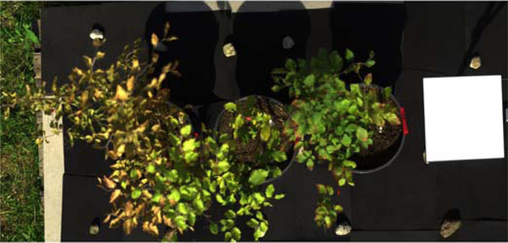
Figure 2 shows a time series of images in true color (RGB = 608 nm, 557 nm, 451 nm). The three pots and the Spectralon white reference can easily be spotted. Each pot contains three trees, but these cannot be discriminated from above. For this reason, spectra have only been extracted for pots, not for single trees. Mean spectra for the respective pots were extracted from the images by manually identifying image regions dominated by leaves. For each region of interest and each time step, the mean spectrum was saved (Figures 3 and 4). These spectra (one spectrum per pot per recording date) were used as training spectra in the following regression analyses.
2.4. Reference Spectroscopic Leaf Measurements
Leaf reflectance in the 350–2,500 nm spectral range was measured at regular intervals using an ASD FieldSpec2 spectroradiometer with a Plant Probe (ASD Inc., Boulder, CO, USA). The Plant Probe consists of a Contact Probe, a spectrometer attachment with a light source covering a 10 mm radius, and a Leaf Clip, a fixture to clamp leaves between the light source/sensor head and an interchangeable black or white background. The Leaf Clip/Contact Probe assembly guarantees constant illumination and viewing geometry and shields the sample from ambient light [22,23].
2.5. Estimation of Equivalent Water Thickness from Imaging Spectroscopy
Spectral indices, like Water Index (WI) [27], Normalized Difference Water Index [28] or Simple Ratio Water Index [29], have been used to estimate vegetation water content from NIR spectroscopy data (refer to [30] for further examples). Among these, only WI, the ratio of reflectance at 900 nm and 970 nm, lies within our sensor’s spectral range. WI was able to explain only 0.36 of the variance of EWT measured.
In order to explore indices of all possible combinations of HySpex bands, we calculated normalized difference indices according to equation (1)
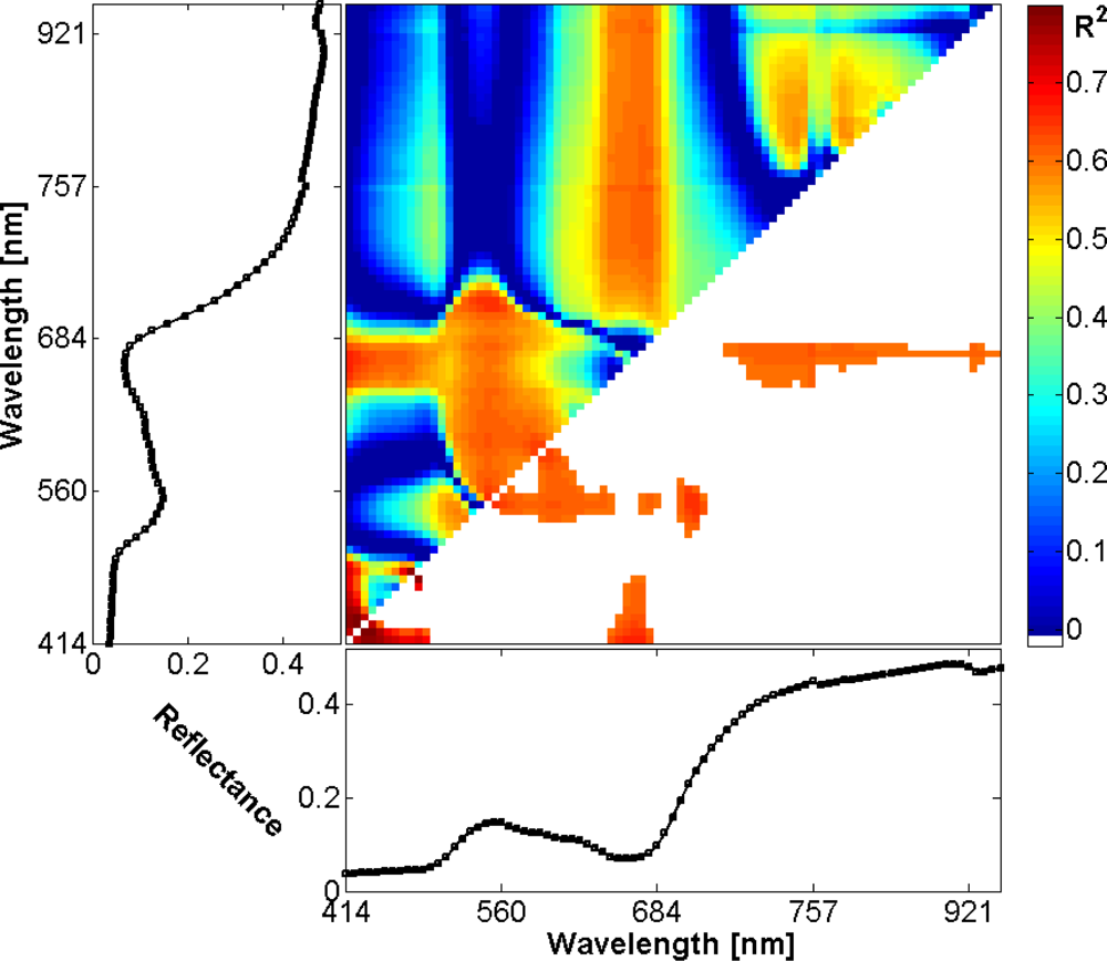
and determined correlation between the index values and measured EWT values. To mitigate overfitting, a leave-on-out cross-validation was applied. As can be seen in the 2D-correlogram in Figure 5 the indices were able to explain up to 0.79 of the EWT variance. The regions that correspond to the highest correlations are highlighted in red and orange in the correlogram [31]: The highest correlations exist between EWT and indices formed solely of bands in the blue spectral region around 450 nm. Further hotspots of correlation are located in the red and green regions (indices similar to PRI [32,33]) and in the region of indices, with one band in the red edge around 700 nm and the other band on the near infrared plateau. For other index types (ratio or difference indices), the results are similar.
Since high R2 estimations of EWT based on two-band indices were spread across the whole spectral range considered, we decided to employ a regression technique that makes use of the full hyperspectral information. Thus, EWT was estimated with a partial least squares regression (PLSR, [34,35]). PLSR is an established robust tool that projects the data into a low-dimensional space formed by a set of orthogonal latent variables by a simultaneous decomposition of X (spectral matrix) and Y (chemical concentration matrix) that maximizes the covariance between X and Y[36]. The method is well suited for calibration on a small number of samples with experimental noise in both chemical and spectral data [37,38]. PLSR is comparable to principal component regression, but differs in that both matrices are simultaneously decomposed.
The PLSR was trained on spectra of the pots and the according gravimetric equivalent water thickness measurements. This leap of scales was intended as a test of PLSR’s ability to estimate a variable of interest from canopy scale spectra, but trained with leaf spectra. One PLSR was used for all time steps. After testing models with 1 to 20 latent variables, we selected a model with five latent variables. Prior to the leaf water estimation, the images were classified using an unsupervised k-mean classifier in order to create a mask of non-leaf pixels. Leaf water content was estimated only for leaf pixels using the PLSR coefficients on image spectra.
2.6. Estimation of Chlorophyll Content from Imaging Spectroscopy
Because chlorophyll is optically active in the spectral region considered with main absorption bands in the blue and red regions, we decided to use a very simple and parsimonious method for chlorophyll content estimation. We calculated a linear regression between a simple vegetation index (Simple Ratio: ρNIR/ρRED, with wavelengths 790 and 670 nm) and Spad chlorophyll measurements for image-based chlorophyll content estimation.
Maps of chlorophyll content were created using this regression to transform Simple Ratio values to Spad values and the empirical polynomial transformation proposed by Markwell et al.[19] for transforming Spad values to chlorophyll concentrations:
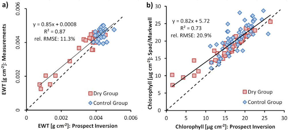
where y is the chlorophyll content in μmol·m−2 and x is the dimensionless Spad meter value. This equation was originally set up for maize and soy bean leaves. In experiments preceding this study (not published), chlorophyll contents of beech and oak leaves were measured with Spad and with acetone extraction in a laboratory, and we found that the equation represents the Spad-chlorophyll relationship for these species as well. Prospect-5b inversions of FieldSpec/PlantProbe leaf reflectance measurements confirmed that the chlorophyll contents derived from Spad measurements are in the correct range of values. In Prospect, chlorophyll content is given as μg·cm−2. By assuming a relative molecular mass for chlorophyll a + b of 900 g·mol−1, the values can be converted from μmol·m−2 to μg·cm−2 by applying a multiplication factor of 0.09.
3. Results and Discussion
3.1. Analysis of the Hyperspectral Images and Spectra
The images recorded are generally of a high signal-to-noise ratio. The spectra are only marginally affected by noise, except for the spectral region beyond 950 nm and in the O2-absorption peak at 760 nm. The black mats, which have a very low reflectance throughout the spectrum, considerably reduced stray light from the background. With the applied settings, one scan takes about two minutes. Some geometric distortions caused by wind-driven leaf movement during the scanning process are clearly visible. We did not apply any geometric correction to the images.
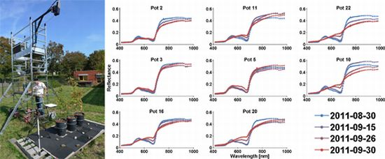
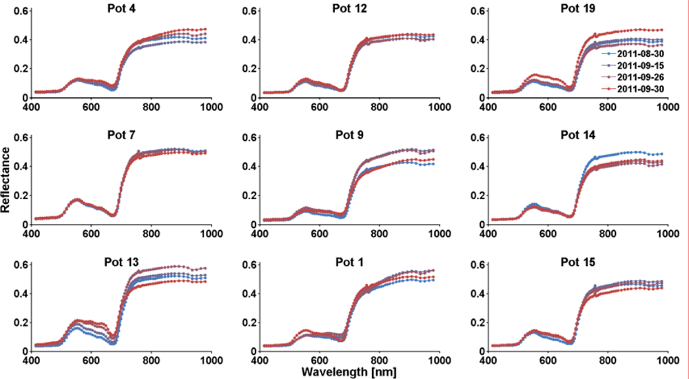
In each image, the areas covered by the beeches of each pot have been manually identified and marked as regions of interest. Mean spectra of these regions were extracted from the images. Figure 3 depicts the temporal change of reflectance of the dry group pots. At the beginning of the experiment the pots were randomly ordered and assigned to control and dry group. Groups of three pots (except for pots 16 and 20) were imaged together at a time; the plots are grouped according to the image recording configurations. Figure 4 shows the according spectra of the control group pots. The spectra show that many of the dry group trees were heavily affected by a browning of leaves in the last two points in time, with first hints of stress already at the second measurement. Most control group spectra do not change much over time. In the control group, only the spectra of pot 13 show clear signs of yellowing, the remaining spectra show the decline of chlorophyll content only subtly in the wavelength region around 600 nm. Changes in general brightness, like those observed in pots 19 and 14, are likely due to the process of extraction the spectra from the image data with different amounts of shadow and differences in leaf orientation in the regions of interest.
3.2. Dryness Stress
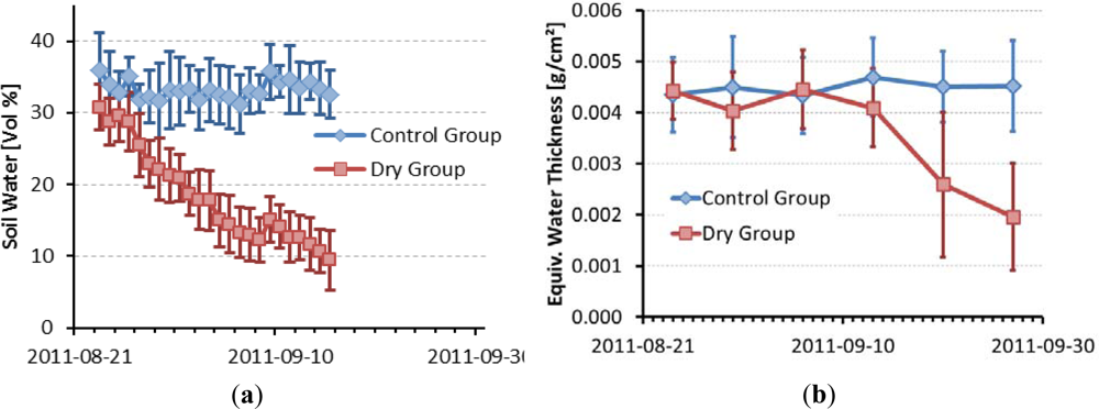
Figure 6(a) shows soil water content measured by TDR probes partitioned for the control group and dry group. The lack of available water for the dry group shows very soon after cutting off water supply. Figure 6(b) and Table 1 show EWT for the two groups. A distinct lag can be witnessed between the quantitative effects of dryness stress on soil and leaf water. EWT stays almost constant during the first four measurements. In the fifth and sixth measurement, EWT of the control group stays constant, while EWT of the dry group decreases. Differences between dry and control group are significant at the fourth measurement and highly significant for the last two measurements. The variance of EWT values is highest in the fifth measurement of the dry group, so is it obvious that not all of the trees suffer from water stress in the same way.
The value range of measured EWT is rather low from the beginning compared to values given in [25] and [39]. In order to confirm these values, EWT was derived from the FieldSpec/PlantProbe reflectance spectra by inverting the Prospect-5b leaf reflectance model. Resulting values correspond well with measured EWT values (Figure 7(a)).
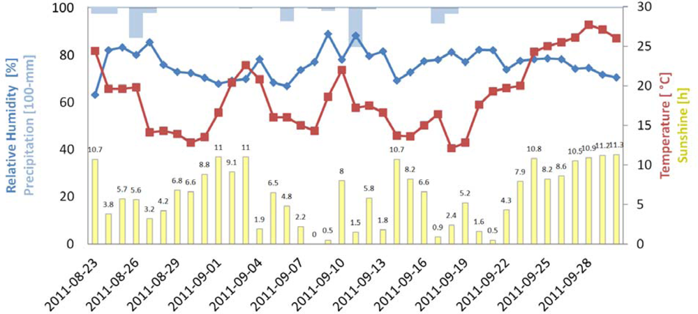
The weather conditions during the experiment are depicted in Figure 8. The trees were kept under a roof, but temperature and humidity were not controlled, so evapotranspiration and the drying rate were affected by the weather. Especially near the end of the experiment, weather conditions were warm and sunny, as reflected in the distinct dryness stress symptoms of the trees.
3.3. Estimation of Equivalent Water Thickness from Imaging Spectroscopy
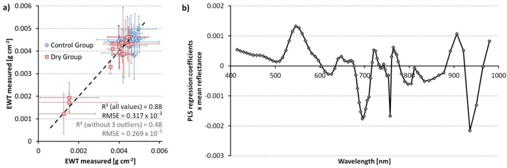
The PLS regression was able to give an unbiased estimation of EWT with a coefficient of determination of R2 = 0.88 (Figure 9(a)). Figure 9(b) shows the PLS regression coefficients of the leaf water content estimation multiplied by the mean reflectance of the training spectra. Leaf water content of a spectrum or a pixel is calculated as the sum of each reflectance value multiplied by its according regression coefficient (inner product) plus an offset. The plot shows the importance of the different wavelength regions for EWT estimation. We see that green wavelengths (around 550 nm) and the red edge region (700 nm) have the largest influence on water content estimation [40]. The NIR plateau region is less important, while the water absorption bands around 970 nm have a high significance [16]. The single negative spike at 757 nm corresponds to the atmospheric oxygen absorption feature. Corresponding spikes can be seen in the reflectance spectra of Figures 3 and 4. We repeated the PLS regression without this wavelength, but no significant difference in the results was detected. The PLS estimation of EWT is quite strongly influenced by the three driest measurements (Figure 9(a)). An alternative PLS model that was trained without these three values reached a coefficient of determination of R2 = 0.48, with very similar PLS regression coefficients. We concluded from this that the model used is stable and not solely dependent on the extreme values and, thus, applied the original model to the image data.
Figure 10 shows maps of EWT as estimated by PLS regression for three pots (pots 10, 5 and 3) over time. The general trend towards dryer leaves is clearly noticeable. Some leaves are dry, even in the first images, and some leaves still have high EWT values in the last images. In Figure 2, one can see that not all the trees are equally affected by dryness stress, so these results seem plausible. Areas with negative estimated EWT values and masked background pixels are displayed in black. Some leaves are displayed enlarged to show within-leaf variation. EWT is highest along the leaf veins and lowest in the areas between them. The enlarged leaf in the second subfigure illustrates this. The within-leaf variations of EWT cannot be studied in detail with this kind of imagery, because many leaves are shaded or obscured by others and leaf orientation varies. The trees in the pot shown on the left side of the figures (pot 10) are most affected by dryness stress, the trees in the pot at the right side (pot 3) are least affected. This corresponds well with the spectra in Figure 3. This variation in sensitivity might be explained by the number of leaves and, as a consequence thereof, increased evapotranspiration rates.
Figure 11 illustrates the relationship between buds counted in spring and EWT at the end of the experiment. This supports the assumption that trees with more leaves were more seriously affected by stress symptoms than trees with fewer leaves.
3.4. Chlorophyll Content
Chlorophyll content declined steadily over time in both the dry group and the control group, as can be seen in Figure 12(a) and in Table 2. Following the drop in EWT, the chlorophyll content of the dry group shows an accelerated decline towards the end of the experiment. While significant differences (p < 0.001) in leaf water content between dry group and control group arise between the 4th and the 5th measurement (between 13 September and 20 September), the chlorophyll contents diverge later, between the 5th and the 6th measurement (between 20 September and 27 September, p < 0.001). The last Spad measurements were only applied on the dry group, after the trees were given water again after the dryness stress experiment. There was a good agreement between the simple ratio calculated from image spectra and the Spad chlorophyll measurements (Figure 12(b)).
There is considerable scatter in Simple Ratio and Spad values of the pots (Figure 12(b)), but, still, the resulting chlorophyll maps are free of image noise and have a reasonable value range and spatial distribution of values. The value range of 100 to 500 μmol·m−2 total chlorophyll corresponds to 9 to 45 μg·cm−2.
Figure 13 shows maps of chlorophyll content for one time series of images created from Simple Ratio calculations as described in Section 2.5. Some leaves in Figure 13 are shown enlarged to illustrate the within-leaf variations of chlorophyll content and the sensor’s ability to map them. Because of the vertical extent of the trees, not all of the leaves are in focus, so that the intra-leaf variability is not apparent for all leaves. Some of the leaves seem to have a margin of low chlorophyll content, but we attribute this to edge effects [41]. Chlorophyll variations along and between the leaf veins can be seen in the zoom images. Detailed analysis of within-leaf variation is not feasible with this kind of imagery, because shading and variations in leaf orientation impede comparability; laboratory imaging spectroscopy of single flattened leaves would be a way to study small-scale variations in chlorophyll content.
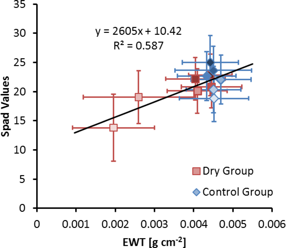
Chlorophyll content and EWT are correlated in our measurements. Figure 14 shows the correlation of all Chlorophyll content and EWT measurements derived from Prospect-5b inversion of FieldSpec reflectance measurements. The correlation coefficient of 0.72 is highly significant (p < 0.001). Since both chlorophyll and mean EWT decline over time, this correlation might be coincidental. Table 3 shows correlation coefficients and significance levels for each measurement time and for all pots, dry group and control group separately, and demonstrates mostly significant correlations during the whole experiment. The correlation analysis does not reveal whether there is a causal relation between the two variables. Since chlorophyll contents of dry group and control group do not differ significantly until after EWT differences have become significant, we assume that the water shortage causes early senescence and thus chlorophyll decomposition in the dry group.
4. Conclusions
This paper describes an experiment where beech seedling were exposed to dryness stress and observed by multi-temporal field imaging spectroscopy. Field imaging spectroscopy in the 400 to 1000 nm wavelength region (VNIR) proved to be a useful tool for estimating dryness stress in beech seedlings on a spatial scale between traditional point reference measurements and airborne remote sensing. We were able to produce millimeter-resolution maps of chlorophyll and water content for the time series. Although the main water absorption bands are located in the SWIR region, the spectra and images recorded still show the process of drying and the resulting stress symptoms quite clearly. The most obvious effect is the browning of leaves, expressed primarily in lower absorption in the red region (600–700 nm) and lower reflectance in the near infrared (700–800 nm, Figures 3 and 4). Figure 9(b) shows the relative importance of the spectral bands for PLSR-based Equivalent Water Thickness (EWT) estimation and demonstrates that the green region (500–600 nm), the red edge region (700 nm) and the water absorption band around 970 nm also have a high importance in vegetation stress monitoring. The experiment started in late summer, when EWT was already quite low, but still the water stress symptoms are detectable and locatable before the leaves become visibly brown.
Both statistical regression methods tested, a simple ratio based linear regression for chlorophyll estimation and a PLS regression for EWT estimation, led to conclusive results. We were able to derive detailed maps of water and chlorophyll content using the hyperspectral images. With these maps, the temporal development of stress symptoms and the differences between the trees, but also variations within the trees, and even variations within single leaves, become visible. Reference measurements of EWT and chlorophyll content (Spad measurements) were made on the leaf scale, but due to the high spatial resolution of the imaging spectrometer, maps at finer scales can be produced. This may lead to some extrapolation problems: The maps include some values that are more extreme than the original measurements. Since the resulting values are still in the same order of magnitude as the training data, we do not consider the extrapolation a major problem.
Although the SWIR domain is expected to have even more potential for dryness stress monitoring, the limited spectral range of our sensor still led to valuable results. Since many lower cost spectrometers, imaging and non-imaging, only work in the 400 to 1,000 nm spectral range, these results are relevant, as they show that even with sub-optimal instrumentation, meaningful results for dryness stress monitoring can be achieved. Further experiments using combined VNIR and SWIR imaging spectroscopy are expected to further enhance the results achieved. Field imaging spectroscopy proved to be a valuable tool for filling the gap between point-based field spectroscopy and airborne imaging spectroscopy.
With the spread of airborne hyperspectral sensors and the expected launch of satellite imaging spectrometers, timely detection of stress in forests seems feasible. Field imaging spectroscopy can complement airborne sensors for algorithm development, since it enables multi-temporal hyperspectral coverage of small targets at much smaller complexity and expenses.
Acknowledgments
We thank our colleagues who assisted in the labor at the greenhouse: Martin Neussel, Thomas Sachtleber, Thomas Lanners and Michael Jeschke who helped in fighting the lice. This research was supported within the framework of the EnMAP project (contract No. 50EE0946-50) by the German Aerospace Center (DLR) and the Federal Ministry of Economics and Technology.
References
- Kaufmann, H.; Segl, K.; Chabrillat, S.; Müller, A.; Richter, R.; Schreier, G.; Hofer, S.; Stuffler, T.; Haydn, R.; Bach, H.; et al. EnMAP—An Advanced Hyperspectral Mission. Proceedings of 4th EARSeL Workshop on Imaging Spectroscopy, Warsaw, Poland, 27–29 April 2005; pp. 55–60.
- Segl, K.; Guanter, L.; Kaufmann, H.; Schubert, J.; Kaiser, S.; Sang, B.; Hofer, S. Simulation of spatial sensor characteristics in the context of the EnMAP hyperspectral mission. IEEE Trans. Geosci. Remote Sens 2010, 48, 3046–3054. [Google Scholar]
- Lindner, M.; Maroschek, M.; Netherer, S.; Kremer, A.; Barbati, A.; Garcia-Gonzalo, J.; Seidl, R.; Delzon, S.; Corona, P.; Kolström, M.; et al. Climate change impacts, adaptive capacity, and vulnerability of European forest ecosystems. For. Ecol. Manage 2010, 259, 698–709. [Google Scholar]
- Bréda, N.; Huc, R.; Granier, A.; Dreyer, E. Temperate forest trees and stands under severe drought: A review of ecophysiological responses, adaptation processes and long-term consequences. Ann. For. Sci 2006, 63, 625–644. [Google Scholar]
- Gobron, N.; Pinty, B.; Mélin, F.; Taberner, M.; Verstraete, M.M.; Belward, A.; Lavergne, T.; Widlowski, J.L. The state of vegetation in Europe following the 2003 drought. Int. J. Remote Sens 2005, 26, 2013–2020. [Google Scholar]
- Milton, E.J.; Schaepman, M.E.; Anderson, K.; Kneubühler, M.; Fox, N. Progress in field spectroscopy. Remote Sens. Environ 2009, 113, S92–S109. [Google Scholar]
- Blackburn, G.A. Quantifying chlorophylls and caroteniods at leaf and canopy scales: An evaluation of some hyperspectral approaches. Remote Sens. Environ 1998, 66, 273–285. [Google Scholar]
- Yoder, B.J.; Pettigrew-Crosby, R.E. Predicting nitrogen and chlorophyll content and concentrations from reflectance spectra (400–2500 nm) at leaf and canopy scales. Remote Sens. Environ 1995, 53, 199–211. [Google Scholar]
- Verhoef, W.; Bach, H. Coupled soil-leaf-canopy and atmosphere radiative transfer modeling to simulate hyperspectral multi-angular surface reflectance and TOA radiance data. Remote Sens. Environ 2007, 109, 166–182. [Google Scholar]
- Asner, G.P.; Martin, R.E.; Knapp, D.E.; Tupayachi, R.; Anderson, C.; Carranza, L.; Martinez, P.; Houcheime, M.; Sinca, F.; Weiss, P. Spectroscopy of canopy chemicals in humid tropical forests. Remote Sens. Environ 2011, 115, 3587–3598. [Google Scholar]
- Curran, P.J. Remote sensing of foliar chemistry. Remote Sens. Environ 1989, 30, 271–278. [Google Scholar]
- Buddenbaum, H.; Pueschel, P.; Stellmes, M.; Werner, W.; Hill, J. Measuring water and Chlorophyll content on the leaf and canopy scale. EARSeL eProc 2011, 10, 66–72. [Google Scholar]
- Schlerf, M.; Atzberger, C.; Hill, J.; Buddenbaum, H.; Werner, W.; Schüler, G. Retrieval of chlorophyll and nitrogen in Norway spruce (Picea abies L. Karst.) using imaging spectroscopy. Int. J. Appl. Earth Obs. Geoinf 2010, 12, 17–26. [Google Scholar]
- d’Oleire-Oltmanns, S.; Marzolff, I.; Peter, K.; Ries, J. Unmanned Aerial Vehicle (UAV) for monitoring soil erosion in Morocco. Remote Sens 2012, 4, 3390–3416. [Google Scholar]
- Hill, J.; Stellmes, M.; Stoffels, J.; Werner, W.; Shtern, O.; Frantz, D. Assessing the Sensitivity of European Beech (Fagus sylvatica L.) Stands to Severe Drought Based on Measurements from Earth Observation Satellites. Proceedings of 1st Forestry Workshop: Operational Remote Sensing in Forest Management, Prague, Czech Republic, 2–3 June 2011.
- Sims, D.A.; Gamon, J.A. Estimation of vegetation water content and photosynthetic tissue area from spectral reflectance: A comparison of indices based on liquid water and chlorophyll absorption features. Remote Sens. Environ 2003, 84, 526–537. [Google Scholar]
- Peñuelas, J.; Piñol, J.; Ogaya, R.; Filella, I. Estimation of plant water concentration by the reflectance Water Index WI (R900/R970). Int. J. Remote Sens 1997, 18, 2869–2875. [Google Scholar]
- Datt, B. Remote Sensing of water content in Eucalyptus leaves. Aust. J. Bot 1999, 47, 909–923. [Google Scholar]
- Markwell, J.; Osterman, J.C.; Mitchell, J.L. Calibration of the Minolta SPAD-502 leaf chlorophyll meter. Photosynth. Res 1995, 46, 467–472. [Google Scholar]
- Uddling, J.; Gelang-Alfredsson, J.; Piikki, K.; Pleijel, H. Evaluating the relationship between leaf chlorophyll concentration and SPAD-502 chlorophyll meter readings. Photosynth. Res 2007, 91, 37–46. [Google Scholar]
- Buddenbaum, H.; Steffens, M. Laboratory imaging spectroscopy of soil profiles. J. Spect. Imag 2011, 2, 1–5. [Google Scholar]
- Castro-Esau, K.L.; Sánchez-Azofeifa, G.A.; Rivard, B. Comparison of spectral indices obtained using multiple spectroradiometers. Remote Sens. Environ 2006, 103, 276–288. [Google Scholar]
- Delalieux, S.; Auwerkerken, A.; Verstraeten, W.; Somers, B.; Valcke, R.; Lhermitte, S.; Keulemans, J.; Coppin, P. Hyperspectral reflectance and fluorescence imaging to detect scab induced stress in apple leaves. Remote Sens 2009, 1, 858–874. [Google Scholar]
- Feret, J.-B.; François, C.; Asner, G.P.; Gitelson, A.A.; Martin, R.E.; Bidel, L.P.R.; Ustin, S.L.; le Maire, G.; Jacquemoud, S. PROSPECT-4 and 5: Advances in the leaf optical properties model separating photosynthetic pigments. Remote Sens. Environ. 2008, 112, 3030–3043. [Google Scholar]
- Jacquemoud, S.; Baret, F. PROSPECT: a model of leaf optical properties spectra. Remote Sens. Environ 1990, 34, 75–91. [Google Scholar]
- Jacquemoud, S. Prospect + Sail = Prosail. Available online: http://teledetection.ipgp.jussieu.fr/prosail/ (accessed on 23 November 2012).
- Peñuelas, J.; Filella, I.; Biel, C.; Serrano, L.; Savé, R. The reflectance at the 950–970 nm region as an indicator of plant water status. Int. J. Remote Sens 1993, 14, 1887–1905. [Google Scholar]
- Gao, B.-C. NDWI—A normalized difference water index for remote sensing of vegetation liquid water from space. Remote Sens. Environ 1996, 58, 257–266. [Google Scholar]
- Zarco-Tejada, P.J.; Rueda, C.A.; Ustin, S.L. Water content estimation in vegetation with MODIS reflectance data and model inversion methods. Remote Sens. Environ 2003, 85, 109–124. [Google Scholar]
- Thenkabail, P.S.; Lyon, J.G.; Huete, A. Optical Remote Sensing of Vegetation Water Content. In Hyperspectral Remote Sensing of Vegetation; CRC Press: Boca Raton, FL, USA/London, UK/New York, NY, USA, 2012; pp. 227–244. [Google Scholar]
- Schlerf, M.; Atzberger, C.; Hill, J. Remote sensing of forest biophysical variables using HyMap imaging spectrometer data. Remote Sens. Environ 2005, 95, 177–194. [Google Scholar]
- Gamon, J.A.; Peñuelas, J.; Field, C.B. A narrow-waveband spectral index that tracks diurnal changes in photosynthetic efficiency. Remote Sens. Environ 1992, 41, 35–44. [Google Scholar]
- Gamon, J.A.; Serrano, L.; Surfus, J.S. The photochemical reflectance index: An optical indicator of photosynthetic radiation use efficiency across species, functional types, and nutrient levels. Oecologia 1997, 112, 492–501. [Google Scholar]
- Wold, S.; Sjöström, M.; Eriksson, L. PLS-regression: A basic tool of chemometrics. Chemometr. Intell. Lab. Syst 2001, 58, 109–130. [Google Scholar]
- Wold, S.; Trygg, J.; Berglund, A.; Antti, H. Some recent developments in PLS modeling. Chemometr. Intell. Lab. Syst 2001, 58, 131–150. [Google Scholar]
- Vohland, M.; Emmerling, C. Determination of total soil organic C and hot water-extractable C from VIS-NIR soil reflectance with partial least squares regression and spectral feature selection techniques. Eur. J. Soil Sci. 2011, 598–606. [Google Scholar]
- Atzberger, C.; Guérif, M.; Baret, F.; Werner, W. Comparative analysis of three chemometric techniques for the spectroradiometric assessment of canopy chlorophyll content in winter wheat. Comput. Electron. Agr 2010, 73, 165–173. [Google Scholar]
- Eisele, A.; Lau, I.; Hewson, R.; Carter, D.; Wheaton, B.; Ong, C.; Cudahy, T.J.; Chabrillat, S.; Kaufmann, H. Applicability of the thermal infrared spectral region for the Prediction of soil properties across semi-arid agricultural landscapes. Remote Sens 2012, 4, 3265–3286. [Google Scholar]
- Féret, J.-B.; François, C.; Gitelson, A.; Asner, G.P.; Barry, K.M.; Panigada, C.; Richardson, A.D.; Jacquemoud, S. Optimizing spectral indices and chemometric analysis of leaf chemical properties using radiative transfer modeling. Remote Sens. Environ 2011, 115, 2742–2750. [Google Scholar]
- Nansen, C. Use of variogram parameters in analysis of hyperspectral imaging data acquired from dual-stressed crop leaves. Remote Sens 2012, 4, 180–193. [Google Scholar]
- Eitel, J.U.H.; Vierling, L.A.; Long, D.S. Simultaneous measurements of plant structure and chlorophyll content in broadleaf saplings with a terrestrial laser scanner. Remote Sens. Environ 2010, 114, 2229–2237. [Google Scholar]
Figure 1.
Setup for field imaging spectroscopy: Three pots with three beech seedlings each and a white reference are recorded.
Figure 1.
Setup for field imaging spectroscopy: Three pots with three beech seedlings each and a white reference are recorded.

Figure 2.
True color depictions of HySpex images of pots 10, 5, and 3. The images were recorded (top to bottom) 2011-08-30, 2011-09-15, 2011-09-26, and 2011-09-30. White reference panel can be seen in the right part of each image.
Figure 2.
True color depictions of HySpex images of pots 10, 5, and 3. The images were recorded (top to bottom) 2011-08-30, 2011-09-15, 2011-09-26, and 2011-09-30. White reference panel can be seen in the right part of each image.
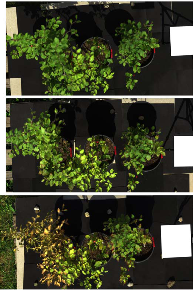

Figure 3.
HySpex reflectance spectra of dry group pots (mean spectra of 37,000 to 167,000 pixels).
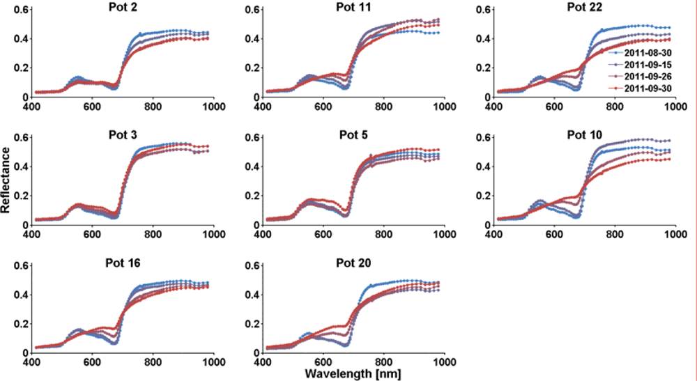
Figure 4.
HySpex reflectance spectra of control group pots (mean spectra of 38,000 to 225,000 pixels).
Figure 4.
HySpex reflectance spectra of control group pots (mean spectra of 38,000 to 225,000 pixels).

Figure 5.
Map of R2 values of normalized difference indices of all possible band combinations and EWT. In the lower part of the correlogram, only values of R2 > 0.6 are shown. The graphs below and left of the correlogram contain the mean reflectance of the training areas.
Figure 5.
Map of R2 values of normalized difference indices of all possible band combinations and EWT. In the lower part of the correlogram, only values of R2 > 0.6 are shown. The graphs below and left of the correlogram contain the mean reflectance of the training areas.

Figure 6.
(a) Temporal development of soil water content in dry group and control group. The error bars indicate ±1 standard deviation between the pots of the groups. (b) Leaf water content of dry group and control group. Error bars indicate ±1 standard deviation of the leaves in each group.
Figure 6.
(a) Temporal development of soil water content in dry group and control group. The error bars indicate ±1 standard deviation between the pots of the groups. (b) Leaf water content of dry group and control group. Error bars indicate ±1 standard deviation of the leaves in each group.

Figure 7.
(a) EWT from Prospect inversion and measured EWT; (b) chlorophyll content from Prospect inversion and chlorophyll content measured with Spad, converted into μmol·m−2 by Markwell equation and into μg·cm−2 by multiplication with 0.09, both with 1:1 line (dashed) and regression.
Figure 7.
(a) EWT from Prospect inversion and measured EWT; (b) chlorophyll content from Prospect inversion and chlorophyll content measured with Spad, converted into μmol·m−2 by Markwell equation and into μg·cm−2 by multiplication with 0.09, both with 1:1 line (dashed) and regression.

Figure 8.
Weather conditions for the time of the dryness stress experiment.

Figure 9.
(a) PLS regression of equivalent water thickness derived from tree spectra with 1:1 line; horizontal and vertical error bars indicate standard deviation of measurements and PLSR-estimated water contents within the pots, respectively; (b) PLS regression coefficients multiplied by mean reflectance in the respective wavelength.

Figure 10.
Maps of EWT over time, estimated by PLSR. Some leaves are shown enlarged.

Figure 11.
Relationship between the number of buds counted in spring and EWT at the end of the experiment for the dry group.
Figure 11.
Relationship between the number of buds counted in spring and EWT at the end of the experiment for the dry group.
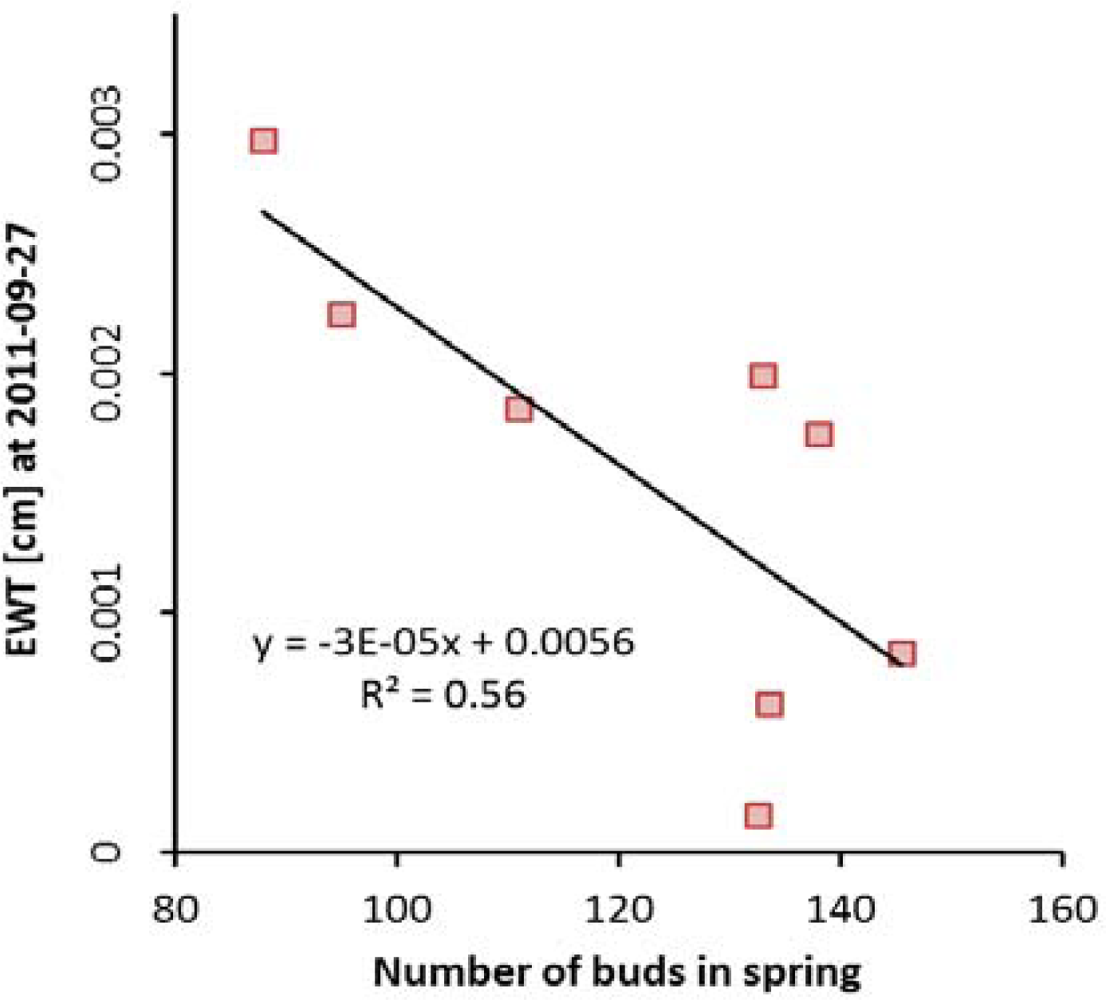
Figure 12.
(a) Chlorophyll content of dry group and control group measured with Spad. Error bars indicate ±1 standard deviation of the leaves in each group. (b) A simple ratio estimation of chlorophyll content. Error bars indicate ±1 standard deviation of Spad and of simple ratio values per pot.
Figure 12.
(a) Chlorophyll content of dry group and control group measured with Spad. Error bars indicate ±1 standard deviation of the leaves in each group. (b) A simple ratio estimation of chlorophyll content. Error bars indicate ±1 standard deviation of Spad and of simple ratio values per pot.
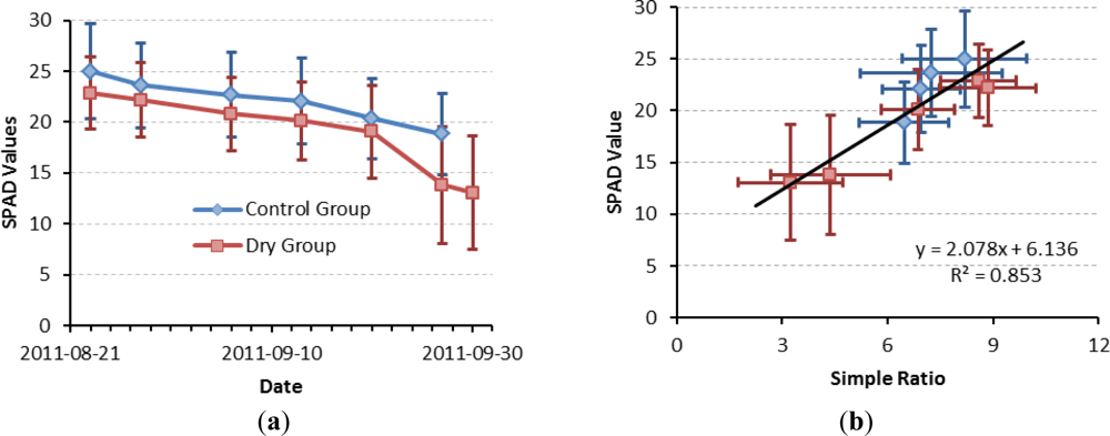
Figure 13.
Maps of chlorophyll concentration, derived via Simple Ratio. Some leaves are shown enlarged.
Figure 13.
Maps of chlorophyll concentration, derived via Simple Ratio. Some leaves are shown enlarged.

Figure 14.
Correlation between Spad values and EWT for all measuring dates combined. Lighter symbols correspond to later measurement date. Error bars indicate ± 1 standard deviation.
Figure 14.
Correlation between Spad values and EWT for all measuring dates combined. Lighter symbols correspond to later measurement date. Error bars indicate ± 1 standard deviation.

Table 1.
Basic statistics of EWT measurements and significance (p) of t-tests of differences between groups (*: p < 0.05, **: p < 0.01, ***: p < 0.001)
| Date | 2011-08-24 | 2011-08-30 | 2011-09-06 | 2011-09-13 | 2011-09-20 | 2011-09-27 |
|---|---|---|---|---|---|---|
| Mean Dry Group | 0.00442 | 0.00404 | 0.00445 | 0.00409 | 0.00259 | 0.00195 |
| StDev Dry Group | 0.00055 | 0.00076 | 0.00077 | 0.00076 | 0.00141 | 0.00104 |
| Mean Control Group | 0.00442 | 0.00450 | 0.00433 | 0.00469 | 0.00450 | 0.00452 |
| StDev Control Group | 0.00072 | 0.00098 | 0.00074 | 0.00076 | 0.00069 | 0.00089 |
| Significance of t-test | 0.4996 | 0.0492* | 0.3090 | 0.0092** | 4.87E-06*** | 2.89E-09*** |
Table 2.
Basic statistics of chlorophyll a + b measurements and significance of t-tests of differences between groups (*: p < 0.05, **: p < 0.01, ***: p < 0.001).
| Date | 2011-08-23 | 2011-08-28 | 2011-09-06 | 2011-09-13 | 2011-09-20 | 2011-09-27 |
|---|---|---|---|---|---|---|
| Mean Dry Group | 22.86 | 22.18 | 20.81 | 20.12 | 19.04 | 13.80 |
| StDev Dry Group | 3.56 | 3.66 | 3.61 | 3.83 | 4.53 | 5.73 |
| Mean Control Group | 25.00 | 23.62 | 22.68 | 22.07 | 20.35 | 18.84 |
| StDev Control Group | 4.63 | 4.18 | 4.18 | 4.22 | 3.95 | 3.97 |
| Significance of t-test | 0.050* | 0.125 | 0.063 | 0.059 | 0.156 | 0.0007*** |
Table 3.
Correlation between chlorophyll content and EWT (derived from Prospect-5b inversion of FieldSpec leaf reflectance measurements) for all measuring dates (°: p < 0.1, *: p < 0.05, **: p < 0.01, ***: p < 0.001).
| Measuring Dates | 08-23/24 | 08-30/31 | 09-06/07 | 09-13/14 | 09-20/21 | 09-27/28 |
|---|---|---|---|---|---|---|
| Correlation all pots | 0.45** | 0.46** | 0.37* | 0.56*** | 0.63*** | 0.77*** |
| Correlation dry group | 0.30 | 0.34 | 0.38° | 0.55** | 0.56** | 0.77*** |
| Correlation control group | 0.63** | 0.63** | 0.37° | 0.56** | 0.56** | 0.53* |
Share and Cite
MDPI and ACS Style
Buddenbaum, H.; Stern, O.; Stellmes, M.; Stoffels, J.; Pueschel, P.; Hill, J.; Werner, W. Field Imaging Spectroscopy of Beech Seedlings under Dryness Stress. Remote Sens. 2012, 4, 3721-3740. https://doi.org/10.3390/rs4123721
AMA Style
Buddenbaum H, Stern O, Stellmes M, Stoffels J, Pueschel P, Hill J, Werner W. Field Imaging Spectroscopy of Beech Seedlings under Dryness Stress. Remote Sensing. 2012; 4(12):3721-3740. https://doi.org/10.3390/rs4123721
Chicago/Turabian StyleBuddenbaum, Henning, Oksana Stern, Marion Stellmes, Johannes Stoffels, Pyare Pueschel, Joachim Hill, and Willy Werner. 2012. "Field Imaging Spectroscopy of Beech Seedlings under Dryness Stress" Remote Sensing 4, no. 12: 3721-3740. https://doi.org/10.3390/rs4123721