Characterization of Rape Field Microwave Emission and Implications to Surface Soil Moisture Retrievals


1
Department of Geography, University of Munich, Luisenstr. 37, D-80333 Munich, Germany
2
Institute of Meteorology and Climate Research, Karlsruhe Institute of Technology, D-82467 Garmisch-Partenkirchen, Germany
3
Max-Planck-Institute for Meteorology, KlimaCampus, D-20146 Hamburg, Germany
*
Author to whom correspondence should be addressed.
Remote Sens. 2012, 4(1), 247-270; https://doi.org/10.3390/rs4010247
Submission received: 4 November 2011
/
Revised: 4 January 2012
/
Accepted: 4 January 2012
/
Published: 16 January 2012
Abstract
:In the course of Soil Moisture and Ocean Salinity (SMOS) mission calibration and validation activities, a ground based L-band radiometer ELBARA II was situated at the test site Puch in Southern Germany in the Upper Danube Catchment. The experiment is described and the different data sets acquired are presented. The L-band microwave emission of the biosphere (L-MEB) model that is also used in the SMOS L2 soil moisture algorithm is used to simulate the microwave emission of a winter oilseed rape field in Puch that was also observed by the radiometer. As there is a lack of a rape parameterization for L-MEB the SMOS default parameters for crops are used in a first step which does not lead to satisfying modeling results. Therefore, a new parameterization for L-MEB is developed that allows us to model the microwave emission of a winter oilseed rape field at the test site with better results. The soil moisture retrieval performance of the new parameterization is assessed in different retrieval configurations and the results are discussed. To allow satisfying results, the periods before and after winter have to be modeled with different parameter sets as the vegetation behavior is very different during these two development stages. With the new parameterization it is possible to retrieve soil moisture from multiangular brightness temperature data with a root mean squared error around 0.045–0.051 m3/m3 in a two parameter retrieval with soil moisture and roughness parameter Hr as free parameters.
1. Introduction
Controlling the energy- and mass exchanges between the Earth’s surface and the atmosphere, the water content of the upper soil layer plays an important role within the global, regional and local water cycle and thus, the global climate system. Evaporation rates, surface runoff, infiltration as well as plant growth and photosynthetic activity are controlled by the water content of the soil [1,2]. Observations of soil moisture serve as input for numerical weather and climate prediction models and are needed for hydrologic modeling, flood and drought monitoring and other water and energy cycle applications [2,3].
Several remote sensing techniques have been tested for measuring variations of soil moisture on different scales [4–7]. Amongst these, passive microwave systems have proven to be very promising as this technique benefits from being almost independent from solar radiation and weather conditions. Microwave emissions show a direct relationship to soil moisture through the soil’s dielectric constant and have a sensitivity to land surface roughness and vegetation cover [8].
At L-Band (21 cm, 1.4 GHz), soil moisture in the first centimeters of the soil has a significant impact on the emitted brightness temperature TB (about 2 K per 0.01 [m3/m3] over bare soil [2]). The SMOS (Soil Moisture and Ocean Salinity) mission (launched in 2009) was designed to measure soil moisture and ocean salinity from space with a repetition rate of 1–3 days and a spatial resolution of 35–50 km with the unique MIRAS (microwave imaging radiometer with aperture synthesis) 2D interferometric L-band radiometer (1.4 GHz) [2]. Through the exceptional measurement technique it is possible to separate vegetation- and soil moisture dynamics through multiangular (0° to 55°) brightness temperature measurements [2].
To investigate passive microwave remote sensing of soil moisture under different canopy types, a variety of campaigns with ground- or aircraft-based L-Band radiometers were carried out in the past [9]. These experiments are being used to develop, improve and calibrate radiative transfer modeling which is essential for soil moisture retrieval from passive microwave data. In preparation for the SMOS mission, several dedicated ground radiometer experiments were conducted. Examples for these experiments are the long term radiometer field experiment SMOSREX [10] that is carried out over bare and vegetated soil near Toulouse in South France with the (LEWIS) L-Band radiometer and the Bray 2004 experiment in the Les Landes forest near Bordeaux [11]. Further Schwank et al. performed a L-Band radiometer experiment at the test site Eschikon near Zurich, Switzerland for clover grass in 2007 [12] as well as in 2004 over a freezing soil [13] which was successfully used for the parameterization and assimilation into a hydrological model [14,15]. Wigneron et al. [9] gives an overview about the L-Band radiometer experiments that have been used for the development of the radiative transfer model used in the SMOS L2 soil moisture processor. A new generation of L-Band radiometers are the ELBARA II radiometers (ETH L-Band Radiometer 2nd generation) that are used throughout Europe for dedicated studies in the SMOS context [16]. Examples are the experiments in Valencia, Spain [17], Sodankyla, Finland [18], Grenoble, France and Puch near Munich, Germany [19].
It is the scope of this paper to describe the experiment carried out in Puch in Southern Germany as well as describe the microwave emission of winter oilseed rape as measured in Puch and establish a parameterization that allows modeling the brightness temperature with the radiative transfer model L-MEB that is also used in the SMOS L2 soil moisture processor. The soil moisture retrieval capabilities of L-MEB over winter oilseed rape are assessed.
Although many microwave emission experiments with different vegetation types have taken place in the past, there is no study to the author’s knowledge about winter oilseed rape, consequently no parameters are known for representing it in L-MEB. In Germany, rape was one of the three most important crops grown in 2010. With around 155,000 ha, rape plays an important role within the renewable energy sector because it serves as basis for alternative energy- and industrial-production [20]. Therefore it should be of interest how that crop behaves in radiative transfer modeling.
In Section 2, the field experiment is described according to geographical location of the test site and data sets being used in the present study. The following Section 3 elaborates on the model L-MEB and how it is being used. Section 4 presents the results of the microwave emission modeling and the soil moisture retrieval capabilities of the model for the land use winter oilseed rape. A discussion of the results as well as a conclusion is added to complete the paper.
2. Field Experiment
2.1. Test Site
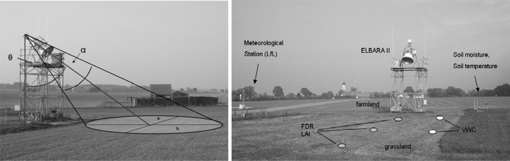
In the course of SMOS cal/val activities, one of the passive microwave radiometers ELBARA II was installed on a well instrumented experimental farm of the Bavarian State Research Center for Agriculture (LfL) in Puch, about 30 km west of Munich in Southern Germany in the center of the SMOS test site Upper Danube [19,21,22] (Figure 1). The intention of the experiment was to measure brightness temperatures (TB) constantly over two vegetative surfaces: grassland and farmland, which was in this case cultivated with winter oilseed rape. Extensive ancillary environmental data have been collected in addition to constant measuring stations.
The location of the radiometer has the geographical coordinates 11.2136°E and 48.1845°N and it is 556 m a.s.l. [19]. It is situated in the temperate latitudes of Central Europe within the region of the northern Alpine foreland. The climate can be described as temperate humid with a maximum of precipitation during summer [23]. The soil type was classified as sandy loam with a sand content of 22% and a clay content of 6% and a bulk soil density of 1.2 g/cm3. The radiometer test site is surrounded by a flat agricultural area. At the border of two fields of different land use (grassland and farmland), the passive microwave radiometer ELBARA II had been installed on a scaffolding of 4 m in such a way that it was possible to rotate the radiometer in order to measure over two types of land use. Due to technical restraints the viewing angles over the two fields could only be varied between 50° and 70°. Schwank et al. [16] give a detailed overview of the technical details of the radiometer. In the surroundings of the radiometer, ground measurements (vegetation height, leaf area index (LAI), phenology, vegetation water content (VWC), soil roughness, soil moisture, snow parameters) were conducted on a regular basis and continuous hourly measurement stations of soil moisture and soil temperature were set up. Data of the meteorological station of the Bavarian State Research Center for Agriculture next to the radiometer were used for completing the data set.
Figure 2 shows the radiometer ELBARA II with angle of aperture α and incidence angle θ and the location of ground truth measurements.
2.2. Measurements
All ground measurements were collected from 1 October 2009 until 14 July 2010. The period of 287 days is approximately the duration of the vegetation period of winter oilseed rape at the location Puch. Days with snow cover or frozen ground were removed from the data sets for the current analysis. In addition to these gaps some technical problems resulted in data loss which extended the data gaps in winter. All measurements related to soil moisture and vegetation characteristics were carried out on a weekly basis if the weather conditions permitted it.
2.2.1. Meteorological and Soil Moisture Measurements
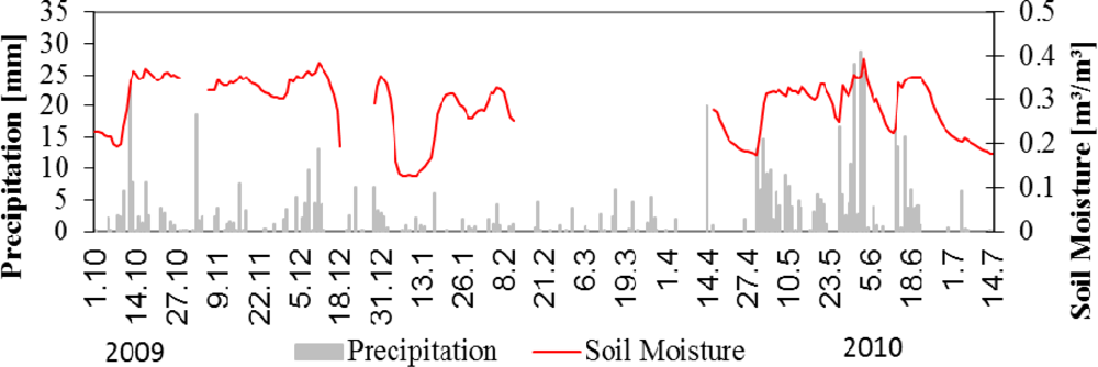
From the start of the experiment in October 2009 to July 2010 the mean temperature measured 2 m above the soil surface was 9.3 °C. The total precipitation during the campaign was 599.5 mm, with a maximum daily rain event on 2 June 2010 of 28.8 mm·d−1.
Soil moisture and soil temperature stations at two locations (farmland and grassland) next to the radiometer tower were installed at the beginning of the campaign to record the development of soil moisture and soil temperature profiles. Soil water content and temperatures were measured hourly with horizontally installed IMKO Trime-TDR (time domain reflectometry) probes in several depths (5, 10, 20 and 40 cm for soil moisture and 2, 5 and 50 cm for soil temperature). For quality control of the station measurements, handheld measurements of soil water content were conducted on a weekly basis at the stations and inside the field of view (FOV) of the radiometer at three sampling points. As the station measurements seem very reliable they are considered representative for the radiometer FOV. Figure 3 shows the development of the measured surface soil moisture and the precipitation throughout the study period.
2.2.2. Vegetation Measurements
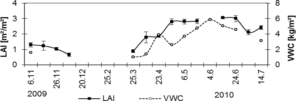
The vegetation on the farmland area that is subject of this study was winter oilseed rape (brassica napus), sowing is dated to 21 August 2009. About 30 days after seeding, the first sprouts became visible. During presence of vegetation, the LAI was measured using a LAICOR LAI-2000 [24], the vegetation water content [kg·m−2] was measured through destructive measurements. The LAI and vegetation height were measured at the sampling points inside and outside the FOV while the vegetation water content was only measured outside the FOV in order to not disturb the radiometer measurements (Figure 3). The development of the LAI as well as the VWC is shown in Figure 4.
The vegetation height ranged from 15 cm in the beginning of November 2009 to 135 cm at the end of the growing period mid of July 2010. The LAI increased from 1.5 to 3 m2/m2 and the water content from 0.5 to approx. 6 kg/m2. The correlation of LAI and VWC gives an R2 of 0.77 and a regression function of VWC = 1.571 × LAI − 0.320.
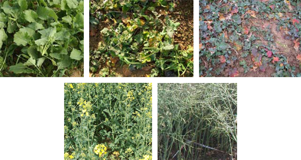
The typical vegetation development of winter rape as described in [25] was confirmed by the measurements of vegetation height, LAI, VWC and observations of phenology. After emergence of the first plants in autumn, the three parameters: height, LAI and VWC increased until the daily mean temperature fell below a value of 5 °C. With this temperature the first plants start to degenerate, until the beginning of winter period, with nearly no ‘vital vegetation’ left (see Figure 5). This effect also shows in rape leaves turning brown during winter. The snow layer during winter protected the plants from frost. During snow cover the maximum snow height reached 17cm at the beginning of February.
With the end of winter, the former horizontally oriented leaves then turned to vertical growth with the formation of branches until the canopy reached its maximum height. With the end of the growing period, the plants lost most of their leaves, only the pods remained. The winter break naturally divides the vegetation growth into two periods with very different appearance of the plants.
The vegetation grew with a rate of about 0.87 cm day−1 from 40 to 140 cm, during the main growing period of 92 days from 25 March until 24 June 2010. The density of dry-matter increased with approximately 44 g·m−2·d−1 during the same time.
2.2.3. Surface Roughness Measurements
A photogrammetric approach was chosen for roughness measurements at the test site due to its 3 dimensional output and highly accurate estimates [26]. For sampling soil surface roughness, a rectangular scaffold with the dimensions of 1 × 2.5 m2 was laid onto the ground and used as a reference frame for the orientation of the image block. As the sample plots were entirely covered by vegetation during the test period, all the plants in the sampling area were cut off and removed without disturbing the soil surface. Highly precise ground control points (GCP) attached to the scaffold made it possible, to generate a digital elevation model (DEM) out of overlapping photos shot from around 2.5 m height by using image matching techniques. More detailed information of the measurement technique is given in [27]. Figure 6 shows an example of one DEM with heights in cm and relative to the lower edge of the scaffold containing a tractor track (this one was not used in the current study as it is not representative for the radiometer FOV). From the DEM it was possible to calculate the RMS-Height s (standard deviation of height) [cm] for the entire area, which gives a direct information on the (vertical) roughness condition [28,29].
As [30] was able to establish a clear relationship between s and Hr but obtained no improvement in the parameterization of Hr by using additional information like the autocorrelation length, s is the only parameter considered in this study.
Roughness measurements were conducted in September 2009, March and September 2010. The results from the roughness measurements are listed in Table 1. The value s describes the standard deviation of surface heights related to the lower edge of the scaffold in cm. At three locations within the field roughness measurements were taken near the radiometer FOV and then averaged.
s varies from 1.0 to 1.3 cm in the course of the measurement period which is not considered a significant change in roughness. As expected the roughness decreased slightly during winter (from September to March).
2.2.4. Ground Based Radiometer
The microwave radiometer ELBARA II operating at 1.4 GHz was designed for remote sensing at the field scale to detect emissivities of different surface types and conditions in a passive manner. ELBARA is a DICKE-radiometer, equipped with a dual-polarized conical horn antenna with −3 dB full beam width of 12° and symmetrical and identical beams with small side lobes [12]. By applying this technology it is possible to determine the horizontal and vertical polarization component of the upwelling electromagnetic radiation. Internal hot and cold loads stabilized at 338 and 278 K attend every measurement for calibration. To detect man-made EM noise, the radiometer works simultaneously at two overlapping channels, one between 1,400 and 1,418 MHz and the other between 1,409 and 1,427 MHz [12]. The footprint dimension (Table 2) varies with incidence angle θ, which reaches from 50° to 70° with an increment of 5° and sky measurements at 140° (for calibration). The angle of the aperture is α = 6.5°. The width and length of the elliptic footprint were calculated based on the −3 dB beamwidth, the installation height and the incidence angle [12].
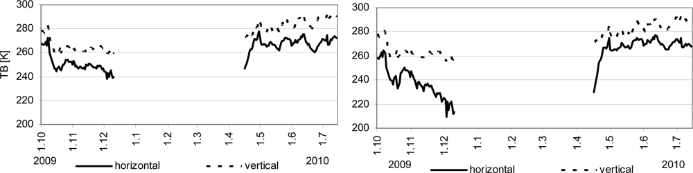
For the analysis of the radiometer data only the angles 50–65° were used, because of the increasing fraction of sky radiance detected at angles above 65° [12]. Systematic errors were corrected by referring all the temperatures to the measured zenith temperatures Tpzenith (p = h,v) [12]. For each incidence angle 2 measurements per hour were performed. Figure 7 shows the evolution of brightness temperatures over the experiment period for two angles and both horizontal and vertical polarizations.
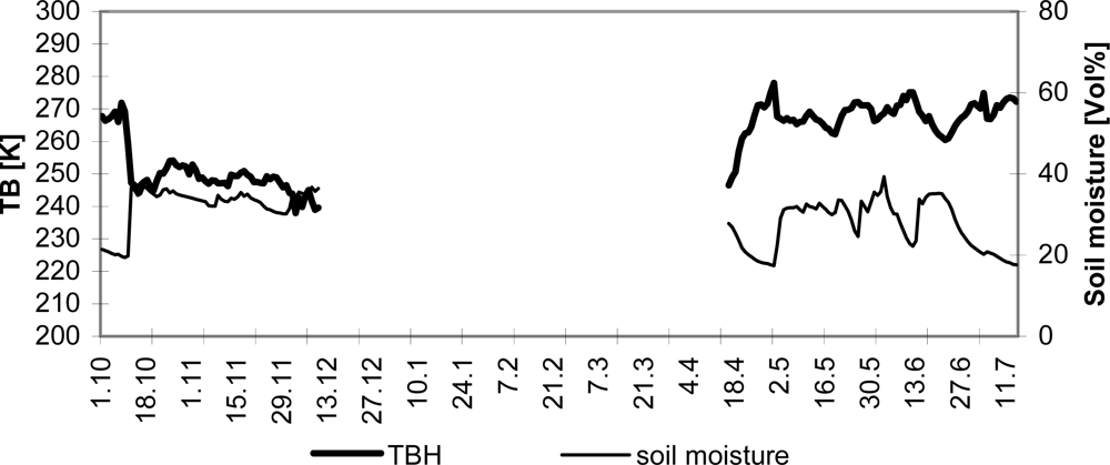
The data gap is due to technical problems during the freezing period. Because of the direct relationship between emission of radiation and water content of the soil, strongly connected to the dielectric properties, the radiometer signal reacts inversely to the development of soil moisture [31] as can be seen in Figure 8.
Next to the radiometer horn, thermal infrared measurements were performed with the IR radiometer Everest Interscience 4,000.4 ZH. This device is sensitive in the spectral range from 8 to 15 μm, the temperature range is 243–1,033 K and the accuracy is ±1% of reading [12]. These measurements were used for constantly detecting the physical temperature of the soil surface the radiometer is pointed at.
3. Model and Methods
3.1. Microwave Radiative Transfer Model
The microwave radiative transfer model L-MEB (L-Band Microwave Emission of the Biosphere) is used in this study to simulate the microwave emission of a vegetated surface at L-Band. A detailed description of the model physics is provided by [9], therefore only a brief overview is given here.
The basis of L-MEB is the Tau (τ)-Omega (ω) model [9], which simulates the overall brightness temperature TB of a natural surface. This simple radiative transfer model uses two parameters to characterize the land surface: the vegetation optical depth τ and the single scattering albedo ω. They are used to parameterize vegetation attenuation and scattering effects. In several studies, the τ-ω-model has usually been found to be an accurate approach to model the L-Band emission from a vegetation canopy [9].
Using that model, the overall emission from a two layer medium (soil and vegetation) is for each polarization (horizontal and vertical) the sum of the three terms soil emission attenuated (scattered and absorbed) by the vegetation layer, direct vegetation emission and vegetation emission reflected by the soil and attenuated again by the vegetation. It results in a polarized (p = h,v) brightness temperature (TBP):
where TC and TG are the vegetation and the effective soil temperatures, rGp is the soil reflectivity, γp the vegetation attenuation factor, expressed by the vegetation optical depth and ωp the vegetation single scattering albedo [9].
The effective temperature of the soil is composed of a contribution of signals from different soil layers in different depths. According to the sensing depth variation with soil moisture content, the soil moisture is also taken into account here [32]. Thus in L-MEB the following equation is used to parameterize TG:
TDeep here refers to the temperature at 50 cm and TSurf to the temperature at 2 cm depth. Note, that Equation (2) neglects multiple scattering effects within the soil layer [9]. The higher the soil moisture is, the smaller is the depth, the radiation signal originates from [12]. Accounting for this effect, Wigneron et al. [9] changed Equation (2), parameterizing the factor C as function of soil moisture as follows:
where SM is the soil moisture in a depth of 5cm, which has a strong influence on emission characteristics of a surface. W0 and bw0 are semi-empirical parameters according to textural properties. Wigneron et al. [9] use the values w0 = 0.3 m3/m3 and bw0 = 0.3 as default values in L-MEB.
The reflectivity rGp at the soil/atmosphere interface is dependent upon the dielectric properties of the soil, originating from the dielectric roughness that depends on soil moisture, temperature, salinity, texture and geometrical roughness [16]. Referring to [33], the dielectric roughness is a function of the dielectric permittivity εS and of surface roughness effects. For the lower frequency range (1–20 GHz), several models have been developed to relate εS to soil parameters such as moisture, bulk density or proportion of sand and clay. In L-MEB the model of DOBSON [34] or MIRONOV [35] is used to calculate εS. Freezing also affects εS seriously, but is not accounted for within this study [33].
In L-MEB the geometrical roughness is expressed through the parameters Hr (mean roughness), NH,V (polarization dependent roughness), and QR (frequency dependent roughness). The latter has no influence in the region of 1.4 GHz and thus is set to zero in L-MEB [30]. According to [30], there is an exponential relation between the standard deviation of heights of the soil surface s and Hr. According to that functional relation, for the case of the Puch experiment, the measured s in the field would correspond to a roughness parameter Hr of approximately 0.5.
In the L-Band the scattering effects, represented by the single scattering albedo ωp (where the subscript P stands for polarization) are generally found in the literature to be low. For most low vegetation types, ωp is below 0.05 [9]. The vegetation attenuation factor γp is mainly expressed by the vegetation optical depth τp through the equation
with τp as vegetation optical depth and θ as incidence angle. As presented in the following, τp is expressed as a function of the overall vegetation optical depth at nadir (θ = 0°).
τp is generally found to be linearly related to the total vegetation water content VWC [kg/m2], using the b-parameter. For calculation of the vegetation optical depth through τ = b × VWC, a value of b = 0.12 ± 0.03 was found to be representative for most agricultural crops.
Some results of previous studies showed a strong relationship between vegetation optical depth and LAI. Through this, and because of the relationship between LAI and VWC (R2 = 0.95 for fallow at SMOSREX [10]), it is possible to calculate the vegetation optical depth from LAI through the linear equation:
Although the calculation of the vegetation optical depth with the water content is assumed to be more stable, in this study we decided to retrieve τ from the LAI because the LAI can be derived on the global scale from satellite data which is important for the global application of SMOS.
3.2. Methods
Due to the lack of L-MEB parameterizations for rape in a first step the brightness temperature modeling ability of L-MEB over winter oilseed rape was tested by using the SMOS default parameters for Central European crops to parameterize L-MEB and compare the simulated with measured brightness temperatures. After that it was tried to develop a better L-MEB parameterization for the land use winter oilseed rape. In order to do that, a sensitivity study was conducted to find the parameters with the most pronounced effect on the modeling. Next, different parameter retrievals are performed to estimate the L-MEB parameters needed for a proper modeling. In the end, the soil moisture retrieval capabilities of the new parameterization are assessed.
To test the suitability of the SMOS default parameters for Central European crops that are also used in the SMOS L2 soil moisture retrieval algorithm (Table 3) [36] for the radiative transfer modeling over winter oilseed rape, L-MEB was used with the default parameters to model the brightness temperatures in a simple forward modeling approach. The results are compared with the measured brightness temperatures from the radiometer ELBARA II. To enable a comparison with other retrievals carried out later, L-MEB is also used to assess the soil moisture retrieval performance of the default parameters in a one parameter retrieval. The parameters in Table 3 correspond to the default values as described in [36] that are in accordance with the operational version of the SMOS L2 soil moisture processor. As the Hr value is implemented as a piecewise function of soil moisture in the SMOS L2 soil moisture processor, the Hr value in Table 3 corresponds to the maximum value of Hr that is being used in the processor.
The above mentioned continuous soil moisture measurements in 5 cm depth and the soil temperature measurements in 2 cm and 50 cm depth were used as input for the model together with the LAI measurements that were interpolated. The soil parameters and the air temperature that are needed for the modeling were also taken from the measurements described above.
To analyze which parameters affected the modeling result the most for our experiment, a sensitivity study was performed. Within this study, all the parameters mentioned above, were tested for their sensitivity to the modeling results in the forward modeling approach described above. As a result, the b-parameters controlling the vegetation optical depth τ, Hr characterizing the surface roughness and the single scattering albedo ω (only valid for the first period of the experiment) had a considerable impact on the modeling result. All the other parameters remained ‘default’ for the entire experiment.
Because of the afore mentioned structural difference of winter rape in early and late growing period which leads to a very different vegetation behavior at L-Band, the study handles the part before and after winter break separately. Due to data gaps in the radiometer data the winter break extends into April. The first period in 2009 is 71 days long and contains 39 vegetation days (mean-temperature >5 °C) while the second period in 2010 is 90 days long and contains 90 vegetation days.
The procedure for finding the best possible L-MEB parameterization for winter oilseed rape at the specific test site Puch was basically the same for both periods, with different results in each case. An iterative inversion approach was used to retrieve different combinations of L-MEB parameters from the multiangular ELBARA II measurements using different ground data sets as input. The procedure is outlined in the following:
At first a three parameter (3P)-retrieval is conducted with soil moisture, vegetation optical depth and roughness as free parameters while measured soil temperatures are used as input to L-MEB. The result is analysed and the retrieved parameters are compared to the ground measurements. Especially the relationship between measured LAI and VWC and retrieved vegetation optical depth as well as the relationship between retrieved roughness and measured roughness are investigated.
To establish a relationship between the retrieved vegetation optical depth and the measured LAI and VWC the b-parameters for this relationship were estimated by establishing a linear regression between measured LAI and VWC and the retrieved vegetation optical depth (see Equation (5)).
It is assumed that the new b-parameters and the mean value of the retrieved roughness parameter Hr can be treated as a possible new parameterization for L-MEB over winter oilseed rape in Puch. In the following steps this new parameterization is assessed.
The retrieved vegetation optical depth is compared to a calculated vegetation optical depth using the new b-parameters and interpolated values of measured LAI and VWC to see how well the new b-parameters are able to reproduce the retrieved vegetation optical depth.
The soil moisture retrieval capabilities of this parameterization is tested by comparing the retrieved soil moisture from a one parameter (1P)-retrieval (only soil moisture as free parameter; roughness fixed at the above mentioned mean value of retrieved roughness from the 3P-retrieval; vegetation optical depth calculated from the interpolated LAI measurements with the new b-parameters) to measured soil moisture.
As the roughness does not seem to be constant it is analyzed if there is a relationship between soil moisture and roughness by calculating a linear regression between measured soil moisture and retrieved roughness. This has been reported by different authors for grass [37,38].
To assess the influence of roughness on the soil moisture retrieval result two additional retrievals are carried out:
- A 1P-soil moisture retrieval where Hr is not constant but a function of measured soil moisture
- A two parameter (2P)-retrieval with soil moisture and roughness as free parameters
The performance of the different dielectric models of DOBSON and MIRONOV in the 3P-retrieval are compared as well as other authors found that the MIRONOV model is better under certain conditions than the DOBSON model which is currently the default model in the SMOS processor [30].
In the end the soil moisture retrieval capabilities of the new parameterization are summarized and the influence of the different parameters assessed.
4. Results and Discussion
4.1. SMOS Default Parameterization and Sensitivity Study
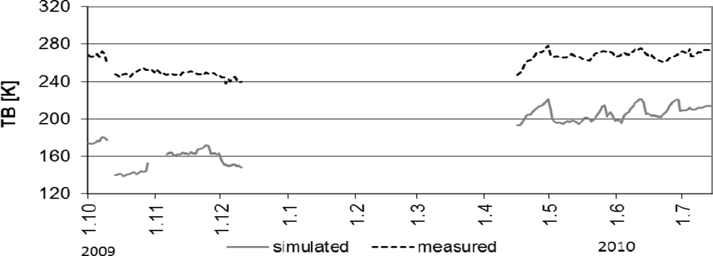
A comparison of the time series of measured and forward modeled brightness temperatures using the default parameters for crops shows that there is a considerable deviation between both data sets. Figure 9 shows the comparison for an incidence angle of 50°.
With root mean squared errors of 75.7 K for horizontal and 29.6 K for vertical polarization, there are considerable deviations between both time series. L-MEB severely underestimates the measurement when parameterized with the ‘SMOS default parameters’. When used for a 1-P soil moisture retrieval these parameters lead to RMSE values of 0.354 m3/m3 and 0.283 m3/m3 soil moisture for the first and second period respectively under the current conditions which is not satisfying.
The sensitivity study conducted to find the parameters that need to be changed revealed that vegetation and roughness parameterization have to be adapted to the specific features of winter oilseed rape at the location Puch. According to [9] the vegetation optical depth Tau is positively correlated to the brightness temperature, in the way, that an increasing Tau leads to an increase of the TB. To minimize the deviation between the measured and the retrieved TB, a new set of b-parameters had to be found for the land use winter oilseed rape. Another aspect which leads to an increase of the modeled value is an increase of the roughness condition, here in form of the parameter Hr [9]. For this reason, the vegetation optical depth (mainly the b-parameters) as well as the roughness conditions in form of the parameter Hr had to be adapted to the specific conditions of the test site.
A roughness parameter of Hr = 0.8 was found to produce good results. Another result of the sensitivity study was that the forward modeling approach delivers the best results for the early growing period when a single scattering albedo of 0.07 is used. As this value is also reported in literature for different crops [39] it was decided to use it throughout this study for the early growing period. The b-parameters that were found to produce best results lie in the order of b1 = 0.135 − 0.14 and b2 = 0.08 − 0.1.
With the above described insights it is possible to find parameterizations for L-MEB that enable forward modeling of the 50° brightness temperatures with an RMSE between 1.5 K and 7.1 K for both periods and both polarizations. If higher incidence angles are used (e.g., 70°) the RMSE increases to 24 K, as L-MEB is known to work less efficiently at high incidence angles. Therefore it is expected that the usage of several angles in a soil moisture retrieval from measured brightness temperatures will be able to produce reasonable results even if they will not be as good as the forward modeling results for 50°. It was not possible to model the periods before and after winter break with one set of parameters satisfyingly because of the afore mentioned difference in vegetation behavior at L-Band due to the structural difference of winter rape in both periods. Therefore the two periods are treated separately.
The sensitivity study was also used to find initial values and uncertainties for the parameters that produce best retrieval results. They are listed in Table 4.
4.2. Retrieval Results for Early Growing Period
The roughness and vegetation optical depth that were retrieved using the 3P-retrieval for the early growing period are shown in Figure 10.
A rise of the vegetation optical depth is visible for the first part of the period. A decrease in physical temperature leads to a decrease of plant vitality and thus to a decrease of vegetation optical depth in the second half. With the loss of plant vitality and VWC, the retrieved roughness seems to become smoother. The mean vegetation optical depth in this period is 0.27, the mean Hr is 0.71 which is of the same order as the value of 0.8 that was found in the sensitivity study but is considerably higher than the value around 0.5 that was estimated from the roughness measurements. The roughness seems to decrease slightly in the course of this period.
Referring to [9] there is a linear relationship between measured leaf area index (LAI) and vegetation optical depth. Equation 5 is used to calculate the two b-parameters from the linear regression between measured LAI and retrieved vegetation optical depth. The R² for this relationship is 0.6, the regression equation was τ = 0.12 × LAI + 0.08. Referring to Equation (5) that means: b1 = 0.12 and b2 = 0.08. It is important to mention that this regression is based on only four LAI measurements and therefore may not be very reliable. Nevertheless, these two b-parameters together with the mean retrieved Hr parameter are considered a possible extension to the L-MEB parameterization for winter oilseed rape in such an early growing stage and are evaluated in the following. The new parameterization is summarized in Table 3. Because of the lack of data, a relationship between VWC and vegetation optical depth could not be established.
A comparison between the retrieved vegetation optical depth and a calculated one using the measured LAI values together with the new b-parameters in Equation (5) is shown by Figure 10.
Both lines follow a similar trend even though the calculated Tau shows less variability, which is as expected due to the small amount of LAI measurements that have been interpolated for this comparison. The RMSE is 0.03. Calculated Tau values are only available after November 6 as this was the start of the LAI measurements.
A comparison between the retrieved and measured soil moisture is shown in Figure 11. The retrieved soil moisture follows the overall evolution of the measured soil moisture except on the first days of the experiment, but the variability is considerably higher in the retrieved soil moisture. This may be an indication that the radiometer “sees” a different, more dynamic, soil layer (e.g., 0–2 cm) than what is being measured by the TDR probes (5 cm horizontally). R2 for this comparison is 0.76 and the root mean squared error 0.057 m3/m3.
The soil moisture retrieval capabilities of the new parameterization are tested by retrieving soil moisture in a 1P-retrieval from the ELBARA measurements. Roughness is parameterized with a constant Hr value of 0.71 and the vegetation optical depth is calculated with the new b-parameters from interpolated LAI measurements. The resulting soil moisture can be seen in Figure 11 together with measured soil moisture and the retrieved soil moisture from the 3P-retrieval. R2 decreases to 0.33 and the RMSE increases to 0.086 m3/m3 for the comparison with the measured soil moisture. Obviously, the 1P-retrieval works considerably less well than the 3P-retrieval for soil moisture. One has to bear in mind that the retrievals that use a calculated Tau can only be performed for the time after 6 November as no LAI measurements are available before that. Therefore these comparisons are not as reliable as the period analyzed is relatively short. The retrieved soil moisture shows more variability than the measured one. All in all the measured soil moisture shows a very low dynamic after the first days of this period.
To study whether the changing roughness from the 3P-retrieval is dependent on soil moisture which has been reported earlier [37,38,40] and is also accounted for in the SMOS algorithm, the correlation between both datasets is calculated, the result is shown in Figure 12. With increasing soil moisture, Hr is decreasing.
If this linear regression is used to parameterize Hr as a function of soil moisture during a 1P-soil moisture retrieval, the result is very similar to the 1P-retrieval with constant Hr (see Table 5). The two Hr values have nearly the same evolution over time (not shown). If Hr is left free in a 2P-retrieval where soil moisture and Hr are retrieved the retrieved soil moisture follows very closely the evolution of the 3P-retrieved soil moisture (not shown) after November 6. Before that date no 2-P retrieval is possible due to a lack of LAI measurements. The RMSE is even lower than in the 3-P-retrieval but R² is considerably lower for the 2-P-retrieval which is probably due to the low soil moisture dynamic after November 6 (Table 5).
Table 5 summarizes the soil moisture retrieval results for the different retrievals carried out.
To test the influence of the dielectric model used in L-MEB the 3P-retrieval is also done with the MIRONOV dielectric model and compared to the above mentioned results produced with the DOBSON model. The effect is very small. The RMSE between modeled and simulated soil moisture is 0.004 m3/m3 higher (0.061 m3/m3) by using MIRONOV than that one by using DOBSON.
4.3. Retrieval Results for Late Growing Period
The late growing period is treated analogue to the early period. The difference is that the soil moisture is being retrieved from a surface, densely covered with winter oilseed rape plants. Plants with horizontally oriented, small leaves and low plant column density, are now turning to plants with vertical stems, leaves, flowers and later pods.
Figure 13 shows roughness and vegetation optical depth as retrieved during the 3P-retrieval together with soil moisture.
Vegetation optical depth shows an increase at the beginning which can be connected to vertical plant growth. The vegetation height increased from about 70 cm mid of April to 130 cm mid of May. Since that point of time no further vertical growth was detected. The soil roughness remains at a more or less constant level but tends to decrease slightly in the beginning. It is considerably higher than during the first period. The mean value of Hr is 0.93 and the vegetation optical depth totaled at a mean of 0.29.
Using Equation (5) the b-parameters for the second period were also estimated by using a linear regression between LAI and retrieved vegetation optical depth. The relationship shows an R² of 0.6 and the equation of the linear regression line reads as follows: τ = 0.09 × LAI + 0.08. Consequently b1 = 0.09 and b2 = 0.08. Because of having several VWC measurements in this period, it was also possible to establish a relationship between VWC and the retrieved vegetation optical depth, which provides a b-parameter of b = 0.07. Summarizing these results we get a possible L-MEB parameterization for the late growing period (Table 3).
Figure 14 compares the retrieved vegetation optical depth to that one calculated with the LAI and the water content of the plants (VWC) using the new b-parameters.
Throughout the whole period, the calculated vegetation optical depths generally follow the trend of the retrieved value. Here again the retrieved values show a higher variability. The deviation between the two calculated and the retrieved vegetation optical depth is similar but evolves differently over time. Both calculated Taus have their maximum at different points in time. The one calculated from VWC develops more smoothly.
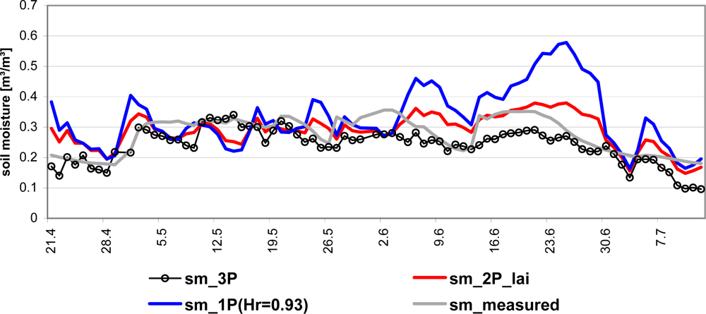
The soil moisture retrieval capabilities of the new parameterization for the late growing period are also tested by retrieving soil moisture in a 1P-retrieval from the ELBARA measurements. Roughness is parameterized with a constant Hr value of 0.93 (compare Figure 13) and the vegetation optical depth is calculated with the new b-parameters from interpolated LAI measurements. The resulting soil moisture can be seen in Figure 15 together with measured soil moisture and the retrieved soil moisture from the 3P-retrieval.
The picture is similar to the early growing period. The general trend of the soil moisture could be reproduced with the retrieved soil moisture but there are also considerable deviations. The 1P-retrieval results in a considerably higher RMSE and lower R2 (see Table 5) than the 3P-retrieval. Especially in June the retrieved soil moisture from the 1-P retrieval is considerably higher than the measured one.
To investigate if the roughness is dependant on soil moisture Figure 12 compares retrieved roughness to measured soil moisture. There is a weak relationship between both variables. With increasing soil moisture, roughness decreases, but only marginally from around 0.95 to around 0.92.
If the established linear regression is used to express the roughness as a function of soil moisture during a 1P-soil moisture retrieval no considerable improvement can be observed. While the RMSE decreases by 0.011 [m3/m3] the R2 decreases as well (Table 5). The evolution over time is very similar (not shown).
As a 2P-retrieval with soil moisture and roughness as free parameters leads to clearly improved results, it is probable that the roughness value leads to large errors if not left free (see Table 5 and Figure 15). Using VWC instead of LAI for the calculation of the vegetation optical depth does not lead to an improvement (Table 5). Especially in June, where the deviation between measured soil moisture and retrieved soil moisture from the 1P-retrieval is very high, the 2P-retrieval leads to considerable improvements. As the LAI reaches its maximum values at this time it is probable that vegetation effects lead to the high deviations between measured and retrieved soil moisture. As Tau is parameterized in the same way in both retrievals it is assumed that the parameter Hr incorporates some vegetation effects.
As in the early growing period the DOBSON dielectric model leads to better results than the MIRONOV model in the 3-P retrieval. The soil moisture RMSE increases by 0.020 m3/m3 to 0.069 m3/m3 when using MIRONOV instead of DOBSON.
4.4. Discussion of the Chosen Approach
One has to bear in mind that the dataset used for this study has two main drawbacks. Firstly the ELBARA data used was measured at angles between 50 and 65° which is only a rather small angle window at high sangles. L-MEB is known to be less efficient at high incidence angles. For that reason angles above 55° are filtered out in the SMOS soil moisture retrieval [36]. Secondly the soil moisture was measured in a depth of 5cm which may be lower than the sensing depth of the ELBARA as reported by [41]. Therefore the observed deviation between measured and retrieved soil moisture may include an error that is being made when one assumes that the ELBARA is sensing the soil moisture measured in 5cm depth. The rather high incidence angles at the edge of the region where soil moisture retrievals can still deliver satisfying results complicate things further.
In addition to that only a small number of LAI measurements during the early growing period makes it necessary to keep the uncertainties in mind that originate from this.
During the second period the vegetation optical depth is very high during the main growing season which decreases the soil moisture sensitivity of the ELBARA data. The VWC has values around 6 kg/m2 at this time.
When the results from the L-MEB modeling with the SMOS default parameters are discussed it has to be kept in mind that those parameters were only used as a starting point for the modeling due to the lack of a rape parameterization for L-MEB. If the conclusions drawn here are to be considered in the context of a satellite application several factors have to be considered that differ from point scale to satellite scale, e.g., the scale of the instrument footprint or the footprint heterogeneity.
5. Conclusions
A new parameterization for the radiative modeling of L-Band microwave emission from a rape field was developed. Significant differences were found between early and late rape development stages that led to the development of two different parameterizations for the two development stages.
It was especially important to adapt the roughness parameter Hr and the b-parameters to local conditions. In case of the early growing period the single scattering albedo has also been adapted. All other parameters have been taken from literature and correspond to the parameters used for the SMOS L2 processor.
Using the SMOS default parameterization in L-MEB for forward modeling of the microwave emission led to a clear offset in the order of 30 K−75 K for vertical and horizontal polarization respectively. This corresponds to a soil moisture retrieval RMSE above 0.28 m3/m3 in a 1-P retrieval.
It was not possible to find one parameterization that allowed satisfying microwave emission modeling results for the periods before and after winter for winter oilseed rape. Remarkable is the considerably increased roughness parameter Hr after winter as it would be expected that the soil becomes smoother in winter. This may be connected to the different development stages of the rape plants during the two periods. Apparently the roughness parameter Hr includes a vegetation dependant component. It was interesting to see that the retrieved values for the roughness parameter Hr lied consistently over the expected range that was found in studies over different crops and was estimated from measurements [9,30]. A value of 0.7–0.9 is considered a very rough soil by these studies, which was not observed in Puch. Other studies however found similar values of Hr [42] and also conclude that a constant value of Hr or a simple linear regression with soil moisture could lead to significant retrieval errors due to a dynamic roughness parameter. Panciera et al. [42] also concludes that a dielectric component in the microwave roughness which is related to soil moisture microscale heterogeneity might be responsible for this effect.
It does not seem to be possible to establish a parameterization for L-MEB that allows a satisfying 1P-soil moisture retrieval from the ELBARA data described above under the apparent conditions in Puch. As a 2P-retrieval with soil moisture and roughness as free parameters leads to clearly improved results the roughness parameterization seems to be responsible for a considerable part of the encountered problems. The uncertainties in the vegetation optical depth modeling, that are clearly existent seem to have a smaller impact on the soil moisture retrieval. Another aspect that can explain the retrieval quality is the fact that no angles below 50° were available which is not ideal as L-MEB is known to be less efficient at high incidence angles. The observed relationship between soil moisture and Hr does not help to improve soil moisture retrievals considerably.
Still, the 3P-retrievals show that it is possible to retrieve soil moisture with an RMSE in the order of 0.049–0.057 m3/m3 and a R2 of 0.70–0.76 with multiangular ELBARA II data above 50° if the roughness and vegetation optical depth are left free, which is promising. When doing a 2P retrieval (soil moisture and roughness free) with the usage of the newly found b-parameters to calculate vegetation optical depth from LAI the retrieved soil moisture shows RMSE values of around 0.045–0.051 m3/m3 with R² values of 0.33 and 0.40 for early and late growing period respectively.
Under the reported conditions the DOBSON dielectric model performs better than the MIRONOV model.
As this study is the first to the authors’ knowledge that has studied the passive microwave emission from rape fields, the gained insights into the radiative transfer modeling over rape fields can surely add to the existing knowledge in the field of passive microwave remote sensing over different crops.
Acknowledgments
The authors wish to acknowledge the contributions of the students of the University of Munich helping with the in situ measurements and the assistance given by Timo Gebhardt in the operation of the instrument and the data processing. The authors would like to thank J.-P. Wigneron for making the model L-MEB available. The ELBARA instrument was kindly provided by ESA. Meteorological data as well as technical and logistical support was kindly provided by the Bavarian State Research Center for Agriculture, Versuchsstation Puch (Heiles) and Department Meteorology (Kerscher), which is gratefully acknowledged. The authors would like to thank the reviewers for their time and valuable comments which helped improve the paper. This work has been funded by the German Federal Ministry of Economics and Technology through the German Aerospace Center (DLR, 50 EE 0731) which is gratefully acknowledged.
References
- Jung, M.; Reichstein, M.; Ciais, P.; Seneviratne, S.I.; Sheffield, J.; Goulden, M.L.; Bonan, G.; Cescatti, A.; Chen, J.; de Jeu, R.; et al. Recent decline in the global land evapotranspiration trend due to limited moisture supply. Nature 2010, 467, 951–954. [Google Scholar]
- Kerr, Y.H.; Waldteufel, P.; Wigneron, J.-P.; Martinuzzi, J.-M.; Font, J.; Berger, M. Soil moisture retrieval from space: The Soil Moisture and Ocean Salinity (SMOS) mission. IEEE Trans. Geosci. Remote Sens 2001, 39, 1729–1735. [Google Scholar]
- Entekhabi, D.; Asrar, G.R.; Betts, A.K.; Beven, K.J.; Bras, R.L.; Duffy, C.J.; Dunne, T.; Koster, R.D.; Lettenmaier, D.P.; Mclaughlin, D.B.; et al. An agenda for land-surface hydrology research and a call for the second international hydrological decade. Bull. Am. Meteorol. Soc 1999, 80, 2043–2057. [Google Scholar]
- Wagner, W.; Naeimi, V.; Scipal, K.; de Jeu, R.; Martínez-Fernández, J. Soil moisture from operational meteorological satellites. Hydrogeol. J 2007, 15, 121–131. [Google Scholar]
- Aires, F.; Prigent, C.; Rossow, W.B. Sensitivity of satellite microwave and infrared observations to soil moisture at a global scale: 2. Global statistical relationships. J. Geophys. Res 2005, 110, D11103. [Google Scholar]
- Loew, A.; Ludwig, R.; Mauser, W. Derivation of surface soil moisture from ENVISAT ASAR wide swath and image mode data in agricultural areas. IEEE Trans. Geosci. Remote Sens 2006, 44, 889–899. [Google Scholar]
- Mauser, W.; Rombach, M.; Bach, H.; Demircan, A.; Kellndorfer, J. Determination of spatial and temporal soil-moisture development using multitemporal ERS-1 data. Proc. SPIE 1995, 2314, 502–515. [Google Scholar]
- Wagner, W.; Blöschl, G.; Pampaloni, P.; Calvet, J.-C.; Bizzarri, B.; Wigneron, J.-P.; Kerr, Y. Operational readiness of microwave remote sensing of soil moisture for hydrologic applications. Nord. Hydrol 2007, 38, 1–20. [Google Scholar]
- Wigneron, J.P.; Kerr, Y.; Waldteufel, P.; Saleh, K.; Escorihuela, M.J.; Richaume, P.; Ferrazzoli, P.; de Rosnay, P.; Gurney, R.; Calvet, J.C.; et al. L-band Microwave Emission of the Biosphere (L-MEB) Model: Description and calibration against experimental data sets over crop fields. Remote Sens. Environ 2007, 107, 639–655. [Google Scholar]
- de Rosnay, P.; Calvet, J.-C.; Kerr, Y.; Wigneron, J.-P.; Lemaître, F.; Escorihuela, M.J.; Sabater, J.M.; Saleh, K.; Barrié, J.; Bouhours, G.; et al. SMOSREX: A long term field campaign experiment for soil moisture and land surface processes remote sensing. Remote Sens. Environ 2006, 102, 377–389. [Google Scholar]
- Grant, J.P.; Wigneron, J.P.; Van de Griend, A.A.; Kruszewski, A.; Søbjærg, S.S.; Skou, N. A field experiment on microwave forest radiometry: L-band signal behaviour for varying conditions of surface wetness. Remote Sens. Environ 2007, 109, 10–19. [Google Scholar]
- Schwank, M.; Matzler, C.; Guglielmetti, M.; Fluhler, H. L-band radiometer measurements of soil water under growing clover grass. IEEE Trans. Geosci. Remote Sens 2005, 43, 2225–2237. [Google Scholar]
- Schwank, M.; Stahli, M.; Wydler, H.; Leuenberger, J.; Matzler, C.; Fluhler, H. Microwave L-band emission of freezing soil. IEEE Trans. Geosci. Remote Sens 2004, 42, 1252–1261. [Google Scholar]
- Loew, A.; Schwank, M.; Schlenz, F. Assimilation of an L-band microwave soil moisture proxy to compensate for uncertainties in precipitation data. IEEE Trans. Geosci. Remote Sens 2009, 47, 2606–2616. [Google Scholar]
- Loew, A.; Schwank, M. Calibration of a soil moisture model over grassland using L-band microwave radiometry. Int. J. Remote Sens 2010, 31, 5163–5177. [Google Scholar]
- Schwank, M.; Wiesmann, A.; Werner, C.; Mätzler, C.; Weber, D.; Murk, A.; Völksch, I.; Wegmüller, U. ELBARA II, An L-band radiometer system for soil moisture research. Sensors 2009, 10, 584–612. [Google Scholar]
- Cano, A.; Saleh, K.; Wigneron, J.-P.; Antolín, C.; Balling, J.; Kerr, Y.; Kruszewski, A.; Millán-Scheiding, C.; Søbjærg, S.; Skou, N. The SMOS Mediterranean Ecosystem L-Band characterisation EXperiment (MELBEX-I) over natural shrubs. Remote Sens. Environ 2010, 114, 844–853. [Google Scholar]
- Rautiainen, K.; Lemmetyinen, J.; Pulliainen, J.; Vehviläinen, J.; Drusch, M.; Kontu, A.; Kainulainen, J.; Seppänen, J. L-Band radiometer observations of soil processes in boreal and sub-arctic environments. IEEE Trans. Geosci. Remote Sens 2011, in press.. [Google Scholar]
- Schlenz, F.; Gebhardt, T.; Loew, A.; Marzahn, P.; Mauser, W. L-Band Radiometer Experiment in the SMOS Test Site Upper Danube. Proceedings of EGU General Assembly 2010, Vienna, Austria, 2–7 May 2010; p. 9677.
- FNR e.V. Jahresbericht 2009/2010; Fachagentur Nachwachsende Rohstoffe e.V. (FNR): Gülzow-Prüzen, Germany, 2010.
- Dall’Amico, J.T.; Schlenz, F.; Loew, A.; Mauser, W.; Kainulainen, J.; Balling, J.; Bouzinac, C. Airborne and ground campaigns in the Upper Danube Catchment: Data sets for calibration, validation and downscaling of SMOS data. IEEE Trans. Geosci. Remote Sens 2011. submitted. [Google Scholar]
- Delwart, S.; Bouzinac, C.; Wursteisen, P.; Berger, M.; Drinkwater, M.; Martin-Neira, M.; Kerr, Y.H. SMOS Validation and the COSMOS Campaigns. IEEE Trans. Geosci. Remote Sens 2008, 46, 695–704. [Google Scholar]
- Teuling, A.J.; Hupet, F.; Uijlenhoet, R.; Troch, P.A. Climate variability effects on spatial soil moisture dynamics. Geophys. Res. Lett 2007, 34, L06406. [Google Scholar]
- LI-COR, Inc. LAI-2000 Plant Canopy Analyzer: Instruction Manual; LI-COR, Inc.: Lincoln, NL, USA, 2003. [Google Scholar]
- Behrens, T.; Diepenbrock, W. Using digital image analysis to describe canopies of winter oilseed rape (Brassica napus L.) during vegetative developmental stages. J. Agron. Crop Sci 2006, 192, 295–302. [Google Scholar]
- Rieke-Zapp, D.H.; Rosenbauer, R.; Schlunegger, F. A photogrammetric surveying method for field applications. Photogramm. Rec 2009, 24, 5–22. [Google Scholar]
- Marzahn, P.; Rieke-Zapp, D.; Ludwig, R. Assessment of soil surface roughness statistics for microwave remote sensing applications using a simple photogrammetric acquisition system. ISPRS 2011. submitted.. [Google Scholar]
- Taconet, O.; Ciarletti, V. Estimating soil roughness indices on a ridge-and-furrow surface using stereo photogrammetry. Soil Till. Res 2007, 93, 64–76. [Google Scholar]
- Marzahn, P.; Ludwig, R. On the derivation of soil surface roughness from multi parametric PolSAR data and its potential for hydrological modeling. Hydrol. Earth Syst. Sci 2009, 13, 381–394. [Google Scholar]
- Wigneron, J.P.; Chanzy, A.; Kerr, Y.H.; Lawrence, H.; Shi, J.; Escorihuela, M.J.; Mironov, V.; Mialon, A.; Demontoux, F.; de Rosnay, P.; Saleh-Contell, K. Evaluating an improved parameterization of the soil emission in L-MEB. IEEE Trans. Geosci. Remote Sens 2011, 49, 1177–1189. [Google Scholar]
- Woodhouse, I.H. Introduction to Microwave Remote Sensing; Taylor and Francis: London, UK, 2006. [Google Scholar]
- Holmes, T.R.H.; de Rosnay, P.; de Jeu, R.; Wigneron, R.J.P.; Kerr, Y.; Calvet, J.C.; Escorihuela, M.J.; Saleh, K.; Lemaître, F. A new parameterization of the effective temperature for L-band radiometry. Geophys. Res. Lett 2006, 33, L07405. [Google Scholar]
- Mätzler, C. Thermal Microwave Radiation. Applications for Remote Sensing; Institution of Engineering and Technology: London, UK, 2006. [Google Scholar]
- Dobson, M.C.; Ulaby, F.T.; Hallikainen, M.T.; El-Rayes, M.A. Microwave dielectric behavior of wet soil-Part II: Dielectric mixing models. IEEE Trans. Geosci. Remote Sens 1985, GE-23. 35–46. [Google Scholar]
- Mironov, V.; Bobrov, P. Spectroscopic microwave dielectric model of moist soils. In Advances in Geoscience and Remote Sensing; Jedlovec, G., Ed.; InTech: Vukovar, Croatia, 2009; pp. 279–302. [Google Scholar]
- Kerr, Y.; Waldteufel, P.; Richaume, P.; Davenport, P.; Ferrazzoli, P.; Wigneron, J.-P. SMOS Level 2 Processor Soil Moisture Algorithm Theoretical Basis Document (ATBD) V 3.5; CBSA, UoR, TV and INRA: Toulouse, France, 2011. [Google Scholar]
- Saleh, K.; Kerr, Y.H.; Richaume, P.; Escorihuela, M.J.; Panciera, R.; Delwart, S.; Boulet, G.; Maisongrande, P.; Walker, J.P.; Wursteisen, P.; Wigneron, J.P. Soil moisture retrievals at L-band using a two-step inversion approach (COSMOS/NAFE'05 Experiment). Remote Sens. Environ 2009, 113, 1304–1312. [Google Scholar] [Green Version]
- Panciera, R.; Walker, J.P.; Kalma, J.D.; Kim, E.J.; Saleh, K.; Wigneron, J.-P. Evaluation of the SMOS L-MEB passive microwave soil moisture retrieval algorithm. Remote Sens. Environ 2009, 113, 435–444. [Google Scholar]
- Van de Griend, A.A.; Wigneron, J.P. On the measurement of microwave vegetation properties: Some guidelines for a protocol. IEEE Trans. Geosci. Remote Sens 2004, 42, 2277–2289. [Google Scholar]
- Escorihuela, M.J.; Kerr, Y.H.; de Rosnay, P.; Wigneron, J.P.; Calvet, J.C.; Lemaitre, F. A simple model of the bare soil microwave emission at L-band. IEEE Trans. Geosci. Remote Sens 2007, 45, 1978–1987. [Google Scholar]
- Escorihuela, M.J.; Chanzy, A.; Wigneron, J.P.; Kerr, Y.H. Effective soil moisture sampling depth of L-band radiometry: A case study. Remote Sens. Environ 2010, 114, 995–1001. [Google Scholar] [Green Version]
- Panciera, R.; Walker, J.P.; Merlin, O. Improved understanding of soil surface roughness parameterization for L-band passive microwave soil moisture retrieval. IEEE Geosci. Remote Sens. Lett 2009, 6, 625–629. [Google Scholar]
Figure 1.
The Upper Danube catchment in Europe; the radiometer test site is marked with a circle.
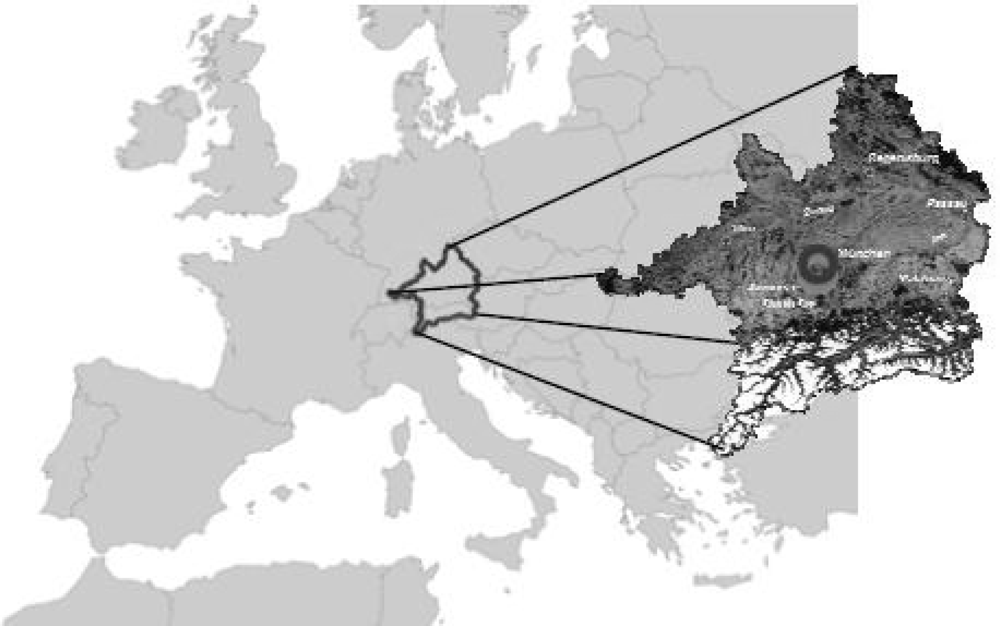
Figure 2.
Radiometer ELBARA II with angle of aperture α, incidence angle θ and the two halfaxes a and b of the elliptical footprint on the left; location of ground measurements (LAI and handheld soil moisture (FDR) inside the field of view (FOV), vegetation water content (VWC) outside the FOV; soil moisture and soil temperature stations for both fields are located to the right of the radiometer, the meteorological station to the left of the radiometer.

Figure 3.
Daily soil moisture measured at a depth of 5 cm and precipitation as daily sum for the whole campaign period; the data gaps are due to technical problems during winter-time.
Figure 3.
Daily soil moisture measured at a depth of 5 cm and precipitation as daily sum for the whole campaign period; the data gaps are due to technical problems during winter-time.

Figure 4.
Development of vegetation water content and leaf area index for the duration of the experiment.
Figure 4.
Development of vegetation water content and leaf area index for the duration of the experiment.

Figure 5.
Photographs of the winter rape canopy demonstrating stages of phenology at the beginning of October (top left), middle of November(top centre) and middle of December (top right) as well as May (bottom left) and July (bottom right).
Figure 5.
Photographs of the winter rape canopy demonstrating stages of phenology at the beginning of October (top left), middle of November(top centre) and middle of December (top right) as well as May (bottom left) and July (bottom right).

Figure 6.
Digital elevation model of a roughness measurement performed in October 2009, clearly visible is the tractor track on the right. The heights are relative to the lower edge of the scaffold.
Figure 6.
Digital elevation model of a roughness measurement performed in October 2009, clearly visible is the tractor track on the right. The heights are relative to the lower edge of the scaffold.
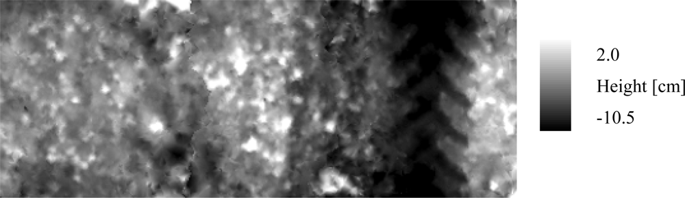
Figure 7.
Measured ELBARA brightness temperatures (TB) for angle 50° (left) and 65° (right) for both vertical and horizontal polarization.
Figure 7.
Measured ELBARA brightness temperatures (TB) for angle 50° (left) and 65° (right) for both vertical and horizontal polarization.

Figure 8.
Development of TB and soil moisture in 5 cm depth − 50°, horizontal polarisation.

Figure 9.
Comparison between simulated and measured TB on the basis of using the standard parameters according to literature—horizontal polarization.
Figure 9.
Comparison between simulated and measured TB on the basis of using the standard parameters according to literature—horizontal polarization.

Figure 10.
Development of vegetation optical depth at NADIR (tau_3P) and roughness parameter Hr (Hr _3P) as a result of a 3P-retrieval. Also shown is the calculated Tau (tau_calc).
Figure 10.
Development of vegetation optical depth at NADIR (tau_3P) and roughness parameter Hr (Hr _3P) as a result of a 3P-retrieval. Also shown is the calculated Tau (tau_calc).
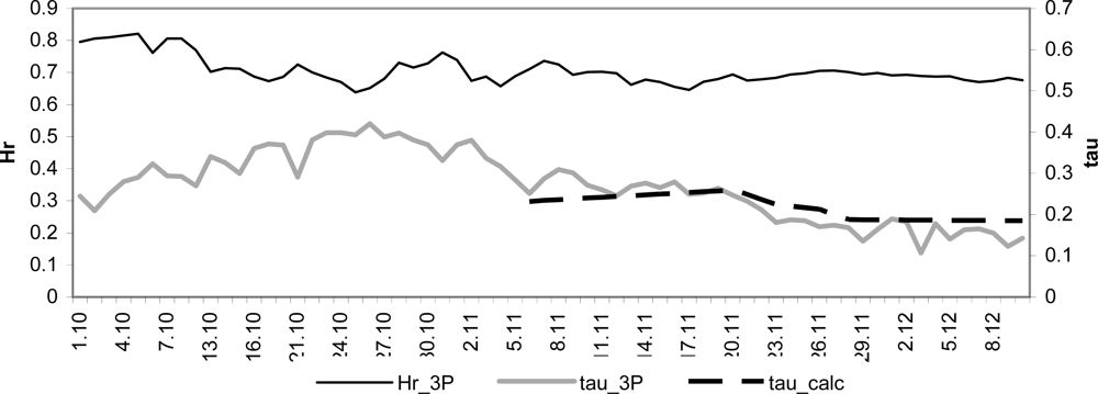
Figure 11.
Comparison between the soil moisture of the 3P-retrieval (sm_3P), the 1P-retrieval (sm_1P(Hr = 0.71)) with a constant value of Hr = 0.71 and the measured soil moisture at the location Puch.
Figure 11.
Comparison between the soil moisture of the 3P-retrieval (sm_3P), the 1P-retrieval (sm_1P(Hr = 0.71)) with a constant value of Hr = 0.71 and the measured soil moisture at the location Puch.
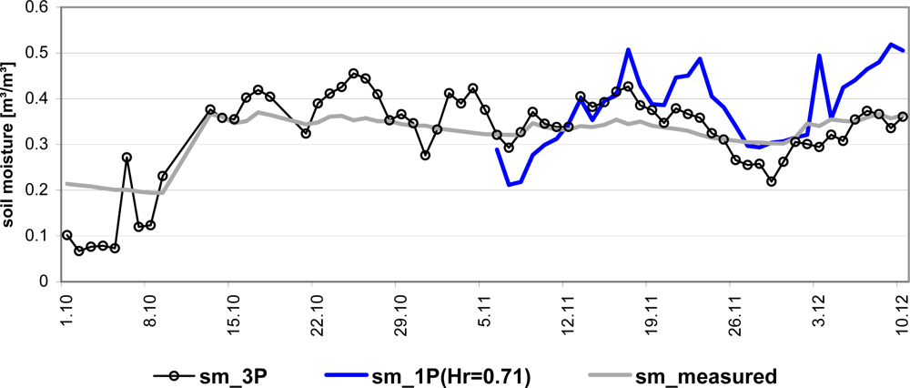
Figure 12.
Correlation between measured soil moisture and retrieved roughness parameter Hr for early (left) and late (right) growing period.
Figure 12.
Correlation between measured soil moisture and retrieved roughness parameter Hr for early (left) and late (right) growing period.
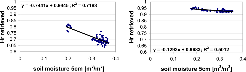
Figure 13.
Development of retrieved vegetation optical depth (tau_3P) and roughness parameter Hr (hr_3P).
Figure 13.
Development of retrieved vegetation optical depth (tau_3P) and roughness parameter Hr (hr_3P).
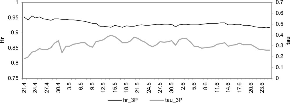
Figure 14.
Comparison between calculated vegetation optical depth on the basis of water content (tau_calc_vwc) or LAI (tau_calc_lai) and tau retrieved (tau_3P).
Figure 14.
Comparison between calculated vegetation optical depth on the basis of water content (tau_calc_vwc) or LAI (tau_calc_lai) and tau retrieved (tau_3P).
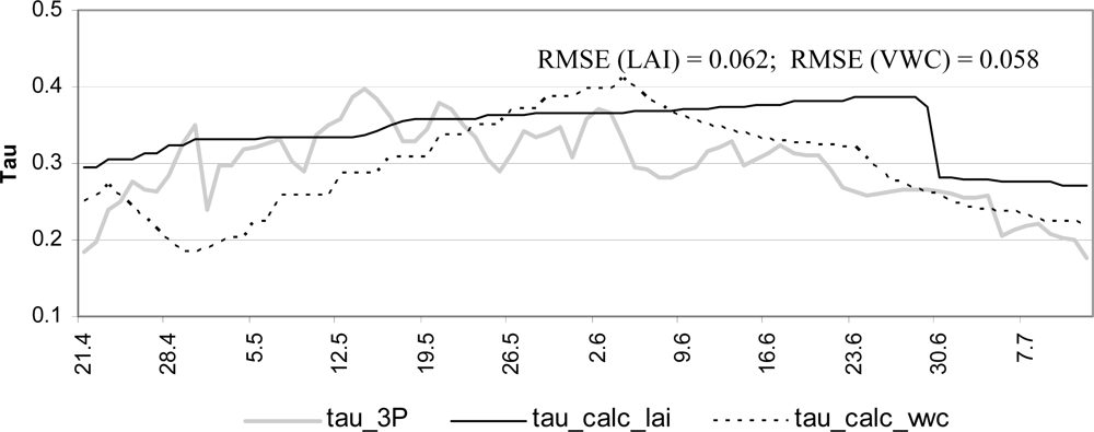
Figure 15.
Comparison between the soil moisture of the 3P-retrieval (sm_3P), the 1P-retrieval (sm_1P(Hr =0.93)) with a constant value of Hr = 0.93, the 2P-retrieval with tau calculated from LAI measurements(sm_2P_lai) and the measured soil moisture at the location Puch.
Figure 15.
Comparison between the soil moisture of the 3P-retrieval (sm_3P), the 1P-retrieval (sm_1P(Hr =0.93)) with a constant value of Hr = 0.93, the 2P-retrieval with tau calculated from LAI measurements(sm_2P_lai) and the measured soil moisture at the location Puch.

| Time | s [cm] |
|---|---|
| September 2009 | 1.161 |
| March 2010 | 1.005 |
| September 2010 | 1.312 |
| Incidence Angle [°] | FOV Length [m] | FOV Width [m] | FOV Area [m2] |
|---|---|---|---|
| 50 | 10.41 | 4.78 | 38.92 |
| 55 | 12.04 | 5.2 | 49.19 |
| 60 | 13.82 | 6.82 | 74.06 |
| 65 | 21.51 | 7.46 | 125.74 |
| 70 | 41.91 | 10.32 | 340.41 |
Table 3.
The different parameterizations used for L-band microwave emission of the biosphere (L-MEB) in this study. The first one corresponds to the Soil Moisture and Ocean Salinity (SMOS) default parameterization for Central European Crops, the other two have been developed within this study for the period before (early period) and after winter (late period).
| Parameter | w0/bw0 | tth/ttv | ωh/ωv | Hr | NH | Nv | Qr | b1 | b2 | b |
|---|---|---|---|---|---|---|---|---|---|---|
| SMOS default | 0.3/0.3 | 1/1 | 0/0 | 0.1 | 2 | 0 | 0 | 0.06 | 0 | - |
| Early period | 0.3/0.3 | 1/1 | 0.07/0 | 0.71 | 0 | −1 | 0 | 0.12 | 0.08 | - |
| Late period | 0.3/0.3 | 1/1 | 0/0 | 0.93 | 0 | −1 | 0 | 0.09 | 0.08 | 0.07 |
Table 4.
The initial values (and standard deviations) that are used for all the retrievals within this study for the retrieved parameters soil moisture, roughness parameter HR and vegetation optical depth.
| Soil moisture [m3/m3] | HR [-] | Vegetation optical depth [-] | |
|---|---|---|---|
| Early period | 0.3 (0.1) | 0.8 (0.1) | 0.2 (1.0) |
| Late period | 0.35 (0.1) | 0.8 (0.1) | 0.3 (1.0) |
Table 5.
Results from different soil moisture retrievals for the early and late growing period. During the 3P-retrieval soil moisture, tau and Hr are free parameters. Soil moisture and Hr are free in both 2P-retrievals while for one tau is calculated from LAI (2P(sm; Hr)_lai) and for the other tau is calculated from VWC (2P(sm; Hr)_vwc). Two different 1P-retrievals with soil moisture as free parameter have been carried out. One with a constant Hr value (1P(Hr = 0.xx)) and one with Hr parameterized as a function of soil moisture (1P(Hr = f(sm))).
| Period | Retrieval | R2 | RMSE [m3/m3] | Gain | Offset |
|---|---|---|---|---|---|
| Early | 3P(sm;tau; Hr) | 0.76 | 0.057 | 1.7 | 0.21 |
| 2P(sm; Hr))_lai | 0.33 | 0.045 | 1.61 | −0.21 | |
| 1P(Hr =0.71) | 0.33 | 0.086 | 2.57 | −0.48 | |
| 1P(Hr =f(sm)) | 0.22 | 0.078 | 1.88 | −0.22 | |
| Late | 3P(sm;tau;Hr) | 0.70 | 0.049 | 0.80 | 0.02 |
| 2P(sm; Hr))_lai | 0.40 | 0.051 | 0.60 | 0.12 | |
| 2P(sm; Hr)_vwc | 0.35 | 0.076 | 0.84 | 0 | |
| 1P (Hr =0.93) | 0.16 | 0.108 | 0.69 | 0.14 | |
| 1P(Hr =f(sm)) | 0.14 | 0.097 | 0.59 | 0.15 | |
Share and Cite
MDPI and ACS Style
Schlenz, F.; Fallmann, J.; Marzahn, P.; Loew, A.; Mauser, W. Characterization of Rape Field Microwave Emission and Implications to Surface Soil Moisture Retrievals. Remote Sens. 2012, 4, 247-270. https://doi.org/10.3390/rs4010247
AMA Style
Schlenz F, Fallmann J, Marzahn P, Loew A, Mauser W. Characterization of Rape Field Microwave Emission and Implications to Surface Soil Moisture Retrievals. Remote Sensing. 2012; 4(1):247-270. https://doi.org/10.3390/rs4010247
Chicago/Turabian StyleSchlenz, Florian, Joachim Fallmann, Philip Marzahn, Alexander Loew, and Wolfram Mauser. 2012. "Characterization of Rape Field Microwave Emission and Implications to Surface Soil Moisture Retrievals" Remote Sensing 4, no. 1: 247-270. https://doi.org/10.3390/rs4010247