Scene Classification Based on a Deep Random-Scale Stretched Convolutional Neural Network


State Key Laboratory of Information Engineering in Surveying, Mapping and Remote Sensing, Wuhan University, Wuhan 430079, China
*
Author to whom correspondence should be addressed.
Remote Sens. 2018, 10(3), 444; https://doi.org/10.3390/rs10030444
Submission received: 10 January 2018
/
Revised: 10 February 2018
/
Accepted: 19 February 2018
/
Published: 12 March 2018
(This article belongs to the Special Issue Deep Learning for Remote Sensing)
Abstract
:With the large number of high-resolution images now being acquired, high spatial resolution (HSR) remote sensing imagery scene classification has drawn great attention but is still a challenging task due to the complex arrangements of the ground objects in HSR imagery, which leads to the semantic gap between low-level features and high-level semantic concepts. As a feature representation method for automatically learning essential features from image data, convolutional neural networks (CNNs) have been introduced for HSR remote sensing image scene classification due to their excellent performance in natural image classification. However, some scene classes of remote sensing images are object-centered, i.e., the scene class of an image is decided by the objects it contains. Although previous methods based on CNNs have achieved comparatively high classification accuracies compared with the traditional methods with handcrafted features, they do not consider the scale variation of the objects in the scenes. This makes it difficult to directly utilize CNNs on those remote sensing images belonging to object-centered classes to extract features that are robust to scale variation, leading to wrongly classified scene images. To solve this problem, scene classification based on a deep random-scale stretched convolutional neural network (SRSCNN) for HSR remote sensing imagery is proposed in this paper. In the proposed method, patches with a random scale are cropped from the image and stretched to the specified scale as the input to train the CNN. This forces the CNN to extract features that are robust to the scale variation. Furthermore, to further improve the performance of the CNN, a robust scene classification strategy is adopted, i.e., multi-perspective fusion. The experimental results obtained using three datasets—the UC Merced dataset, the Google dataset of SIRI-WHU, and the Wuhan IKONOS dataset—confirm that the proposed method performs better than the traditional scene classification methods.

1. Introduction
Remote sensing image scene classification, which involves dividing images into different categories without semantic overlap [1], has recently drawn great attention due to the increasing availability of high-resolution remote sensing data. However, it is difficult to achieve satisfactory results in scene classification directly based on low-level features, such as the spectral, textural, and geometrical attributes, because of the so-called “semantic gap” between low-level features and high-level semantic concepts, which is caused by the object category diversity and the distribution complexity in the scene.
To overcome the semantic gap, many different scene classification techniques have been proposed. The bag-of-visual-words (BoVW) model, which is derived from document classification in text analysis, is one of the most popular methods in scene classification. In consideration of the spatial information loss, many BoVW extensions have been proposed [2,3,4,5,6,7,8]. Spatial pyramid co-occurrence [2] was proposed to compute the co-occurrences of visual words with respect to “spatial predicates” over a hierarchical spatial partitioning of an image, to capture both the absolute and relative spatial arrangement of the words. The topic model [9,10,11,12,13,14,15,16], as used for document modeling, text classification, and collaborative filtering, is another popular model for scene classification. P-LDA and F-LDA [9] were proposed based on the latent Dirichlet allocation (LDA) model for scene classification. Because of the weak representative power of a single feature, multifeature fusion has also been adopted in recent years. The semantic allocation level (SAL) multifeature fusion strategy based on the probabilistic topic model (PTM) (SAL-PTM) [10] was proposed to combine three complementary features, i.e., the spectral, texture, and scale-invariant feature transform (SIFT) features. However, in the traditional methods, feature representation plays a big role and involves low-level feature selection and middle-level feature design. As a lot of prior information is required, this limits the application of these methods in other datasets or other fields.
To automatically learn features from the data directly, without low-level feature selection and middle-level feature design, a number of methods based on deep learning have recently been proposed. A new branch of machine learning theory—deep learning—has been widely studied and applied to facial recognition [17,18,19,20], scene recognition [21,22], image super-resolution [23], video analysis [24], and drug discovery [25]. Differing from the traditional feature extraction methods, deep learning, as a feature representation learning method, can directly learn features from raw data without prior information. In the remote sensing field, deep learning has also been studied for hyperspectral pixel classification [26,27,28,29], object detection [30,31,32] and scene classification [33,34,35,36,37,38,39,40,41]. The auto-encoder [37] was the first deep learning method introduced to remote sensing image scene classification, combining a sample selection strategy based on saliency with the auto-encoder to extract features from the raw data, achieving a better classification accuracy than the traditional remote sensing image scene classification methods such as BoVW and LDA. The highly efficient “enforcing lifetime and population sparsity” (EPLS) algorithm, another sparse strategy, was introduced into the auto-encoder to ensure two types of feature sparsity: population and lifetime sparsity [38]. Zou et al. [39] translated the feature selection problem into a feature reconstruction problem based on a deep belief network (DBN) and proposed a deep learning-based method, where the features learned by the DBN are eliminated once their reconstruction errors exceed the threshold. Although the auto-encoder-based algorithms can acquire excellent classification accuracies when compared with the traditional methods, they do need pre-training, and can be regarded as convolutional neural networks (CNNs) in practice. Zhang et al. [40] combined multiple CNN models based on boosting theory, achieving a better accuracy than the auto-encoder methods.
However, most previous methods based on deep learning model such as CNN took images with single scale for training, by cropping the fixed scale patches from image or resizing the image to fixed single and did not consider the object scale variation problem in image caused by the altitude or angle change of the sensor, etc. The features extracted by these methods are not robust to the object scale, leading to unsatisfactory remote sensing image scene classification results. An example of scale variation of object is given in Figure 1, where the scale of the storage tank and airplane changed a lot which may be caused by the altitude or angle change of the sensor.
In order to solve the object scale variation problem, scene classification based on a deep random-scale stretched convolutional neural network (SRSCNN) is proposed in this paper. In SRSCNN, patches with a random scale are cropped from the image, and patch stretching is applied, which simulates the object scale variation to ensure that the CNN learns robust features from the remote sensing images.
The major contributions of this paper are as follows:
(1) The random spatial scale stretching strategy. In SRSCNN, random spatial scale stretching is proposed to solve the problem of the dramatic scale variation of objects in the scene. Some objects such as airplanes and storage tanks are very important in remote sensing image scene classification. However, the object scale variation can lead to weak feature representation for some scenes, which in turn leads to wrong classification. In order to solve this problem, the assumption that the object scale variation satisfies a uniform or a Gaussian distribution is adopted in this paper, and the strategy of cropping patches with a random scale following a certain distribution is applied to simulate the object variation in the scene, forcing the model to extract features that are robust to scale variation.
(2) The robust scene classification strategy. To fuse the information from different-scale patches with different locations in the image, thereby further improving the performance, SRSCNN applies multiple views of one image and conducts fusion of the multiple views. The image is thus classified multiple times and its label decided by voting. According to VGGNet [42] and GoogLeNet [43], using a large set of crops of multiple scales can improve classification accuracy. However, unlike GoogLeNet, where only four scales are applied in the test phase, more continuous scales are adopted in the proposed method. In this paper, patches with a random position and scale are cropped and then stretched to a fixed scale to be classified by the trained CNN model. Finally, the whole image’s label is decided by selecting the label that occurs the most.
The proposed SRSCNN was evaluated and compared with conventional remote sensing image scene classification methods and methods based on deep learning. Three datasets—the 21-class UC Merced (UCM) dataset, the 12-class Google dataset of SIRI-WHU, and the 8-class Wuhan IKONOS dataset—were used in the testing. The experimental results show that the proposed method can obtain a better classification accuracy than the other methods, which demonstrates the superiority of the proposed method.
The remainder of this paper is organized as follows. Section 2 makes a brief introduction to CNNs. Section 3 presents the proposed scene classification method based on a deep random-scale stretched convolutional neural network, namely SRSCNN. In Section 4, the experimental results are provided. The discussion is given in Section 5. Finally, the conclusion is given in Section 6.
2. Convolutional Neural Networks
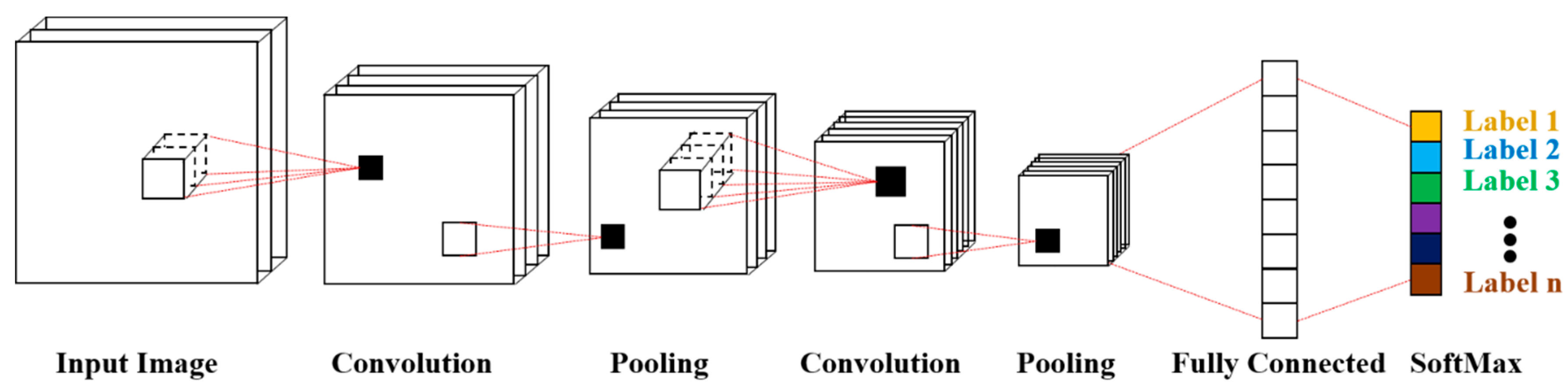
CNNs are a popular type of deep learning model consisting of convolutional layers, pooling layers, fully connected layers, and a softmax layer, as shown in Figure 2, which is described in Section 3. CNNs are appropriate for large-scale image processing because of the sparse interactions and weight sharing resulting from the convolution computation. In CNNs, the sparse interaction means that the units in a higher layer are connected with units with a limited scale, i.e., the receptive field in the lower layer. Weight sharing means that the units in the same layer share the same connection weights, i.e., the convolution filters, decreasing the number of parameters in the CNN. The convolution computation makes it possible for the response of the units of the deepest layer of the network to be dependent only upon the shape of the stimulus pattern, and they are not affected by the position where the pattern is presented. Given a convolutional layer, its output can be obtained as follows:
where denotes the output of layer , is the input of layer , and is the convolution filters of layer .
In recent years, more complex structures and deeper networks have been developed. Lin et al. [44] proposed a “network in network” structure to enforce the abstract ability of the convolutional layer. Based on the method proposed by Lin et al. [44], Szegedy et al. [43] designed a more complex network structure by applying an inception module. In AlexNet [45], there are eight layers, in addition to the pooling and contrast normalization layers; however, in VGGNet and GoogLeNet, the depths are 19 and 22, respectively. More recently, much deeper networks have been proposed [46,47].
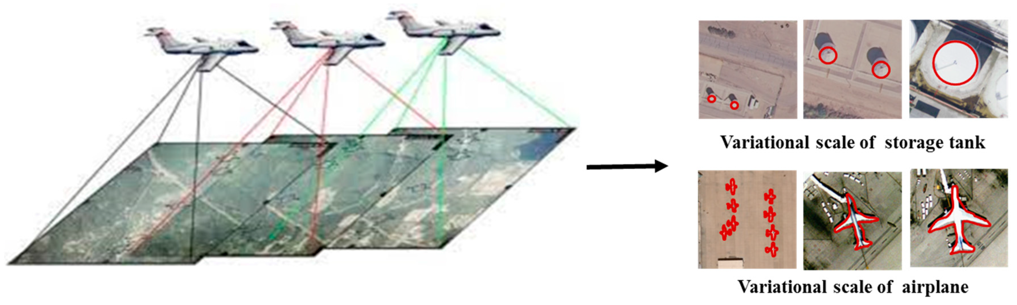
Due to the excellent performance of CNNs in image classification, a number of methods based on CNNs for remote sensing scene classification have been proposed, significantly improving classification accuracy. However, these methods do not consider the object scale variation problem in the remote sensing data, which means that the extracted features lack robustness to the object scale change, leading to misclassification of the scene image. The objects contained in the scene image play an important role in scene classification [48,49]. However, the same objects in remote sensing images can have different scales, as shown in Figure 3, resulting in them being difficult to capture. It is easy to classify a scene image containing objects with a common scale; however, those images containing objects with a changed scale can easily be wrongly classified. Taking the two images of storage tanks and airplanes in Figure 3 as examples, the right images are easy to classify, but it is almost impossible to recognize the left images as storage tanks/airplanes because of the different scales of the images.
3. Scene Classification for HSR Imagery Based on a Deep Random-Scale Stretched Convolutional Neural Network
To solve this object scale problem, the main idea in this paper is to generate multiple-scale samples to train the CNN model, forcing the trained CNN model to correctly classify the same image with different scales. To help make things easier, the scale variation is modeled as follows in this paper:
where is the true scale; denotes the scale variation factor, obeying a normal or uniform distribution, i.e., or ; and represents the changed scale. Once and are known, can be obtained by , and given an image I with scale , image is obtained by stretching into and then feeding it into the CNN to extract the features. According to this assumption, the goal of making the features extracted by the CNN robust to scale has been transformed into making the features robust to , i.e., the trained CNN can correctly recognize image with various values of . To achieve this, for each image, multiple samples are sampled, and multiple corresponding stretched images are obtained to force the CNN to be robust to α in the training phase. Meanwhile, in the CNN, in order to increase the number of image samples, the patches cropped from the image are fed into the CNN, instead of the whole image. Assuming that the scale of the patches is , the patches should be cropped from the stretched image with scale . Finally, there are three steps to generating the patches that are fed into the CNN, as follows:
(1) Sample from or ;
(2) Stretch an image of to , where ;
(3) Crop a patch with scale from the stretched image obtained in step 2.
However, in practice, due to the linearity of Equation (2), the above steps can be translated into the following steps to save memory:
(1) Sample from or ;
(2) Compute the cropping scale and crop a patch with scale from image . In this step, the upper-left corner of the cropped patch in image is determined by randomly selecting an element from where is the samples and lines of the whole image .
(3) Stretch the cropped patch obtained in step 2 into .
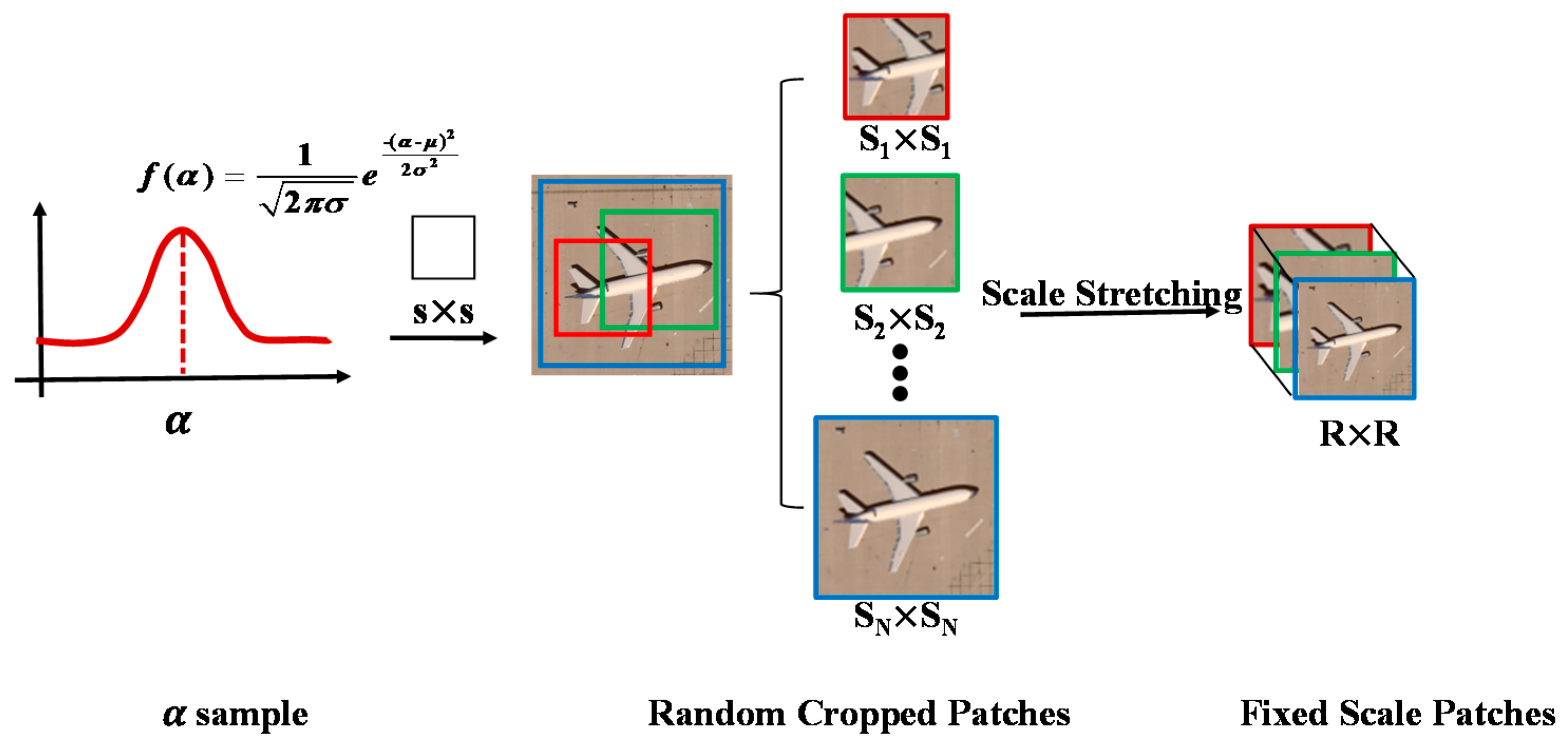
For every image in the dataset, we repeat the above three steps and finally obtain multiple-scale samples from the images, as shown in Figure 4. In this paper, the two kinds of distribution for α are respectively tested, and the results are discussed in Section 5. The parameter is set to 1.2 by experience, and bilinear interpolation is adopted in the random-scale stretching as a trade-off between computational efficiency and classification accuracy. In the proposed method, there will be many patches cropped from every image. However, the number of patches is not determined explicitly. Instead, we determine the number of patches by determining the number of training iterations. Assuming that the number of training samples is m, for training, the number of iterations is set as N, where N is 70 K in this paper, and for each iteration, there are n patches cropped from the n (set as 60 in this paper) images and fed into the CNN model. Therefore, for the training, the number of patches required is N × n, which means that the number of patches from every training image is . In testing, the cropped patch number is set by experience.
On the one hand, this can be regarded as a data augmentation strategy for remote sensing image scene classification, which could be combined with other data augmentation methods such as occlusion, rotation, mirroring, etc. On the other hand, the random-scale stretching is a process which adds structure noise to the input. Differing from the denoising auto-encoders, which add value noise to the input to force the model to learn robust features, SRSCNN focuses on structure noise, i.e., the scale change of the objects. Similar to the denoising auto-encoders, the input of the model is corrupted with random noise following a definite statistical distribution, i.e., a uniform or normal distribution.
3.1. SRSCNN
The proposed SRSCNN method integrates random-scale stretching and a CNN, and can be divided into three parts: (1) data pre-processing; (2) random-scale stretching; and (3) CNN model training. In this paper, the image is represented as a tensor with dimensions of H × W × 3, where H and W represent the height and width of the image, respectively.
Data pre-processing: To accelerate the learning convergence of the CNN, normalization is required. This is usually followed by the z-score to centralize the data distribution. However, to keep things simple, in this paper, pixels are normalized to [0, 1] by dividing them by the maximum pixel value:
where is the normalized image, and is the maximum pixel value in the image.
Random-scale stretching: In the proposed method, random-scale stretching is integrated with random rotation, which are common data augmentation methods in CNN training. Given a normalized image , the image output of the random-scale stretching is obtained as follows:
where stands for the random-scale stretching, and denotes the random rotation of degrees, where is 0, 90, 180, or 270.
CNN model training: After the random-scale stretching, the image is fed into the CNN model, which consists of convolutional layers, pooling layers, a fully connected layer, and a softmax layer.
Convolutional layers: Differing from the traditional features utilized in scene classification, where spectral features such as the spectral mean and standard deviation, and spatial features such as SIFT, are selected and extracted artificially, the convolutional layers can automatically extract features from the data. There are multiple convolution filters in each layer, and every convolution filter corresponds to a feature detector. For convolutional layer t (t ≥ 1), given the input , the output of convolutional layer t can be obtained by Equations (6) and (7):
where represents the kth convolutional filter corresponding to the ith output feature map, denotes the kth feature map of , is the bias corresponding to the ith output feature map, is the convolution computation, and f is the activation function, is ith output feature map of . As Equation (6) shows, the convolution is a linear mapping, and is always followed by a non-linear activation function f such as sigmoid, tanh, SoftPlus, ReLU, etc. In this paper, ReLU is adopted as the activation f due to its superiority in convergence and its sparsity compared with the other activation functions [50,51,52]. ReLU is a piecewise function:
Pooling layers: Following the convolutional layers, the pooling layers expect to achieve a more compact representation by aggregating the local features, which is an approach that is more robust to noise and clutter and invariant to image transformation [53]. The popular pooling methods include average pooling and max pooling. Max pooling is adopted in this paper:
where is the scale of the pooling kernel.
Fully connected layer: The fully connected layer can be viewed as a special convolutional layer whose output height and width are 1, i.e., the output is a vector. In addition, in this paper, the fully connected layer is followed by dropout [54], which is a regularizer to prevent co-adaptation since a unit cannot rely on the presence of other particular units because of the random presence of them in the training phase.
Softmax layer: In this paper, softmax is added to classify the features extracted by the CNN. As a generalization of logistic regression for a multi-class problem, softmax outputs a vector whose every element represents the possibility of a sample belonging to each class, as shown in Equation (10):
where represents the possibility of sample i’s label being t. Based on maximum-likelihood theory, loss function of softmax can be obtained as follows:
where is the number of samples, and the second term is the regularization term, which is always the L2-norm, to avoid overfitting. is the coefficient to balance these two terms. The chain rule is applied in the back-propagation for computing the gradient to update the parameters, i.e., the weight and bias in CNN. Take the layer t as an example. To determine the values of and bias in layer t, the stochastic gradient descent method is performed:
(1) Compute the objective loss function in Equation (11);
(2) Based on the chain rule, compute the partial derivative of and bias :
(3) Update the values of and bias :
where is the learning rate. In the training phase, the above three steps are repeated until the required number of iterations (set as 70 K in this paper) is reached. The procedure of SRSCNN is presented in Algorithm 1, where random rotation is integrated with random-scale stretching.
| Algorithm 1. The SRSCNN procedure |
| Input: |
| -input dataset D = {(I, y) | I∈RH×W×3, y∈{1, 2, 3, …C} |
| -scale of patch R |
| -batch size m |
| -scale variation factor obeying distribution d |
| -defined CNN structure Net |
| -maximum iteration times L |
| Output: |
| -Trained CNN model |
| Algorithm: |
| 1. randomly initialize Net |
| 2. for l = 1 to L do |
| 3. generate a small dataset P with |P| = m from D |
| 4. for I = 1 to m do |
| 5. normalize IiP to [0, 1] by dividing by the maximum pixel value to obtain the normalized image Iin. |
| 6. generate a random-scale stretched patch pi from Iin. |
| 7. P = P − {Ii}, P = P∪{pi} |
| 8. end for |
| 9. Feed P to Net, update parameters W and b in Net |
| 10. end for |
According to recent deep learning theory [42,43], representation depth is beneficial for classification accuracy. However, the structure like GoogLeNet and VGGNet cannot be directly used because of the small size of remote sensing datasets compared with the ImageNet dataset with millions of images. Therefore, in this paper, a network structure similar to VGGNet is adopted, making a trade-off between the depth and the number of images in the dataset, where every two convolutional layers are stacked. The main structure configuration adopted in this paper is shown in Table 1. In Table 1, the convolutional layer is denoted as “ConvN–K”, where N denotes the convolutional kernel size and K denotes the number of convolutional kernels. The fully connected layer is denoted as “FC–L”, where L denotes the number of units in the fully connected layer. The effect of L on the scene classification accuracy is analyzed in Section 5.
3.2. Remote Sensing Scene Classification
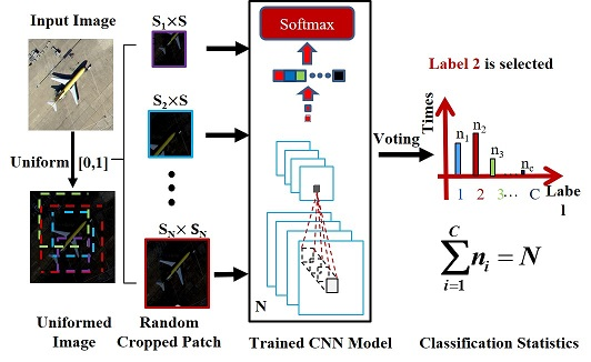
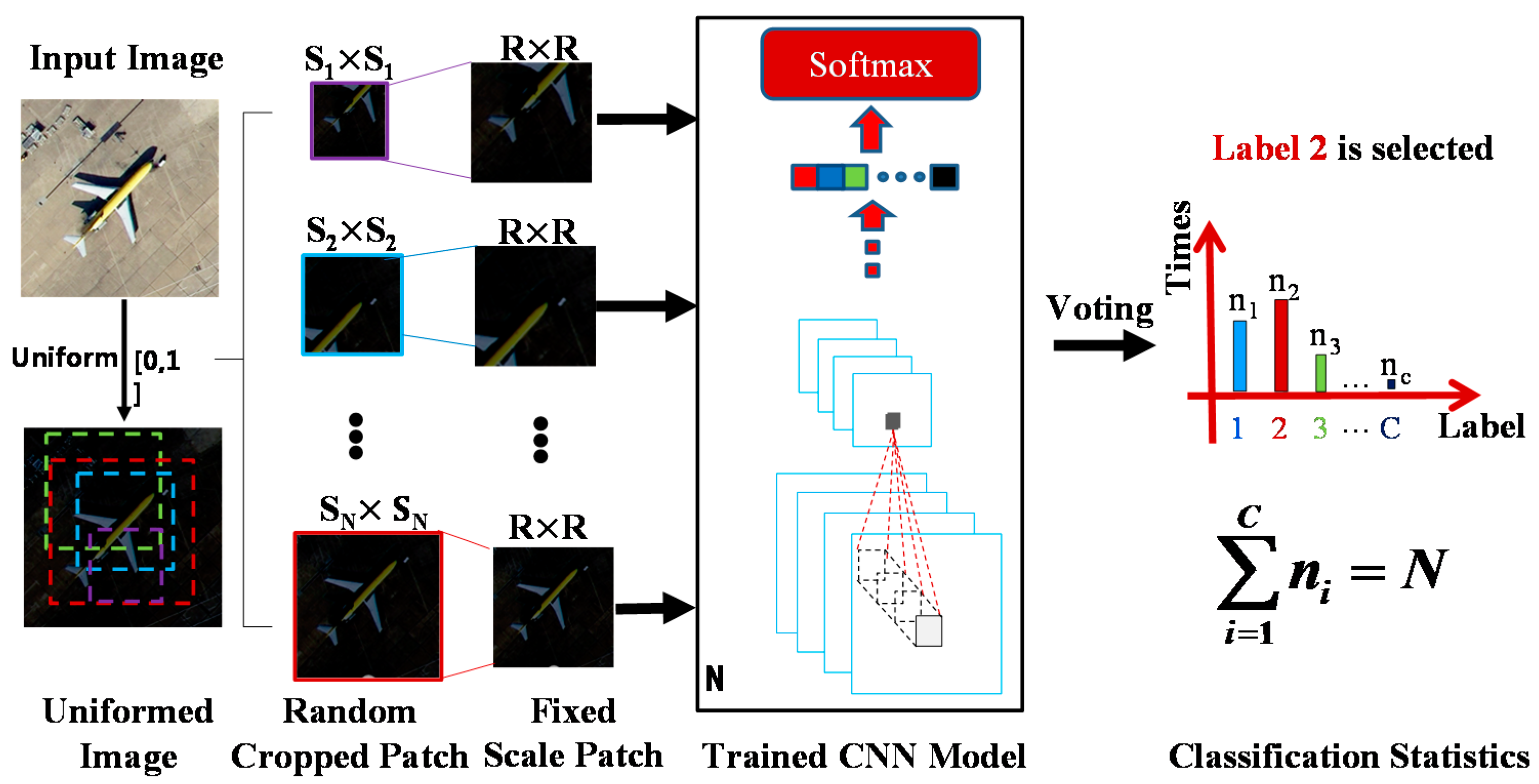
In the proposed method, the different patches from the same image contain different information, so every feature extracted from a patch can be viewed as a perspective of the scene label of the image where the patch is cropped from. To further improve the scene classification performance, a robust scene classification strategy is adopted, i.e., multi-perspective fusion. SRSCNN randomly crops a patch with a random scale from the image and predicts its label using the trained CNN model, under the assumption that the patch’s label is identical to the image’s label. For simplicity, in this paper, the perspectives have identical weights, and voting is finally adopted, which means that SRSCNN classifies a sample multiple times and decides its label by selecting the class for which it is classified the most times. In Figure 5, multiple patches with different scales and different locations are cropped from the image, and these patches are then stretched to a specific scale as the input of the trained model to predict its label. Finally, the labels belonging to these patches are counted and the label occurring the most times is selected as the label of the whole image (Class 2 is selected in the example in Figure 5). To demonstrate the effectiveness of the multi-perspective fusion, three tests were performed on three datasets, which are described in Section 4.
4. Experiments and Results
The UCM dataset, the Google dataset of SIRI-WHU, and the Wuhan IKONOS dataset were used to test the proposed method. The traditional methods of BoVW, LDA, the spatial pyramid co-occurrence kernel++ (SPCK++) [2], the efficient spectral-structural bag-of-features scene classifier (SSBFC) [7], locality-constrained linear coding (LLC) [7], SPM+SIFT [7], SAL-PTM [10], the Dirichlet-derived multiple topic model (DMTM) [14], , SIFT+SC [55], the local Fisher kernel-linear (LFK-Linear), the Fisher kernel-linear (FK-Linear), the Fisher kernel incorporating spatial information (FK-S) [56], and methods based on deep learning, i.e., saliency-guided unsupervised feature learning (S-UFL) [37], the gradient boosting random convolutional network (GBRCN) [40], the large patch convolutional neural network (LPCNN) [41], and the multiview deep convolutional neural network (M-DCNN) [36], were compared. In the experiments, 80% of the samples were randomly selected from the dataset as the training samples, and the rest were used as the test samples. The experiments were performed on a personal computer equipped with dual Intel Xeon E5-2650 v2 processors, a single Tesla K20m GPU, and 64 GB of RAM, running Centos 6.6 with the CUDA 6.5 release. For each experiment, the training was stopped after 70 K iterations, taking about 2.5 h. Each experiment on each dataset was repeated five times, and the average classification accuracy was recorded. To keep things simple, CCNN denotes the common CNN without random-scale stretching and multi-perspective fusion, CNNV denotes the common CNN with multi-perspective fusion but not random-scale stretching, SRSCNN-NV denotes the CNN with random-scale stretching but not multi-perspective fusion.
4.1. Experiment 1: The UCM Dataset
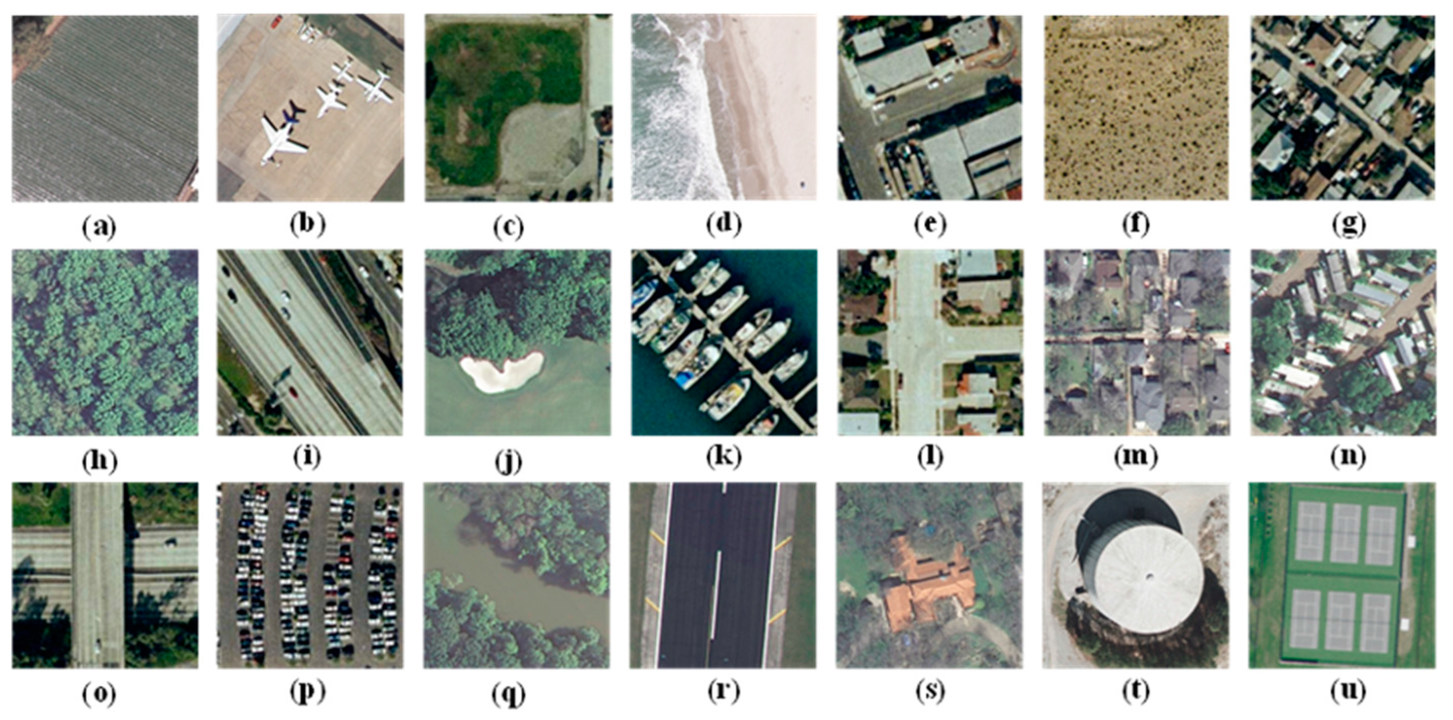
To demonstrate the effectiveness of the proposed SRSCNN, the 21-class UCM land-use dataset collected from large optical images of the U.S. Geological Survey was used. The UCM dataset covers various regions of the United States, and includes 21 scene categories, with 100 scene images per category. Each scene image consists of 256 × 256 pixels, with a spatial resolution of one foot per pixel. Figure 6 shows representative images of each class, i.e., agriculture, airplane, baseball diamond, beach, buildings, chaparral, dense residential, forest, freeway, golf course, harbor, intersection, medium residential, mobile home park, overpass, parking lot, river, runway, sparse residential, storage tanks, and tennis court.
From Table 2, it can be seen that SRSCNN performs well and achieves the best classification accuracy. The main reason for the comparatively high accuracy achieved by SRSCNN when compared with the non-deep learning methods such as BoVW, LDA, and LLC is that SRSCNN, as a deep learning method, can extract the essential features from the data directly, without prior information, and is a joint learning method which combines feature extraction and scene classification into a whole, leading to the interaction between feature extraction and scene classification during the training phase. Compared with the methods based on deep learning, i.e., S-UFL, GBRCN, LPCNN, and M-DCNN, SRSCNN again achieves a comparatively high classification accuracy. The reason SRSCNN achieves a better accuracy is that the objects in scene classification make a big difference; however, the previous methods based on deep learning do not consider the scale variation of the objects, resulting in a challenge for the scene classification. In contrast, in order to solve this problem, random-scale stretching is adopted in SRSCNN during the training phase to ensure that the extracted features are robust to scale variation. In order to further demonstrate the effectiveness of the random-scale stretching, two experiments were conducted based on CCNN and SRSCNN-NV, respectively. From Table 2, it can be seen that SRSCNN-NV outperforms CCNN by 1.02%, which demonstrates the effectiveness of the random-scale stretching for remote sensing images. Meanwhile, compared with SRSCNN-NV, SRSCNN is 2.99% better, which shows the power of the multi-perspective fusion. According to the above comparison and analysis, it can be seen that the random-scale stretching and multi-perspective fusion enable SRSCNN to obtain the best results in remote sensing image scene classification. The Kappa of SRSCNN for the UCM is 0.95.
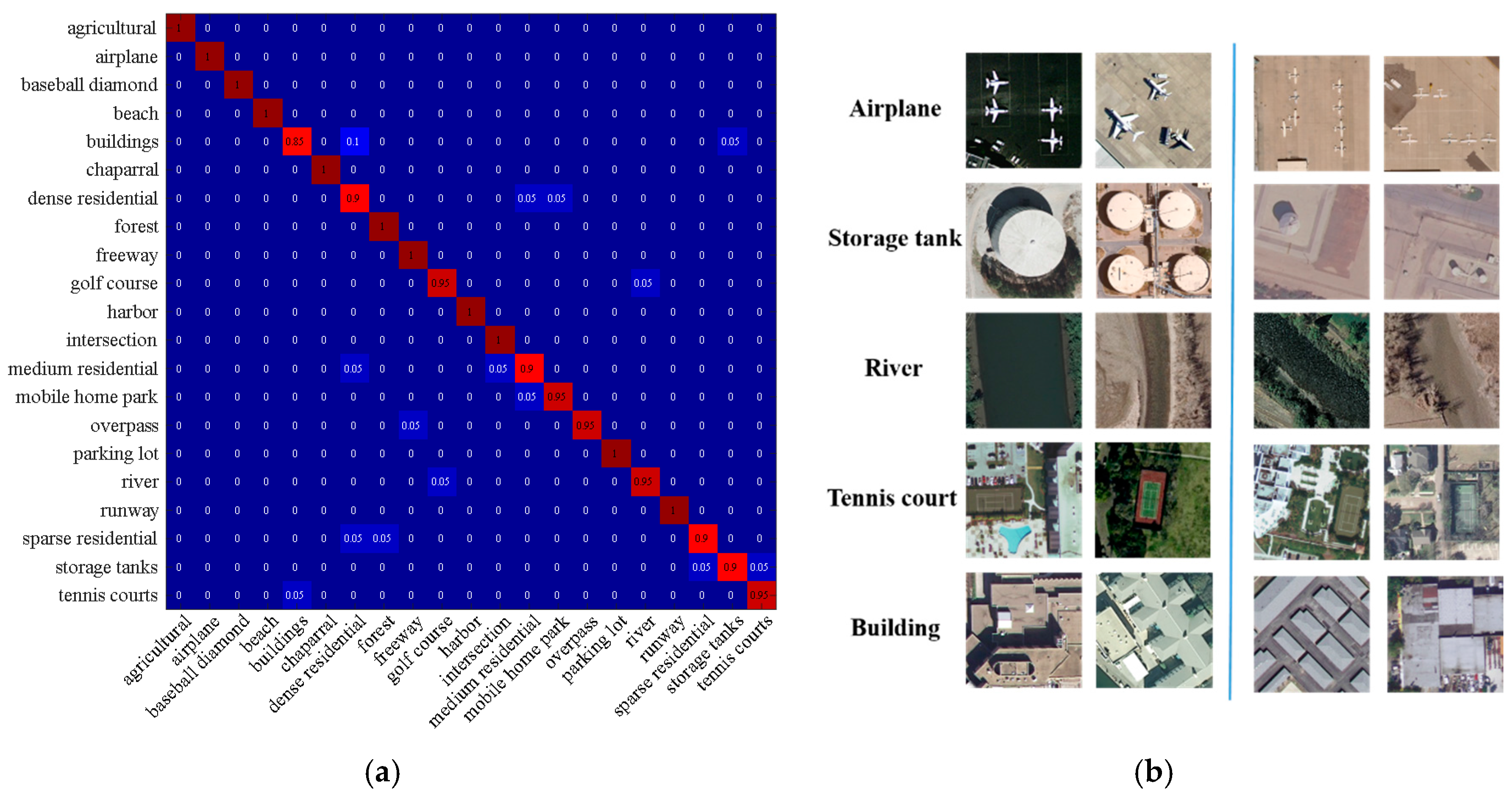
From Figure 7a, it can be seen that the 21 classes can be recognized with an accuracy of at least 85%, and most categories are recognized with an accuracy of 100%, i.e., agriculture, airplane, baseball diamond, beach, etc. From Figure 7b, it can be seen that some representative scene images on the left are recognized correctly by SRSCNN and CNNV. It can also be seen that when the scale of the objects varies, CNNV cannot correctly recognize them, but SRSCNN does, due to its ability to extract features that are robust to scale variation. Taking the airplane scenes as an example, the two images on the left are easy to classify, because the scales of the airplanes in these images are normal; however, the airplanes in the right images are very difficult to recognize, because of their different scale, leading to misclassification by CNNV. However, the proposed SRSCNN can still recognize them correctly due to its ability to extract features that are robust to scale change.
4.2. The Google Dataset of SIRI-WHU
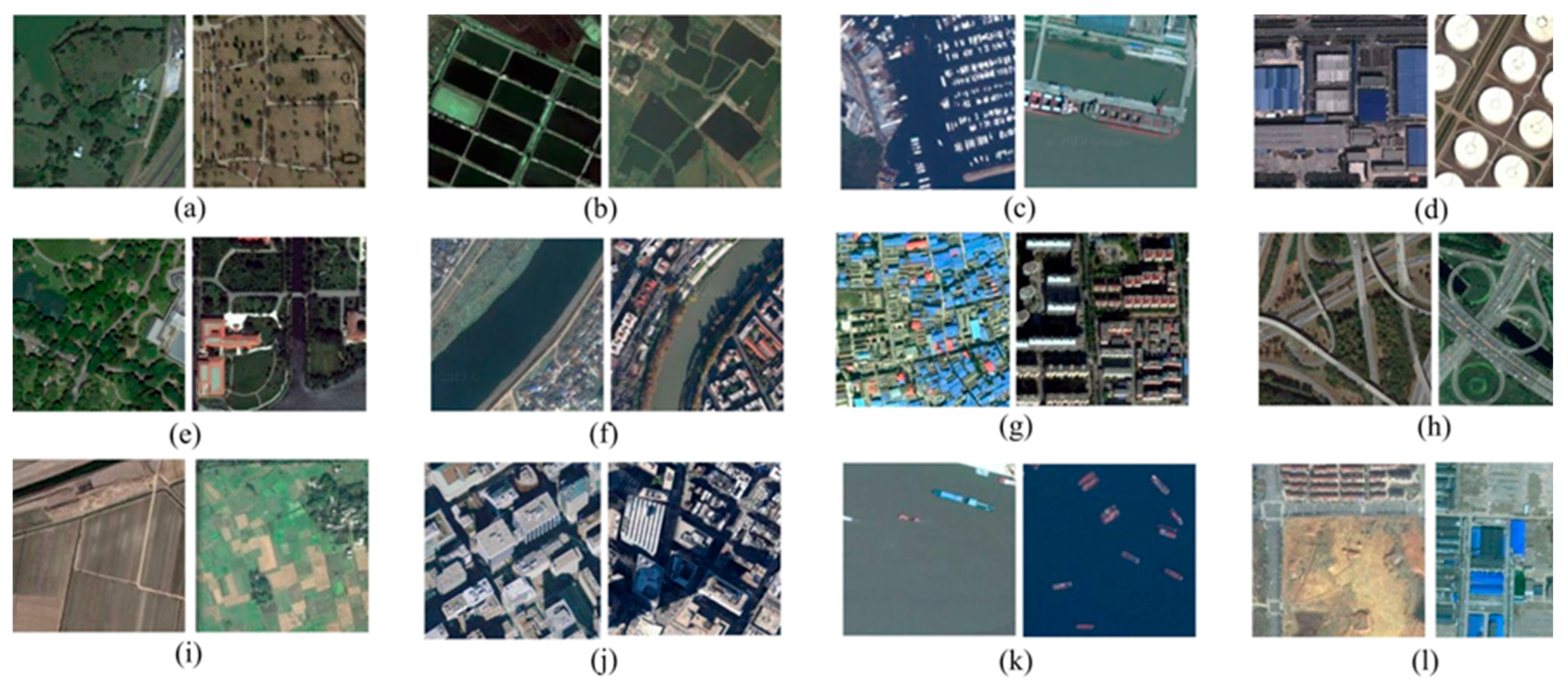
The Google dataset of SIRI-WHU designed by the Intelligent Data Extraction and Analysis of Remote Sensing (RSIDEA) Group of Wuhan University contains 12 scene classes, with 200 scene images per category, and each scene image consists of 200 × 200 pixels, with a spatial resolution of 2 m per pixel. Figure 8 shows representative images of each class, i.e., meadow, pond, harbor, industrial, park, river, residential, overpass, agriculture, commercial, water, and idle land.
From Table 3, it can be seen that SRSCNN performs well and achieves the best classification accuracy. The main reason for the comparatively high accuracy achieved by SRSCNN when compared with the traditional scene classification methods such as BoVW, LDA, and LLC is that SRSCNN, as a deep learning method, can extract the essential features from the data directly, without prior information, and combines feature extraction and scene classification into a whole, leading to the interaction between feature learning and scene classification. Compared with the deep learning methods, S-UFL and LPCNN, SRSCNN performs 19.92% and 4.88% better, respectively. The reason SRSCNN achieves a better accuracy is that S-UFL and LPCNN do not consider the scale variation of objects, resulting in a challenge for the scene classification. In contrast, in order to meet this challenge, random-scale stretching is adopted in SRSCNN during the training phase to ensure that the extracted features are robust to scale variation. Compared with SSBFC, DMTM, and FK-S, with only 50% of the samples randomly selected from the dataset as the training samples, the proposed method still performs the best, which is shown in Table 4. In order to further demonstrate the effectiveness of the random-scale stretching, two experiments were conducted based on CCNN and SRSCNN-NV, respectively. From Table 3, it can be seen that SRSCNN-NV outperforms CCNN by 2.80%, demonstrating the effectiveness of the random-scale stretching for remote sensing images. Meanwhile, compared with SRSCNN-NV, SRSCNN is 3.70% better, showing the power of the multi-perspective fusion. According to the above comparison and analysis, it can be seen that the random-scale stretching and multi-perspective fusion enable SRSCNN to obtain the best results in remote sensing image scene classification. The Kappa of SRSCNN for the Google dataset of SIRI-WHU is 0.9364 when 80% training samples selected.
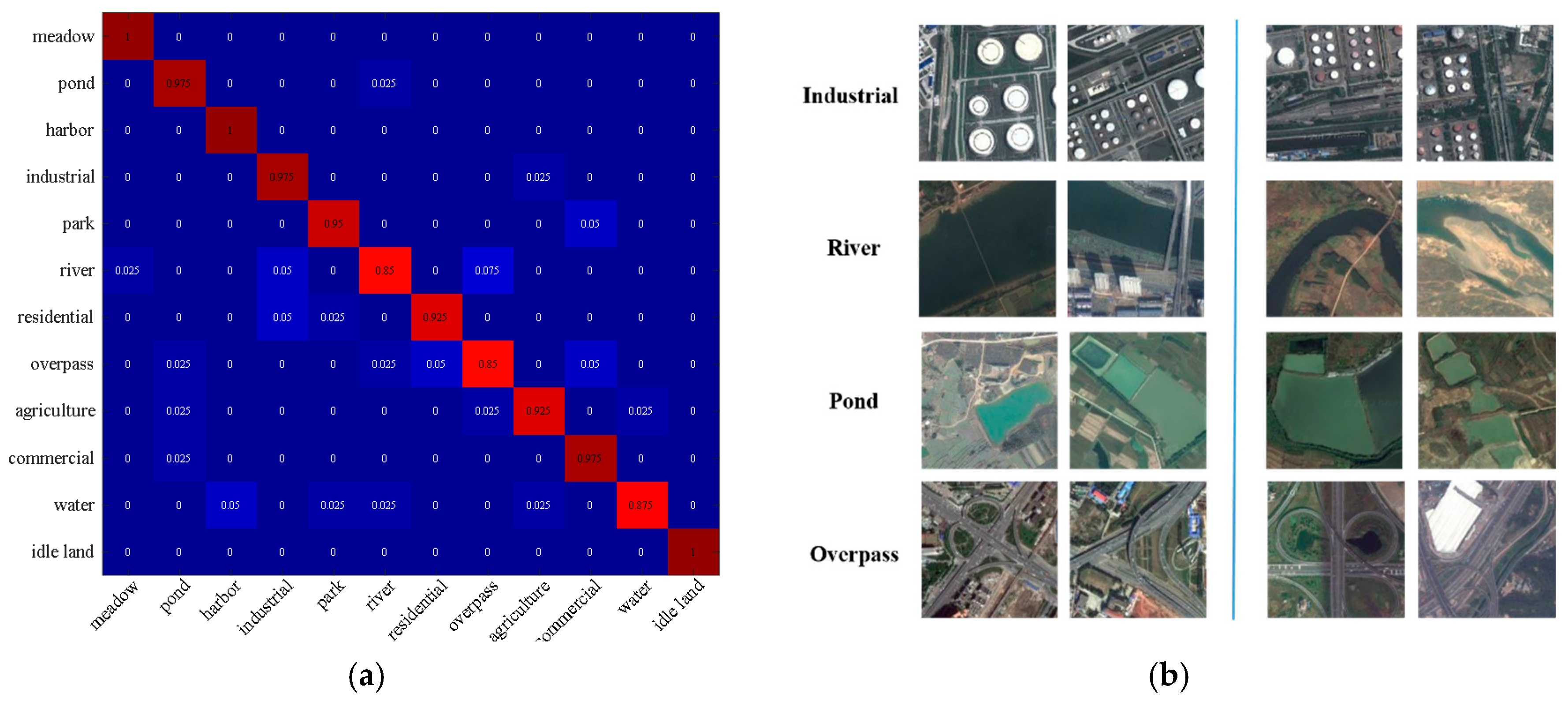
From Figure 9a, it can be seen that most of the classes can be recognized with an accuracy of at least 92.5%, except for river, overpass, and water. Meadow, harbor, and idle land are recognized with an accuracy of 100%. From Figure 9b, it can be seen that some representative scene images on the left are recognized correctly by SRSCNN and CNNV, i.e., CNN with voting but not random-scale stretching. It can also be seen that when the object scale varies, CNNV cannot correctly recognize the objects, but SRSCNN correctly recognizes them due to its ability to extract features that are robust to scale variation.
4.3. Experiment 3: The Wuhan IKONOS Dataset
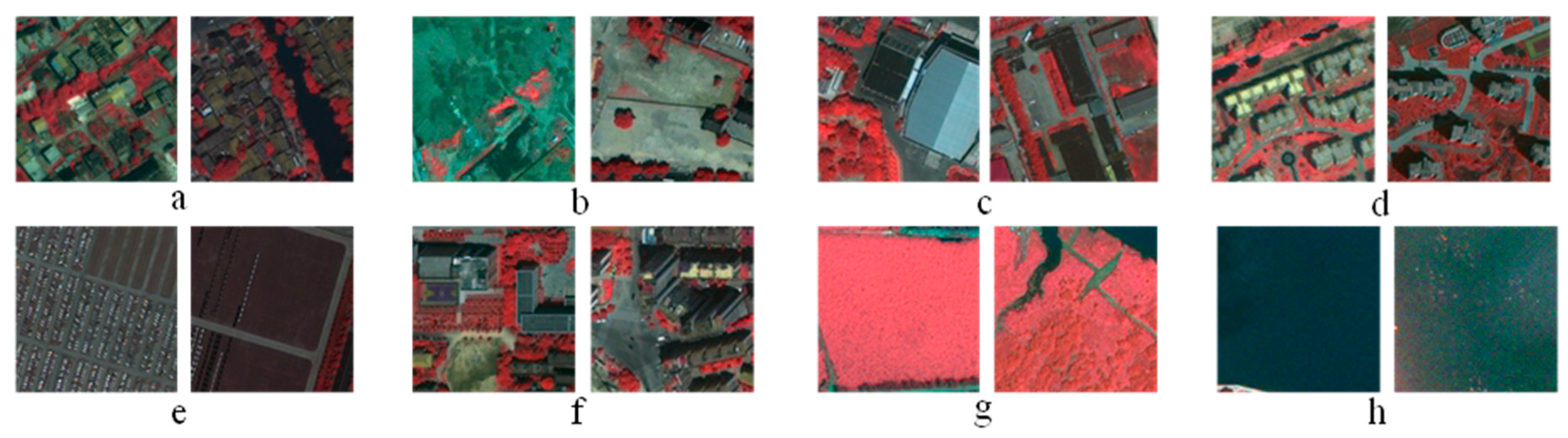
The HSR images in the Wuhan IKONOS dataset were acquired over the city of Wuhan in China by the IKONOS sensor in June 2009. The spatial resolutions of the panchromatic images and the multispectral images are 1 m and 4 m, respectively. In this paper, all the images in the Wuhan IKONOS dataset were obtained by Gram–Schmidt pan-sharpening with ENVI 4.7 software. The Wuhan IKONOS dataset contains eight scene classes, with 30 scene images per category, and each scene image consists of 150 × 150 pixels, with a spatial resolution of 1 m per pixel. These images were cropped from a large image obtained over the city of Wuhan in China by the IKONOS sensor in June 2009, with a size of 6150 × 8250 pixels. Figure 10 shows representative images of each class, i.e., dense residential, idle, industrial, medium residential, parking lot, commercial, vegetation, and water.
From Table 5, it can be seen that SRSCNN performs well and achieves a better classification accuracy than BoVW, LDA, P-LDA, FK-Linear, and LFK-Linear. However, compared with BoVW and P-LDA, the methods based on CNN such as CCNN and SRSCNN-NV perform worse, and accuracy improvement is limited in SRSCNN. The reason is that the large dataset is usually required to train the CNN model, but there are only about 200 images for training. In Table 5, there is no big difference in accuracy between CCNN and SRSCNN-NV. The main reason for this is that this dataset is cropped from the same image, and the effect of the scale change problem is small. However, compared with SRSCNN-NV, SRSCNN performs 10.03% better, and still performs the best. The Kappa of SRSCNN for the Wuhan IKONOS dataset is 0.8333.
An annotation experiment on the large IKONOS image was conducted with the trained model. During the annotation of the large image, the large image was split into a set of scene images where the image size and spacing are set to pixel and pixels, respectively. The set of scene images is denoted as . Then the images in were classified by the trained model. Finally, the annotation result can be obtained by assembling the images in . In addition, for the overlapping pixels between adjacent images, their class labels were determined by the majority voting rule. The annotation result is shown in Figure 11.
5. Discussion
To avoid overfitting, dropout technology is applied in the proposed method. Four different dropout rates were tested to analyze how this affects classification accuracy. After feature extraction, the number of units in the last fully connected layer decides the length of the feature, which plays an important role in the classification results. In Section 4, we analyzed the classification results when the length of the feature (i.e., the number of units in the fully connected layer of the adopted CNN model in Table 1) was equal to 600. In this section, the sensitivity analysis between length of feature and classification accuracy is described. In SRSCNN, we add random-scale stretching to the CNN to improve the remote sensing image scene classification. To investigate the effect of the distribution of the scale variation factor α, a sensitivity analysis of different distributions is undertaken. In addition, for a scene image with a fixed scale, the crop rate decides the approximate crop scale, so three different crop rates are analyzed. In SRSCNN, the random spatial scale stretching (Rss) and random rotation (Rot) are adopted, the analysis about effectiveness of random spatial scale stretching and random rotation is described. To test the influence of the spatial resolution, a sensitivity analysis of different resolution is undertaken. In training phase, the number of training samples cropped from each image is decided by the iteration times, so the different iterations are analyzed.
5.1. Sensitivity Analysis in Relation to the Dropout Rate
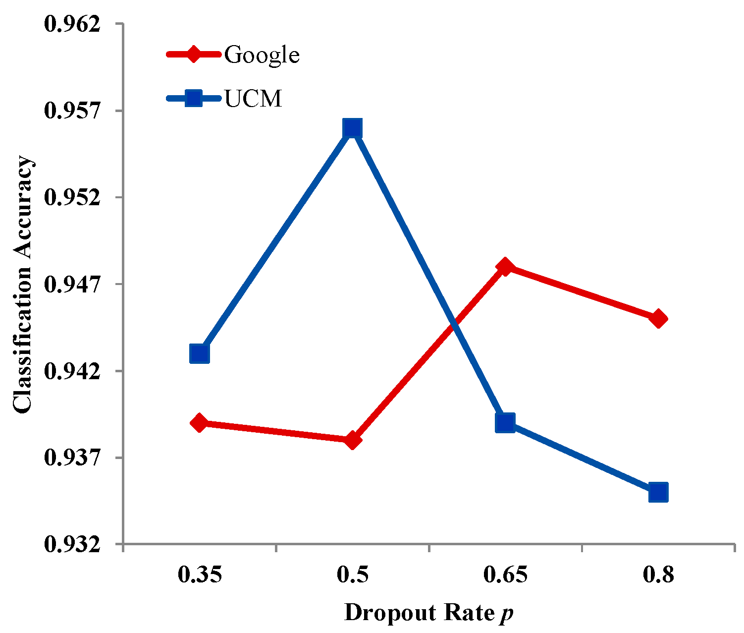
According to dropout theory, breaking the co-adaptation helps to make each hidden unit more robust, i.e., decreasing the reliance on other units and forcing the units to create useful features. Dropout is adopted in the proposed method, which involves the parameter dropout rate . In the training process, a unit is deleted with probability , and in order to make sure that the expectation of the hidden unit is unchanged, the output of the hidden unit is multiplied by () in the testing. To study the sensitivity of SRSCNN in relation to the dropout rate, experiments were undertaken with the UCM and Google datasets, respectively, and the other parameters were kept the same. From Figure 12, when the dropout rate increases from 0.35 to 0.5, classification accuracy of UCM improves; however, it begins to decrease when the dropout rate continues to increase, achieving the best classification result with a dropout rate of 0.5. For the Google dataset, although the change trend is not as obvious as for UCM, because of the slight decline at 0.5, it can be seen that when the dropout rate increases from 0.35 to 0.65, classification accuracy for the Google dataset improves, and it begins to decrease when the dropout rate continues to increase, achieving the best classification result with a dropout rate of 0.65.
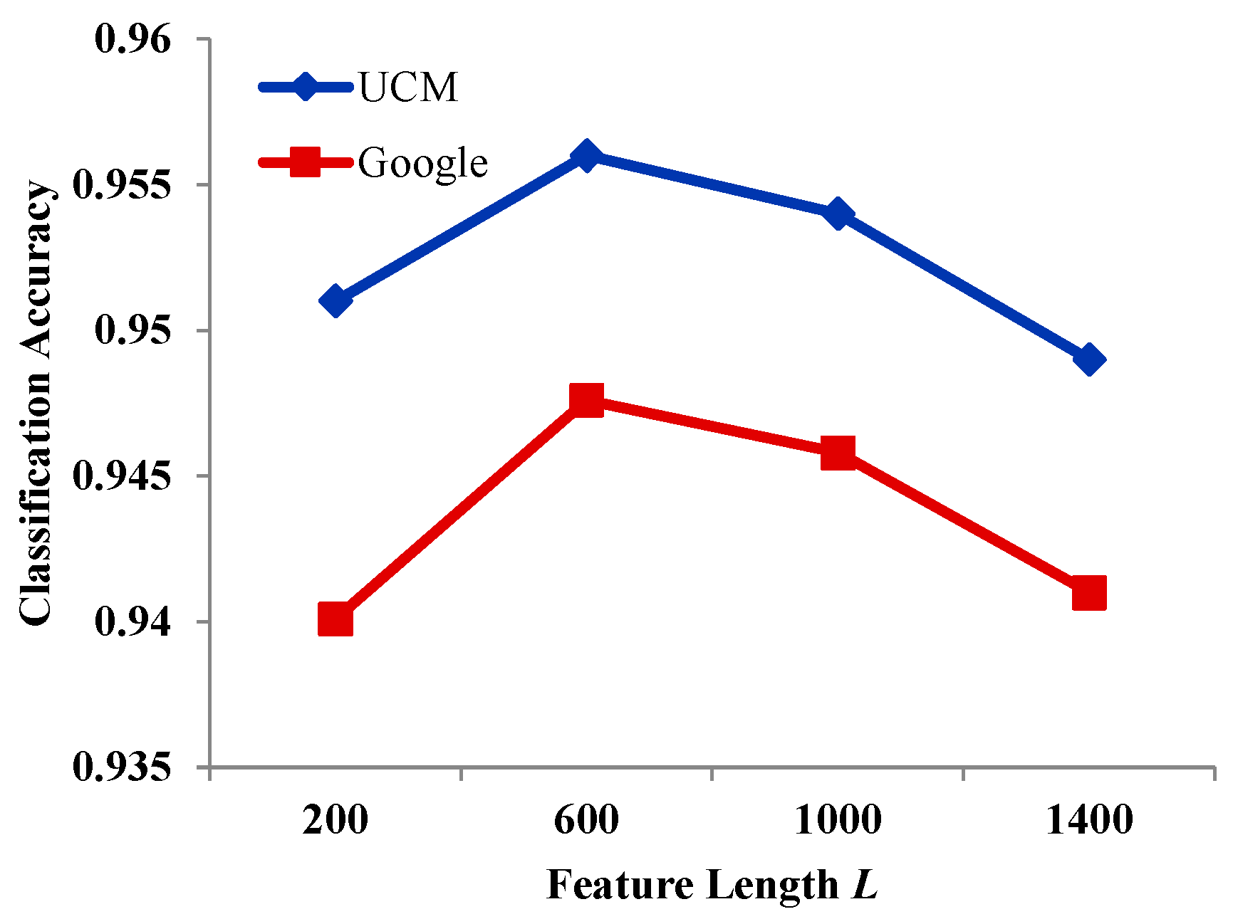
5.2. Sensitivity Analysis in Relation to the Length of the Feature
To investigate the effect of the length of the feature on classification accuracy, the other parameters were again kept the same. The value of the length of feature was varied as follows: = {200, 600, 1000, and 1400}. From Figure 13, as the length increases from 200 to 600, classification accuracy with the UCM dataset increases, and it then decreases when length > 600. However, accuracy at 1000 is still better than at 200. The reason for this may be that a feature with = 1000 has a more powerful representation ability with the 21-class UCM dataset. The optimal value of is around 600 for UCM. For the Google dataset, it has the same change trend as UCM, achieving the best accuracy at = 600.
5.3. Sensitivity Analysis in Relation to the Distribution of the Scale Variation Factor α
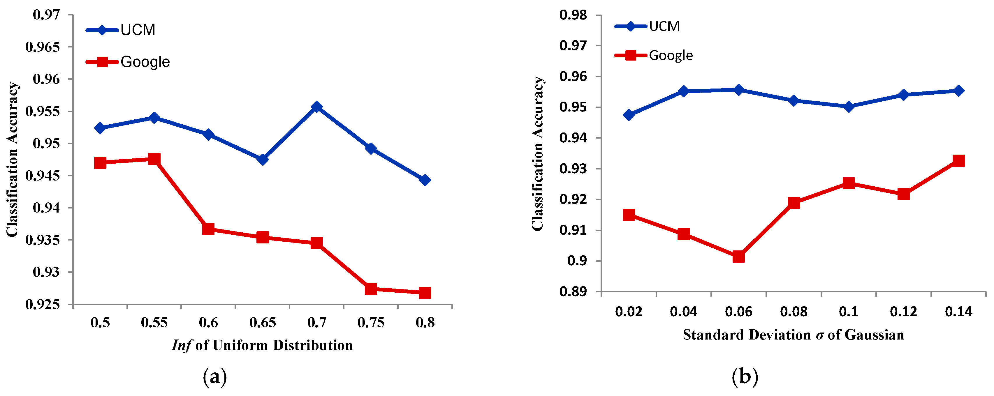
The distribution of α makes a great difference in HSR remote sensing image scene classification. When α obeys a normal distribution, i.e., , the standard deviation plays an important role in the classification results, and when α obeys a uniform distribution, i.e., , greatly affects classification accuracy. We tested the UCM and Google datasets with the two kinds of distribution, with the other parameters kept the same. From Figure 14a, in general, with the improvement of of the uniform distribution, classification accuracy with the UCM dataset decreases, but then leaps on some points, which is the same for the Google dataset. Both the UCM and Google datasets obtain their worst classification accuracy at 0.8. However, the UCM dataset obtains its best result at 0.7, and the Google dataset at 0.55. When satisfies a Gaussian distribution, the broad trend of remote sensing classification accuracy with the UCM dataset is slightly upwards in most places, although leaps do exist. Compared with the UCM dataset, classification accuracy with the Google dataset fluctuates significantly, but the trend is upwards in Figure 14b. In this paper, when , the smaller the value of , the bigger the stretch range. When , the bigger the value of , the bigger the stretch range. Therefore, from Figure 14, the conclusion can be made that a large stretch range helps to improve classification accuracy.
5.4. Sensitivity Analysis in Relation to the Crop Rate Cr
In this paper, the ratio between the specified scale and the original image scale is defined as the crop rate , i.e., , where S is 256 for the UCM dataset and 200 for the Google dataset. Different crop rates lead to different basic scales of patches cropped from an image, and patches with different scales may contain different information. We therefore analyzed how the crop rate affects classification accuracy, and the results are shown in Table 6. The other parameters were again kept the same. For the UCM and Google datasets, when ranges between 50–70%, classification accuracy fluctuates within a narrow range and get the optimal or suboptimal result. In addition, when reaches around 90%, it begins to rapidly fall.
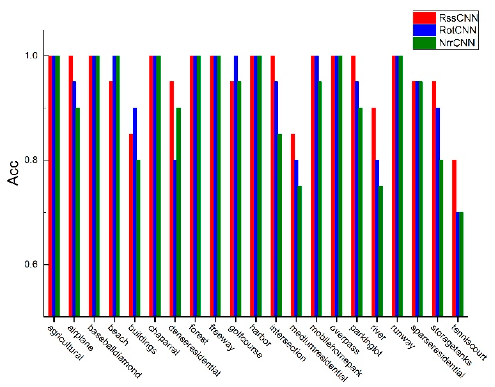
5.5. Sensitivity Analysis in Relation to the Rss and Rot
In this paper, the random spatial scale stretching (Rss) and random rotation (Rot) are adopted, and we analyzed how the Rss and Rot affect classification accuracy. First, the CNN with only with random spatial scale stretching or random rotation were denoted as RssCNN and RotCNN respectively and the CNN without random spatial scale stretching and random rotation was denoted as NrrCNN. The result is shown in Figure 15. From Figure 15, it can be seen that there is no difference between the RSSCNN, RotCNN and NrrCNN for some scene classes such as agricultural, chaparral and overpass, which means that these scene classes are largely unaffected by the random spatial scale stretching and random rotation. However, for the scene classes such as airplane and storage tank, the spatial scale stretching and random rotation had a relatively large impact. The main reason is that the scene classes such as airplane, storage tank, are object-centered, i.e., the scene class of an image is decided by the object it contains and the random spatial scale stretching or random rotation can help make the CNN to capture the objects for the object-centered scene.
5.6. Sensitivity Analysis in Relation to the Spatial Resolution
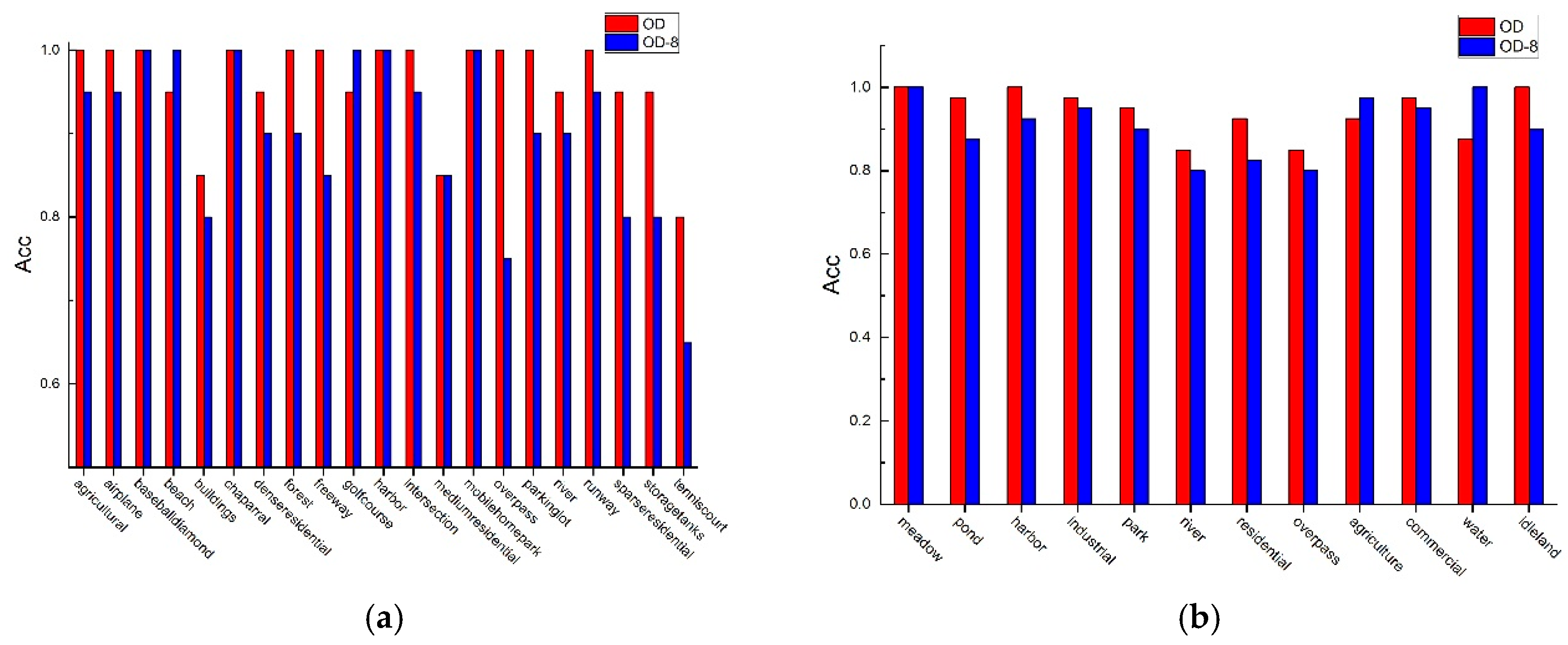
To test the effectives of the proposed method, three datasets with different spatial resolution, i.e., the UCM with spatial resolution 0.3 m, the Google dataset of SIRI-WHU with 2 m and the Wuhan IKONOS with 1m, are tested. From the experiment in Section 4, it can be seen that the proposed method can work well on these three different spatial resolution images. In addition, to test the influence of the spatial resolution in accuracy, four lower spatial resolution datasets are derived from the UCM and the Google dataset of SIRI-WHU by factor of 4 and 8 down-sampling. We denote the original data as OD, and the data obtained by factor of 4 and 8 down-sampling are denoted as OD-4 and OD-8. The accuracy comparison is shown in Table 7.
From the Table 7, it can be seen that accuracy fell when the spatial resolution decreases and accuracy falls rapidly with factor 8 down-sampling. To explore how the scene classes are affected by the spatial resolution, we compare the class accuracy of OD and OD-8 in Figure 16. From Figure 16, it can be seen that the accuracy of most scene classes falls when the spatial resolution decreased, particularly for the object-center scene classes such as airplane, storage tank. The main reason is that when the resolution decreases, it will be difficult to capture the key objects such as airplane, storage tank for the object-center scene.
5.7. Sensitivity Analysis in Relation to the Training Iteration
In SRSCNN, the training samples are cropped from each image and the training samples within each image may be different. Given the total training sample number n, the batch size m, the number of training samples extracted from each image is determined by:
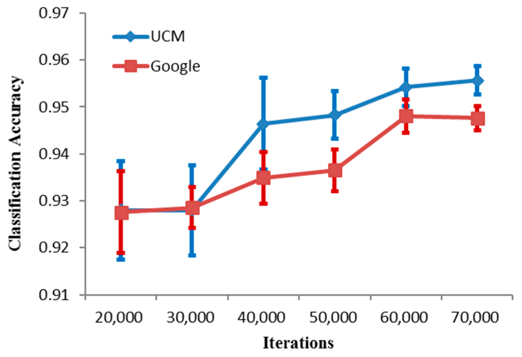
where denotes the number of training samples extracted from each image. From Equation (16), it can be seen that the is proportional to the iteration N. To explore how the number of iteration affects accuracy, the accuracy comparison between different training iteration times is shown in Figure 17. From Figure 17, it can be seen that accuracy increases with iteration times before 60000 and the standard deviation falls as the iteration times get larger. When the iteration times is equal to 70,000, there will be about 2200 training sample extracted from each image for training, and it can get the optimal or suboptimal result and the standard deviation become smaller. The main reason the standard deviation falls as the iteration times get larger is the will become larger, which means there will be more training samples extracted from each image.
6. Conclusions
In this paper, SRSCNN, a novel algorithm based on a deep convolutional neural network, has been proposed and implemented to solve the object scale change problem in remote sensing scene classification. In the proposed algorithm, random-scale stretching is proposed to force the CNN model to learn a feature representation that is robust to object scale variation. During the course of the training, a patch with a random scale and location is cropped and then stretched into a fixed scale to train the CNN model. In the testing stage, multiple patches with a random scale and location are cropped from each image to be the inputs of the trained CNN. Finally, under the assumption that the patches have the same label as the image, multi-perspective fusion is adopted to combine the prediction of every patch to decide the final label of the image.
To test the performance of the SRSCNN, three datasets, mainly covering the urban regions of the United States and China, i.e., the 21-class UCM dataset, the 12-class Google dataset of SIRI-WHU, and the Wuhan IKONOS dataset, are used. The results of the experiments consistently showed that the proposed method can obtain a high classification accuracy. When compared with the traditional methods such as BoVW and LDA, and other methods based on deep learning, such as S-UFL and GBRCN, SRSCNN obtains the best classification accuracy, demonstrating the effectiveness of random-scale stretching for remote sensing image scene classification.
Nevertheless, the large dataset is required when the CNN model is trained for remote sensing scene classification. In addition, it is still a challenge for the proposed method when only the small dataset is available for training. Semi-supervised learning, as one of the popular techniques for training with the labeled data and unlabeled data, should be considered to meet this challenge. In practical use, multiple spatial resolution scenes, where the spatial resolution may be 0.3 m for some scene classes such as tennis court, and 30 m for a scene class such as island, are often processed together. Hence, in our future work, we plan to explore multiple spatial resolution scene classification, based on the semi-supervised CNN model.
Acknowledgments
The authors would like to thank the editor and the anonymous reviewers for their comments and suggestions. This work was supported by The Application Research Of The Remote Sensing Technology On Global Energy Internet No. JYYKJXM(2017)011, National Natural Science Foundation of China under Grant Nos. 41622107 and 41771385, National Key Research and Development Program of China under Grant No.~2017YFB0504202, and Natural Science Foundation of Hubei Province in China under Grant No. 2016CFA029.
Author Contributions
All the authors made significant contributions to the work. Yanfei Liu, Yanfei Zhong, and Fei Feng designed the research and analyzed the results. Qianqing Qin provided advice for the preparation of the paper.
Conflicts of Interest
The authors declare no conflict of interest.
References
- Bosch, A.; Munoz, X.; Marti, R. Which is the best way to organize/classify images by content? Image Vis. Comput. 2007, 25, 778–791. [Google Scholar] [CrossRef]
- Yang, Y.; Newsam, S. Spatial pyramid co-occurrence for image classification. In Proceedings of the IEEE International Conference on Computer Vision, Barcelona, Spain, 6–13 November 2011. [Google Scholar]
- Zhao, L.; Tang, P.; Huo, L. A 2-D wavelet decomposition-based bag-of-visual-words model for land-use scene classification. Int. J. Remote Sens. 2014, 35, 2296–2310. [Google Scholar]
- Zhao, L.; Tang, P.; Huo, L. Land-use scene classification using a concentric circle-structured multiscale bag-of-visual-words model. IEEE J. Sel. Top. Appl. Earth Obs. Remote Sens. 2014, 7, 4620–4631. [Google Scholar] [CrossRef]
- Chen, S.; Tian, Y. Pyramid of spatial relations for scene-level land use classification. IEEE Trans. Geosci. Remote Sens. 2015, 53, 1947–1957. [Google Scholar] [CrossRef]
- Hu, F.; Xia, G.; Wang, Z.; Huang, X.; Zhang, L.; Sun, H. Unsupervised feature learning via spectral clustering of multidimensional patches for remotely sensed scene classification. IEEE J. Sel. Top. Appl. Earth Obs. Remote Sens. 2015, 8. [Google Scholar] [CrossRef]
- Zhao, B.; Zhong, Y.; Zhang, L. A spectral-structural bag-of-features scene classifier for very high spatial resolution remote sensing imagery. ISPRS J. Photogramm. Remote Sens. 2016, 116, 73–85. [Google Scholar] [CrossRef]
- Zhong, Y.; Wu, S.; Zhao, B. Scene Semantic Understanding Based on the Spatial Context Relations of Multiple Objects. Remote Sens. 2017, 9, 1030. [Google Scholar] [CrossRef]
- Zhao, B.; Zhong, Y.; Zhang, L. Scene classification via latent Dirichlet allocation using a hybrid generative/discriminative strategy for high spatial resolution remote sensing imagery. Remote Sens. Lett. 2013, 4, 1204–1213. [Google Scholar] [CrossRef]
- Zhong, Y.; Zhu, Q.; Zhang, L. Scene classification based on the multifeature fusion probabilistic topic model for high spatial resolution remote sensing imagery. IEEE Trans. Geosci. Remote Sens. 2015, 53, 6207–6222. [Google Scholar] [CrossRef]
- Blei, D.M.; Ng, A.Y.; Jordan, M.I. Latent Dirichlet allocation. J. Mach. Learn. Res. 2003, 3, 993–1022. [Google Scholar]
- Lienou, M.; Maître, H.; Datcu, M. Semantic annotation of satellite images using latent Dirichlet allocation. IEEE Geosci. Remote. Sens. Lett. 2010, 7, 28–32. [Google Scholar] [CrossRef]
- Luo, W.; Li, H.; Liu, G.; Zeng, L. Semantic annotation of satellite images using author–genre–topic model. IEEE Trans. Geosci. Remote. Sens. 2014, 52, 1356–1368. [Google Scholar] [CrossRef]
- Zhao, B.; Zhong, Y.; Xia, G.S.; Zhang, L. Dirichlet-derived multiple topic scene classification model for high spatial resolution remote sensing imagery. IEEE Trans. Geosci. Remote. Sens. 2016, 54, 2108–2123. [Google Scholar] [CrossRef]
- Zhu, Q.; Zhong, Y.; Zhang, L.; Li, D. Scene Classification Based on the Sparse Homogeneous-Heterogeneous Topic Feature Model. IEEE Trans. Geosci. Remote. Sens. 2018. [Google Scholar] [CrossRef]
- Zhu, Q.; Zhong, Y.; Zhang, L.; Li, D. Scene Classification Based on the Fully Sparse Semantic Topic Model. IEEE Trans. Geosci. Remote. Sens. 2017, 55, 5525–5537. [Google Scholar] [CrossRef]
- Taigman, Y.; Yang, M.; Ranzato, M.; Wolf, L. Deepface: Closing the gap to human-level performance in face verification. In Proceedings of the 27th IEEE Conference on Computer Vision and Pattern Recognition (CVPR), Columbus, OH, USA, 24–27 June 2014. [Google Scholar]
- Schroff, F.; Kalenichenko, D.; Philbin, J. Facenet: A unified embedding for face recognition and clustering. In Proceedings of the 28th IEEE Conference on Computer Vision and Pattern Recognition (CVPR), Boston, MA, USA, 7–12 June 2015. [Google Scholar]
- Sun, Y.; Wang, X.; Tang, X. Deep learning face representation from predicting 10,000 classes. In Proceedings of the 27th IEEE Conference on Computer Vision and Pattern Recognition (CVPR), Columbus, OH, USA, 24–27 June 2014. [Google Scholar]
- Sun, Y.; Liang, D.; Wang, X.; Tang, X. Deepid3: Face recognition with very deep neural networks. arXiv 2015, arXiv:1502.00873. [Google Scholar]
- Kontschieder, P.; Fiterau, M.; Criminisi, A.; Rota Bulo, S. Deep neural decision forests. In Proceedings of the IEEE International Conference on Computer Vision (ICCV), Santiago, Chile, 7–13 December 2015. [Google Scholar]
- Zhou, B.; Lapedriza, A.; Xiao, J.; Torralba, A.; Oliva, A. Learning deep features for scene recognition using places database. In Proceedings of the Advances in Neural Information Processing Systems, Montreal, QC, Canada, 8–13 December 2014. [Google Scholar]
- Dong, C.; Loy, C.C.; He, K.; Tang, X. Image super-resolution using deep convolutional networks. IEEE Trans. Pattern Anal. Mach. Intell. 2016, 38, 295–307. [Google Scholar] [CrossRef] [PubMed]
- Ji, S.; Xu, W.; Yang, M.; Yu, K. 3D convolutional neural networks for human action recognition. IEEE Trans. Pattern Anal. Mach. Intell. 2013, 35, 221–231. [Google Scholar] [CrossRef] [PubMed]
- Wallach, I.; Dzamba, M.; Heifets, A. AtomNet: A Deep Convolutional Neural Network for Bioactivity Prediction in Structure-based Drug Discovery. arXiv 2015, arXiv:1510.02855. [Google Scholar]
- Zhong, Y.; Ma, A.; Ong, Y.; Zhu, Z.; Zhang, L. Computational Intelligence in Optical Remote Sensing Image Processing. Appl. Soft Comput. 2018, 64, 75–93. [Google Scholar] [CrossRef]
- Chen, Y.; Lin, Z.; Zhao, X.; Wang, G.; Gu, Y. Deep learning-based classification of hyperspectral data. IEEE J. Sel. Top. Appl. Earth Obs. Remote. Sens. 2014, 7, 2094–2107. [Google Scholar] [CrossRef]
- Ma, X.; Wang, H.; Geng, J. Spectral–Spatial Classification of Hyperspectral Image Based on Deep Auto-Encoder. IEEE J. Sel. Top. Appl. Earth Obs. Remote. Sens. 2016, 9, 4073–4085. [Google Scholar] [CrossRef]
- Slavkovikj, V.; Verstockt, S.; De Neve, W.; Van Hoecke, S.; Van de Walle, R. Hyperspectral image classification with convolutional neural networks. In Proceedings of the 23rd ACM International Conference on Multimedia, Brisbane, Australia, 26–30 October 2015. [Google Scholar]
- Han, J.; Zhang, D.; Cheng, G.; Guo, L.; Ren, J. Object detection in optical remote sensing images based on weakly supervised learning and high-level feature learning. IEEE Trans. Geosci. Remote. Sens. 2015, 53, 3325–3337. [Google Scholar] [CrossRef]
- Salberg, A.B. Detection of seals in remote sensing images using features extracted from deep convolutional neural networks. In Proceedings of the IEEE International Geoscience and Remote Sensing Symposium, Milan, Italy, 26–31 July 2015. [Google Scholar]
- Song, X.; Rui, T.; Zha, Z.; Wang, X.; Fang, H. The AdaBoost algorithm for vehicle detection based on CNN features. In Proceedings of the 7th International Conference on Internet Multimedia Computing and Service, Zhangjiajie, China, 19–21 August 2015. [Google Scholar]
- Zhong, Y.; Fei, F.; Liu., Y.; Zhao, B.; Jiao, H.; Zhang, P. SatCNN: Satellite Image Dataset Classification Using Agile Convolutional Neural Networks. Remote Sens. Lett. 2017, 8, 136–145. [Google Scholar] [CrossRef]
- Hu, F.; Xia, G.S.; Hu, J.; Zhang, L. Transferring deep convolutional neural networks for the scene classification of high-resolution remote sensing imagery. Remote Sens. 2015, 7, 14680–14707. [Google Scholar] [CrossRef]
- Castelluccio, M.; Poggi, G.; Sansone, C.; Verdoliva, L. Land use classification in remote sensing images by convolutional neural networks. arXiv 2015, arXiv:1508.00092. [Google Scholar]
- Luus, F.P.S.; Salmon, B.P.; Van Den Bergh, F.; Maharaj, B.T.J. Multiview deep learning for land-use classification. IEEE Geosci. Remote. Sens. Lett. 2015, 12, 2448–2452. [Google Scholar] [CrossRef]
- Zhang, F.; Du, B.; Zhang, L. Saliency-guided unsupervised feature learning for scene classification. IEEE Trans. Geosci. Remote. Sens. 2015, 53, 2175–2184. [Google Scholar] [CrossRef]
- Romero, A.; Gatta, C.; Camps-Valls, G. Unsupervised deep feature extraction for remote sensing image classification. IEEE Trans. Geosci. Remote. Sens. 2016, 54, 1349–1362. [Google Scholar] [CrossRef]
- Zou, Q.; Ni, L.; Zhang, T.; Wang, Q. Deep learning based feature selection for remote sensing scene classification. IEEE Geosci. Remote. Sens. Lett. 2015, 12, 2321–2325. [Google Scholar] [CrossRef]
- Zhang, F.; Du, B.; Zhang, L. Scene classification via a gradient boosting random convolutional network framework. IEEE Trans. Geosci. Remote. Sens. 2016, 54, 1793–1802. [Google Scholar] [CrossRef]
- Zhong, Y.; Fei, F.; Zhang, L. Large patch convolutional neural networks for the scene classification of high spatial resolution imagery. J. Appl. Remote Sens. 2016, 10, 025006. [Google Scholar] [CrossRef]
- Simonyan, K.; Zisserman, A. Very deep convolutional networks for large-scale image recognition. arXiv 2014, arXiv:1409.1556. [Google Scholar]
- Szegedy, C.; Liu, W.; Jia, Y.; Sermanet, P.; Reed, S.; Anguelov, D.; Rabinovich, A. Going deeper with convolutions. In Proceedings of the IEEE Conference on Computer Vision and Pattern Recognition, Boston, MA, USA, 7–12 June 2015. [Google Scholar]
- Lin, M.; Chen, Q.; Yan, S. Network in network. arXiv 2013, arXiv:1312.4400. [Google Scholar]
- Krizhevsky, A.; Sutskever, I.; Hinton, G. Imagenet classification with deep convolutional neural networks. In Proceedings of the Advances in Neural Information Processing Systems, Lake Tahoe, NV, USA, 3–8 December 2012. [Google Scholar]
- He, K.; Zhang, X.; Ren, S.; Sun, J. Deep residual learning for image recognition. arXiv, 2015; arXiv:1512.03385. [Google Scholar]
- He, K.; Zhang, X.; Ren, S.; Sun, J. Identity Mappings in Deep Residual Networks. arXiv, 2016; arXiv:1603.05027. [Google Scholar]
- Yosinski, J.; Clune, J.; Nguyen, A.; Fuchs, T.; Lipson, H. Understanding neural networks through deep visualization. arXiv, 2015; arXiv:1506.06579. [Google Scholar]
- Zhou, B.; Khosla, A.; Lapedriza, A.; Oliva, A.; Torralba, A. Object detectors emerge in deep scene CNNs. arXiv, 2014; arXiv:1412.6856. [Google Scholar]
- Glorot, X.; Bordes, A.; Bengio, Y. Deep sparse rectifier neural networks. In Proceedings of the International Conference on Artificial Intelligence and Statistics, Ft. Lauderdale, FL, USA, 11–13 April 2011. [Google Scholar]
- Maas, L.; Hannun, A.Y.; Ng, A.Y. Rectifier nonlinearities improve neural network acoustic models. In Proceedings of the 30th International Conference on Machine Learning, Atlanta, GA, USA, 16–21 June 2013. [Google Scholar]
- Zeiler, M.D.; Ranzato, M.A.; Monga, R.; Mao, M.; Yang, K.; Le, Q.V.; Nguyen, P.; Senior, A.; Vanhoucke, V.; Dean, J.; et al. On rectified linear units for speech processing. In Proceedings of the IEEE International Conference on Acoustics, Speech and Signal Processing (ICASSP), Vancouver, BC, Canada, 26–31 May 2013. [Google Scholar]
- Boureau, Y.L.; Ponce, J.; LeCun, Y. A theoretical analysis of feature pooling in visual recognition. In Proceedings of the 27th International Conference on Machine Learning, Haifa, Israel, 21–24 June 2010. [Google Scholar]
- Hinton, G.E.; Srivastava, N.; Krizhevsky, A.; Sutskever, I.; Salakhutdinov, R.R. Improving neural networks by preventing co-adaptation of feature detectors. arXiv 2012, arXiv:1207.0580. [Google Scholar]
- Cheriyadat, A.M. Unsupervised feature learning for aerial scene classification. IEEE Trans. Geosci. Remote Sens. 2014, 52, 439–451. [Google Scholar] [CrossRef]
- Zhao, B.; Zhong, Y.; Zhang, L.; Huang, B. The Fisher Kernel coding framework for high spatial resolution scene classification. Remote. Sens. 2016, 8, 157. [Google Scholar] [CrossRef]
Figure 1.
An example of object scale variation that may be caused by sensor altitude or angle variation.
Figure 1.
An example of object scale variation that may be caused by sensor altitude or angle variation.

Figure 2.
Convolutional neural network for scene classification.

Figure 3.
Object scale variation leading to difficulty in remote sensing scene classification.

Figure 4.
Random-scale stretching of a scene image.

Figure 5.
The framework of the testing of the scene image involved with the multi-perspective fusion.
Figure 5.
The framework of the testing of the scene image involved with the multi-perspective fusion.

Figure 6.
Class representatives of the UCM dataset: (a) agriculture, (b) airplane, (c) baseball diamond, (d) beach, (e) buildings, (f) chaparral, (g) dense residential, (h) forest, (i) freeway, (j) golf course, (k) harbor, (l) intersection, (m) medium residential, (n) mobile home park, (o) overpass, (p) parking lot, (q) river, (r) runway, (s) sparse residential, (t) storage tanks, and (u) tennis court.

Figure 7.
(a) The confusion matrix for the UCM dataset based on SRSCNN. (b) Some of the classification results of CNNV and SRSCNN with the UCM dataset. Left: correctly recognized images for both strategies. Right: images correctly recognized by SRSCNN, but incorrectly classified by CNNV.
Figure 7.
(a) The confusion matrix for the UCM dataset based on SRSCNN. (b) Some of the classification results of CNNV and SRSCNN with the UCM dataset. Left: correctly recognized images for both strategies. Right: images correctly recognized by SRSCNN, but incorrectly classified by CNNV.

Figure 8.
Class representatives of the Google dataset of SIRI-WHU: (a) meadow, (b) pond, (c) harbor, (d) industrial, (e) park, (f) river, (g) residential, (h) overpass, (i) agriculture, (j) commercial, (k) water, and (l) idle land.
Figure 8.
Class representatives of the Google dataset of SIRI-WHU: (a) meadow, (b) pond, (c) harbor, (d) industrial, (e) park, (f) river, (g) residential, (h) overpass, (i) agriculture, (j) commercial, (k) water, and (l) idle land.

Figure 9.
(a) The confusion matrix for the Google dataset of SIRI-WHU based on SRSCNN. (b) Some of the classification results of CNNV and SRSCNN with the Google dataset of SIRI-WHU. Right: correctly recognized images for both strategies. Left: images correctly recognized by SRSCNN, but incorrectly classified by CNNV.

Figure 10.
Class representatives of the Wuhan IKONOS dataset: (a) dense residential, (b) idle, (c) industrial, (d) medium residential, (e) parking lot, (f) commercial, (g) vegetation, (h) water.
Figure 10.
Class representatives of the Wuhan IKONOS dataset: (a) dense residential, (b) idle, (c) industrial, (d) medium residential, (e) parking lot, (f) commercial, (g) vegetation, (h) water.

Figure 11.
Image annotation using the Wuhan IKONOS dataset. (a) False-color image of the large image with 6150 × 8250 pixels. (b) Annotated large image.
Figure 11.
Image annotation using the Wuhan IKONOS dataset. (a) False-color image of the large image with 6150 × 8250 pixels. (b) Annotated large image.
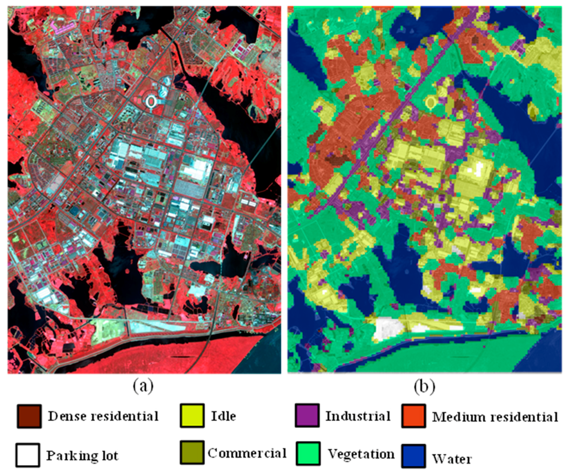
Figure 12.
The relationship between dropout rate and classification accuracy.

Figure 13.
The relationship between feature length L and classification accuracy.

Figure 14.
(a) The relationship between inf of the uniform distribution and classification accuracy. (b) The relationship between the standard deviation α of the Gaussian distribution and classification accuracy.
Figure 14.
(a) The relationship between inf of the uniform distribution and classification accuracy. (b) The relationship between the standard deviation α of the Gaussian distribution and classification accuracy.

Figure 15.
The class accuracy of the RssCNN, RotCNN and NrrCNN on the UCM.

Figure 16.
The class accuracy on OD and OD-8. (a) UCM dataset; (b) Google data of SIRI-WHU.

Figure 17.
The overall accuracy of the SRSCNN on the UCM and Google dataset of SIRI-WHU with different iterations.
Figure 17.
The overall accuracy of the SRSCNN on the UCM and Google dataset of SIRI-WHU with different iterations.


Table 1.
The main CNN structure configuration adopted in SRSCNN.
| Input (181 × 181 RGB image) |
| Conv3–32 |
| Conv3–64 |
| Maxpooling |
| Conv3–96 |
| Conv2–128 |
| Maxpooling |
| Conv3–160 |
| Maxpooling |
| FC-600 |
| Softmax |
Table 2.
Comparison with the previous reported accuracies with the UCM dataset.
| Classification Method | Classification Accuracy (%) | |
|---|---|---|
| Non-deep learning methods | BoVW | 72.05 |
| PLSA | 80.71 | |
| LDA | 81.92 | |
| SPCK++ [2] | 76.05 | |
| LLC [7] | 82.85 | |
| SPM+SIFT [7] | 82.30 | |
| SSBFC [7] | 91.67 | |
| SAL-PTM [10] | 88.33 | |
| DMTM [14] | 92.92 | |
| SIFT+SC [55] | 81.67 | |
| FK-S [56] | 91.63 | |
| Deep learning methods | M-DCNN [36] | 93.48 |
| S-UFL [37] | 82.72 | |
| GBRCN [40] | 94.53 | |
| LPCNN [41] | 89.90 | |
| CCNN | 91.56 | |
| SRSCNN-NV | 92.58 | |
| CNNV | 93.92 | |
| SRSCNN | 95.57 | |
Table 3.
Comparison between the previous reported accuracies with the Google dataset of SIRI-WHU, with 80% training samples selected.
Table 3.
Comparison between the previous reported accuracies with the Google dataset of SIRI-WHU, with 80% training samples selected.
| Classification Method | Classification Accuracy (%) | |
|---|---|---|
| Non-deep learning methods | BoVW | 73.93 |
| SPM-SIFT | 80.26 | |
| LLC | 70.89 | |
| LDA | 66.85 | |
| Deep learning methods | S-UFL [37] | 74.84 |
| LPCNN [41] | 89.88 | |
| CCNN | 88.26 | |
| SRSCNN-NV | 91.06 | |
| CNNV | 90.69 | |
| SRSCNN | 94.76 | |
Table 4.
Comparison between the published accuracies with the Google dataset of SIRI-WHU, with 50% training samples selected.
Table 4.
Comparison between the published accuracies with the Google dataset of SIRI-WHU, with 50% training samples selected.
| Classification Method | Classification Accuracy (%) |
|---|---|
| SSBFC [7] | 90.86 |
| DMTM [14] | 91.52 |
| LFK-Linear | 88.42 |
| FK-Linear | 87.53 |
| FK-S [56] | 90.40 |
| SRSCNN | 93.44 |
Table 5.
Comparison between the previous reported accuracies with the Wuhan IKONOS dataset.
| Classification Method | Classification Accuracy (%) |
|---|---|
| BoVW | 80.75 |
| LDA | 77.34 |
| P-LDA | 84.69 |
| FK-Linear | 78.23 |
| LFK-Linear | 79.69 |
| CCNN | 74.45 |
| SRSCNN-NV | 74.97 |
| CNNV | 79.60 |
| SRSCNN | 85.00 |
Table 6.
Sensitivity analysis in relation to the crop rate Cr.
| Dataset | Cr = 50% | Cr = 70% | Cr = 90% |
|---|---|---|---|
| UCM | 0.9486 | 0.9557 | 0.9398 |
| 0.9476 | 0.9468 | 0.933 |
Table 7.
Sensitivity analysis in relation to the spatial resolution.
| Dataset | OD | OD-4 | OD-8 |
|---|---|---|---|
| UCM | 0.9557 | 0.9500 | 0.9071 |
| 0.9476 | 0.9396 | 0.8958 |
© 2018 by the authors. Licensee MDPI, Basel, Switzerland. This article is an open access article distributed under the terms and conditions of the Creative Commons Attribution (CC BY) license (http://creativecommons.org/licenses/by/4.0/).
Share and Cite
MDPI and ACS Style
Liu, Y.; Zhong, Y.; Fei, F.; Zhu, Q.; Qin, Q. Scene Classification Based on a Deep Random-Scale Stretched Convolutional Neural Network. Remote Sens. 2018, 10, 444. https://doi.org/10.3390/rs10030444
AMA Style
Liu Y, Zhong Y, Fei F, Zhu Q, Qin Q. Scene Classification Based on a Deep Random-Scale Stretched Convolutional Neural Network. Remote Sensing. 2018; 10(3):444. https://doi.org/10.3390/rs10030444
Chicago/Turabian StyleLiu, Yanfei, Yanfei Zhong, Feng Fei, Qiqi Zhu, and Qianqing Qin. 2018. "Scene Classification Based on a Deep Random-Scale Stretched Convolutional Neural Network" Remote Sensing 10, no. 3: 444. https://doi.org/10.3390/rs10030444
Note that from the first issue of 2016, this journal uses article numbers instead of page numbers. See further details here.