Optimal Interpolation of Precipitable Water Using Low Earth Orbit and Numerical Weather Prediction Data

National Meteorological Satellite Center, Korea Meteorological Administration, Jincheon-gun 27803, Korea
*
Author to whom correspondence should be addressed.
Remote Sens. 2018, 10(3), 436; https://doi.org/10.3390/rs10030436
Submission received: 9 February 2018
/
Revised: 28 February 2018
/
Accepted: 5 March 2018
/
Published: 10 March 2018
(This article belongs to the Section Atmospheric Remote Sensing)
Abstract
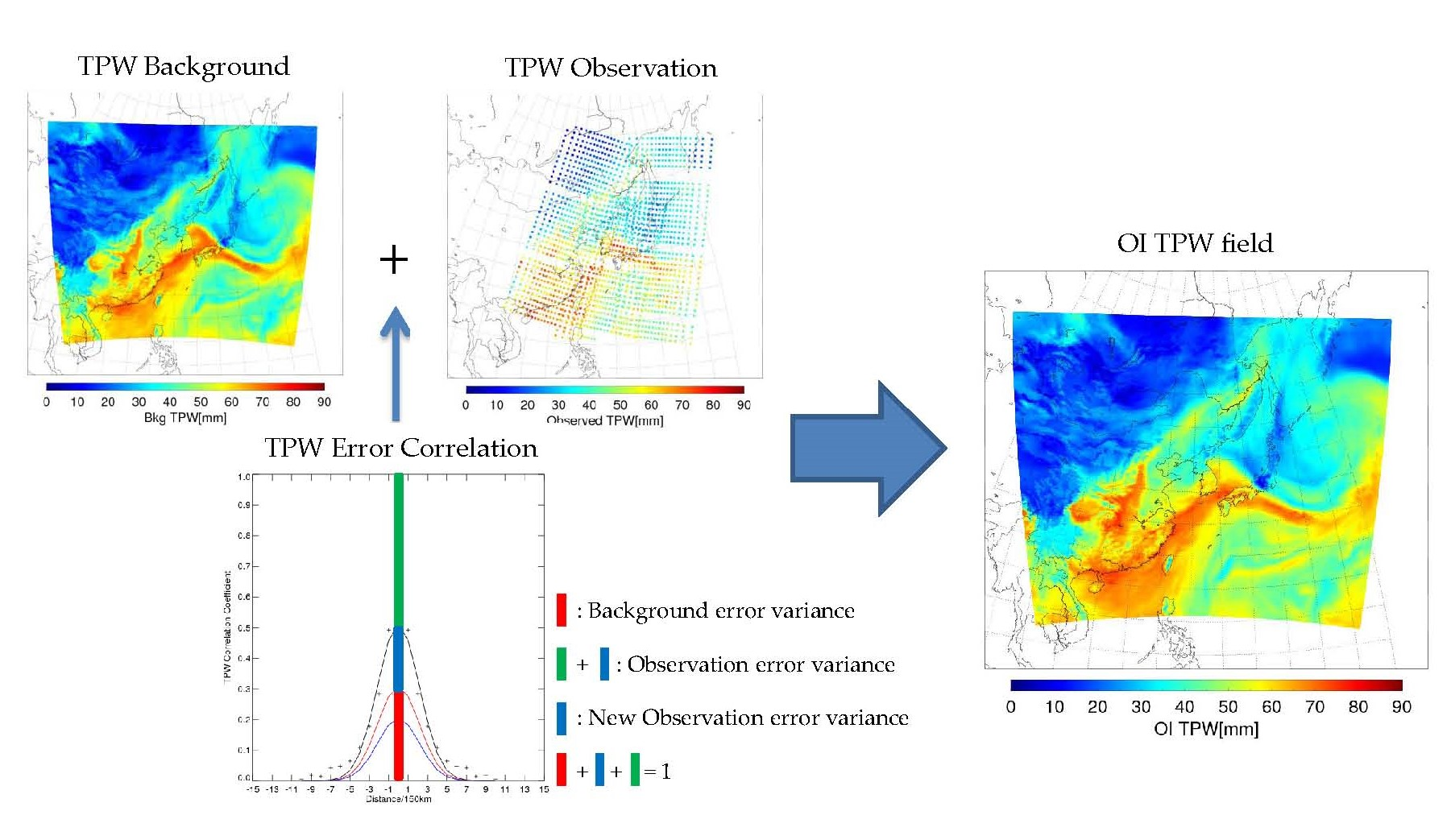
:The National Meteorological Satellite Center/Korean Meteorological Administration (NMSC/KMA) receives data directly from low Earth orbit (LEO) satellites (including NOAA-18,19; MetOp-A,B; and Suomi-NPP), and generates Level 2 products (e.g., temperature and humidity profile) in near real time. Total precipitable water (TPW) and layer precipitable water (LPW) are also generated using the retrieved humidity profiles. Today, forecasters need meteorologically-significant data fields composited from all available data sources, not multiple maps of observations from individual sources. Hence, TPW and LPW are reproduced using the optimal interpolation (OI) method with numerical weather prediction (NWP) data, in order to generate composite precipitable water (PW) products. In the OI procedure, PW data retrieved from the LEO satellites serve as observation data, while PW data from NWP serve as background data. Error covariances are estimated using a new approach, which considers correlations between observation errors to describe the characteristics of the errors better. Both background and observation error covariance matrices may have non-zero off-diagonal components. The composite PW products are validated using radiosonde data. The validation results for optimally-interpolated LPW (OI LPW) are much better than those for optimally-interpolated TPW (OI TPW). Generally, the OI LPW validation results are better than those for observation and background data; OI LPW data are ~5–10% more accurate than background data. Optimally-interpolated PW (OI PW) fields are applied to the correction of NWP forecast fields and the prediction of severe weather.

1. Introduction
It is vitally important to continuously monitor atmospheric phenomena in order to predict severe weather, such as torrential rain, and therefore reduce related damage. However, radiosonde sounding stations over land are limited; thus, atmospheric instability and precipitable water (PW) variations are continuously monitored using satellite observations. PW is used by forecasters to analyze severe weather events [1] and predict heavy precipitation [2]. Forecasters typically use a variety of data sources, from ground observations to numerical weather prediction (NWP). They prefer data fields blended from available sources during a given period of time to individual sources, in order to analyze synoptic phenomena [2].
The National Meteorological Satellite Center (NMSC) receives low earth orbit (LEO) observation data directly from satellites, such as the NOAA-18,19, MetOp-A,B, and Suomi-NPP, and produces Level 2 products in near real time, using LEO data processing packages [3,4,5], including the International Advanced Television and Infrared Observation Satellite Operational Vertical Sounder (ATOVS) Processing Package (IAPP), as well as the Community Satellite Processing Package (CSPP). In this study, humidity profiles and surface pressure data from these Level 2 products are used to calculate satellite-based PW, which are hereafter referred to as observation data. Temperature profiles, humidity profiles, and PW retrieved from ATOVS data from the NOAA-18,19 and MetOp-A,B satellites, using IAPP [3,4], all have 126 km 126 km resolution. Temperature profiles, humidity profiles, and PW retrieved from Cross-track Infrared Sounder (CrIS) sensor data from the Suomi-NPP satellite, using CSPP, have 41 km 41 km resolution. The assessment of the temperature and humidity profiles has been carried out in previous studies [3,4,6]. Also, the assessment of the satellite-based PW is carried out in Section 3.
The optimal interpolation (OI) method combines background and observation data to generate an analytical product that (1) covers stations without observations and (2) is more accurate than background and observation data, in terms of the root mean square error (RMSE) [7]. There are other methods suitable for the purpose of this study, such as kriging [8] and the cumulative distribution function (CDF) matching method [2,9]. The OI method has advantages over other methods, because it is not necessary to find out independent data [8] and reference data [2,9]. The OI method used in this study differs from other OI methods, in that we use non-zero off-diagonal components in the observation error covariance matrices. These non-zero off-diagonal components are obtained by estimating observation error variances and correlation length scales. Normally, a diagonal matrix is used for the observation error covariance matrix, because there is assumed to be no correlation between the two sets of observations [7,10,11]. This assumption does not hold true in this study, because the observation data should be correlated as they are observed, using the same instrument of the same satellite in an appropriate time window.
Section 2 describes the background and observation data and the OI procedure. A general method for calculating the correlation length scales and error covariances, as well as our new approach based on this general method, are also delineated in Section 2. The results of correlation length scales, error variances, optimally-interpolated PW (OI PW) fields, and validation are described in Section 3. Additionally, we discuss the relationship and independence of the data, error covariances, OI process for the upper layer, bias correction, and the operation of the OI process in near real time in Section 4.
2. Materials and Methods
2.1. Datasets
PW is calculated as the integral of the specific humidity q profile through a pressure layer divided by gravity in Equation (1) [1]:
PW is commonly expressed by forecasters in kilograms per square meter or in millimeters of condensate [1,2]. In this study, the PW variables are total precipitable water (TPW) and layer precipitable water (LPW), which consists of boundary layer (BL), middle layer (ML), and high layer (HL) precipitable water. TPW is the amount of water vapor in a column from the surface of the Earth to the top of atmosphere [2], and LPW is the amount of water vapor in a column from the chosen layer. BL, ML, and HL extend from the surface to 850 hPa, 850–500 hPa, and 500 hPa to the top of the atmosphere, respectively.
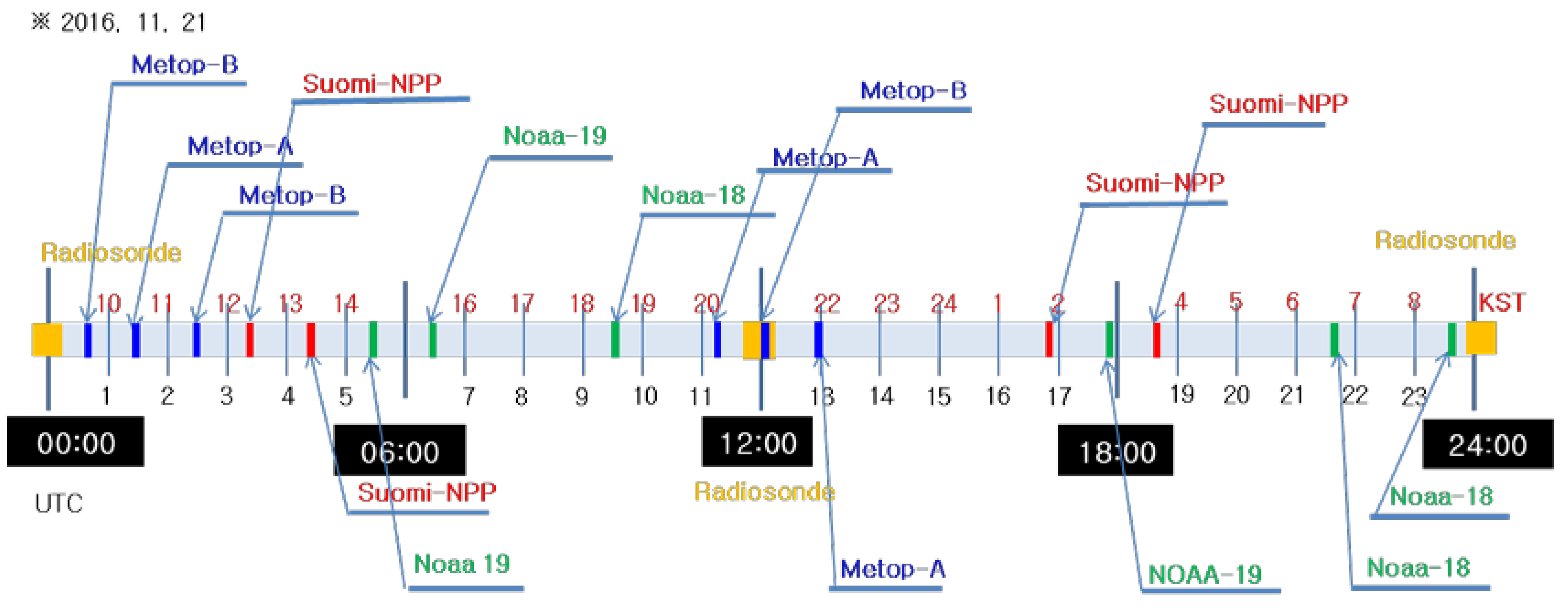
Satellite-based PW and NWP-forecasted PW fields are necessary for the generation of OI PW fields. On average, a satellite overpasses the Korean peninsula every hour and temperature (T) and humidity (q) are updated with the same frequency (Figure 1). T and q profiles from ATOVS have 126 km horizontal resolution and 1~2 km vertical resolution [4]. ATOVS consists of the High Resolution Infrared Radiation Sounder (HIRS), the Advanced Microwave Sounding Unit-A (AMSU-A) and AMSU-B. The Microwave Humidity Sounder (MHS) replaced AMSU-B on NOAA-19, MetOp-A, and MetOp-B. In the IAPP algorithm, AMSU-A measurements are remapped to HIRS field-of-view (FOV), and the retrieval processing is based on a field-of-regard (FOR) containing three by three adjacent HIRS FOVs [4]. An FOR from ATOVS is always defined as the three by three adjacent HIRS FOVs [4]. Because ATOVS uses a microwave observational platform, T and q profiles can be retrieved from ATOVS under all sky conditions (i.e., both clear and cloudy) [4]. Cloud detection and cloud removal procedure for HIRS are performed in IAPP [4]. CrIS T and q profiles have 41 km horizontal resolution and 1~2 km vertical resolution [12,13]. CrIS is an across-track scanning instrument with the total angular field of view consisting of a three by three array of circular pixels of 14 km diameter each (nadir spatial resolution) [13]. However, while T and q can also be retrieved from CrIS under all sky conditions, T and q profiles are only valid above the cloud top, because infrared cannot penetrate cloud. Thus, only clear-sky CrIS profiles are used to generate composite PW fields. Overpass time above the Korea peninsula, horizontal and vertical resolutions are summarized in Table 1.
The background PW data field is comprised of NWP q profiles, which are in turn produced by the Unified Model (UM) Regional Data Assimilation and Prediction System (RDAPS). The q profiles have 24 pressure levels; the UM RDAPS spans 491 segments at 12 km intervals from 101.58° E eastward, and 419 segments at 12 km intervals from 12.22° S northward [14]. Thus, RDAPS products including PW have a horizontal resolution of 12 km. The RDAPS generates 84-hour forecasts, with 3-hour intervals every 6 h (i.e., at 00:00, 06:00, 12:00, and 18:00 UTC). In this study, we use the 12-hour forecast field on average as background data in the OI process, because most weather forecasts refer to the 12-hour forecast field. In this paper, the relationship and independence of satellite-based PW and NWP-forecasted PW are discussed in detail in Section 4.1. The discussion is necessary for this OI study, because both satellite-based and NWP-forecasted PW data are generated from the data assimilation (DA) procedure.
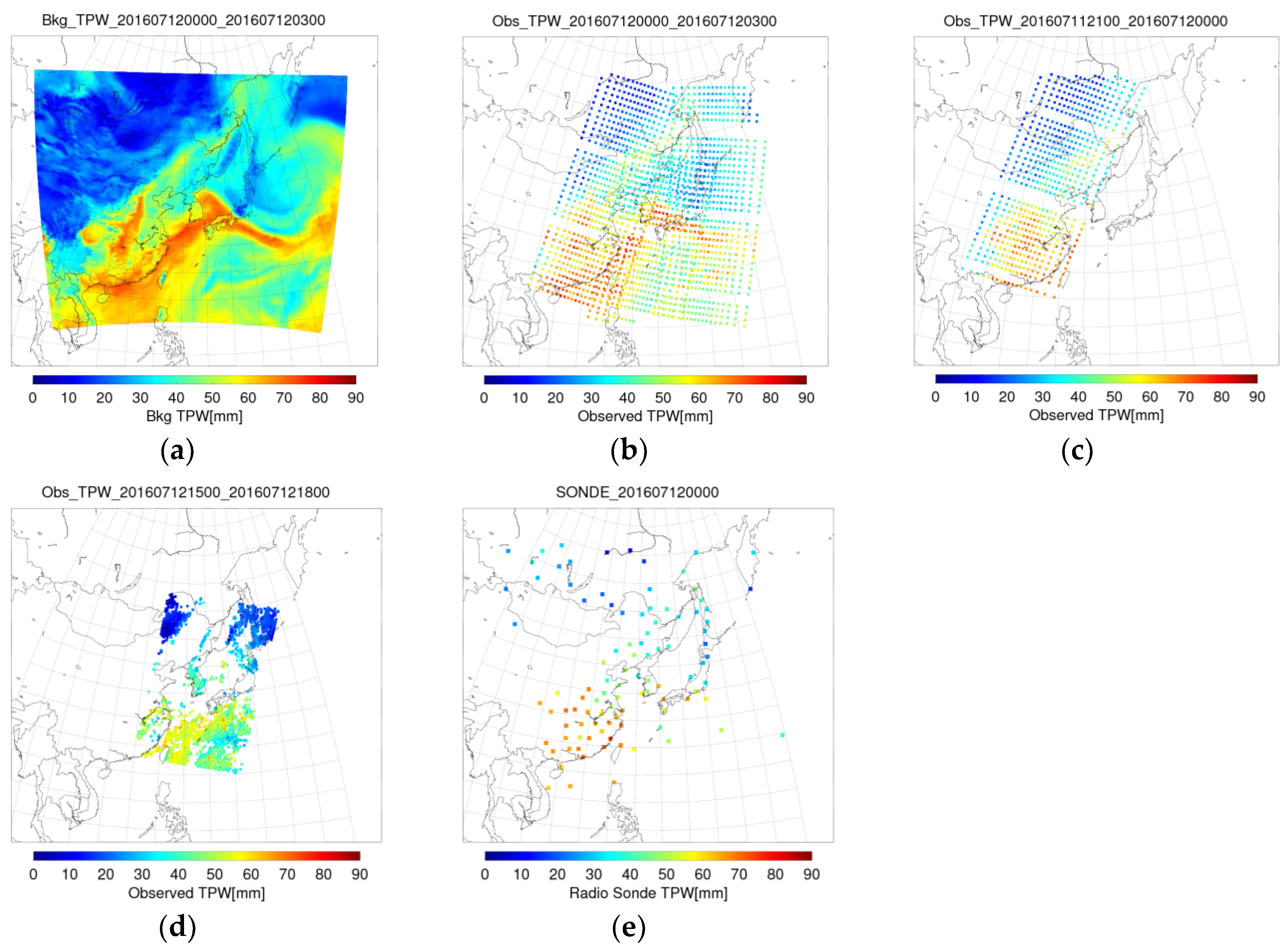
The background data used in the OI procedure were comprised of UM RDAPS-forecasted PW fields that were linearly time-interpolated using the central data, t + 12, and the additional forecast data, which are t + 9 or t + 15; here, t + 9, t + 12, and t + 15 mean 9, 12, and 15-hour forecast data. In Figure 2a, the time interpolation proceeds using t + 12 and t + 15, because this corresponds to the time period 00:00–03:00 UTC on 12 July 2016; here, t is 12:00 UTC on 11 July 2016. The time interpolation of the forecast data is operated to match the time of the background data to the observation data. The final background field is calculated by averaging the time-interpolated UM RDAPS-forecasted PW fields. The observation data are comprised of PW values retrieved from directly-received LEO ATOVS data from the NOAA-18,19 and MetOp-A,B satellites, and CrIS data from the Suomi-NPP satellite (Figure 2b–d). During OI analysis, background and observation data are artificially grouped into specific 3-hour time periods: 00:00–03:00, 03:00–06:00, 06:00–09:00, 09:00–12:00, 12:00–15:00, 15:00–18:00, 18:00–21:00, and 21:00–00:00 UTC; thus, eight OI PW fields are obtained during a day. Additionally, we use radiosonde data from meteorological agencies of the East Asia. Radiosonde data are used as the truth to validate the background, observation, and OI PW data. The basic radiosonde data are observed at 00:00 and 12:00 UTC, as shown in Figure 2e. The validation is based on radiosonde stations from the East Asia region.
2.2. Optimal Interpolation Procedure
Because OI is derived from a one-dimensional variation method, the OI method uses two datasets: the background dataset and the observation dataset. NWP forecast data were used as background data, primarily because these data are available in real time, and also fully filled with specific resolution for the given regions. In this study, the RDAPS 12-hour forecast and satellite-based PW were used as background and observation data, respectively, as mentioned previously. In the RDAPS field, the PW near regions where the satellite overpass was optimized, by combining NWP-forecasted and retrieved satellite PW data. We made several assumptions, including those related to non-trivial, unbiased, and uncorrelated errors, as well as linear and optimal analysis [15,16,17]. The definitions and explanations of the errors, and the basic notations used in this study are referenced using the previous papers [7,18,19,20].
The assumption of non-trivial errors implies that the background error covariance matrix () and observation error covariance matrix () are positive definite. The unbiased errors assumption means that background and observation errors are expected to be zero. The uncorrelated errors assumption suggests that the observation and background errors are not correlated. This assumption of uncorrelated or independent errors is discussed in detail in Section 4.1. The linear analysis assumes that the background corrections depend linearly on background observation departures, i.e., observation data minus a value calculated by applying the observation operator to the background data. The optimal analysis involves finding an analysis state that simulates the true state as closely as possible, in terms of RMSE (i.e., using a minimum variance estimate). Using the assumptions and techniques discussed above, the OI method sought to find a solution that minimizes the cost function [5,7,20,21,22,23].
Here is the background vector, which uses UM-forecast PW data; is the observation vector, which contains PW data retrieved from LEO data; is the observation operator; is the covariance matrix of the background errors; is the covariance matrix of the observation errors; and is the analysis vector that includes OI PW on the OI point. We considered that this cost function is for one PW variable. For example, the cost function for BL is constructed with only BL variables and their errors. , , and are comprised of BL data, with and comprised of BL errors. The dimensions of the vectors and the matrices determine the number of the horizontal points selected to perform the OI process. The selection of the points is described in Section 2.4, particularly in Figure 3c. If the dimensions of and are n and p, respectively, then the dimensions of , , and are p n, n n, and p p, where n and p are positive integers (1). In this study, n = p + 1 and the unit of background is the same as the observations (mm). Hence,
Here, p = 2 is an example to describe that the n = p + 1 relationship is established where the OI point has no observation data, while the other selected points have both background and observation data. Under these circumstances, the background vector dimension is equal to the observation vector dimension plus one.
If the probability density functions (PDF) of the background and observation errors are Gaussian, then is the maximum likelihood solution, because the probability of is equal to where is a positive constant [5,7,21,22,23]. From , we establish that ; thus, can be expressed in Equations (3) and (4):
is a linear operator and H = H in this study. Therefore is always satisfied [7,20]. and are described with components by components in the Section 2.3 and Section 2.4. The linear operator is the gain, or weight matrix, of the analysis [7,16].
2.3. Estimation of Error Variances
The correlation length scale is necessary for calculation of the off-diagonal components of the error covariance matrix, and can be estimated using the difference between observations and the background. The correlation length scale is not estimated directly from the observations [7,11]. Instead, within the assimilation system of interest here, the correlation length scale was estimated through the error covariances from the statistical analysis of the observation minus the background (O-B) with spatially homogeneous error variances [7]. Naturally, whenever error covariance is estimated, error variance is also estimated. The difference between the background error variance using the Hollingsworth–Lonnberg method [11] and the background error variance from this section is very important in the new approach presented in Section 2.4. If i and j are two observation points, and there is assumed to be no correlation between the background error and the observation error, the background departure (O-B) covariance is calculated as shown below [7,11].
In this study, the background and observation error variances are calculated by multiplying the O-B variance and the error variance ratio. The error variance ratio is given by
Here, and represent the background and observation error variances, respectively. and represent the ratios of the background and observation error variances. The observation and background data estimated at radiosonde observation (RAOB) stations using bilinear interpolation are not as accurate when they do not have a high resolution. The resolution of the background is 12 km, and that of the observation data is 45 km for CrIS and 126 km for ATOVS. These are not commonly considered high resolutions, implying that the background and observation error variances from the radiosonde validations are not as accurate. Therefore, the error variance ratio is considered approximately, as below.
and represent the background and observation error variances from RAOB, respectively. These are calculated by applying the bilinear interpolation to the background and observation data on the RAOB stations. Additionally, as shown in Equation (5), the O-B variance is the value of the variance of the observation error plus the variance of the background error. In Equation (5), the O-B variance is given as i=j.
Thus, the final variances in background and observation error are calculated by multiplying the O-B variance by the ratio of the error variance, as shown below.
Similarly, .
2.4. The New Approach: Considering Off-Diagonal Components
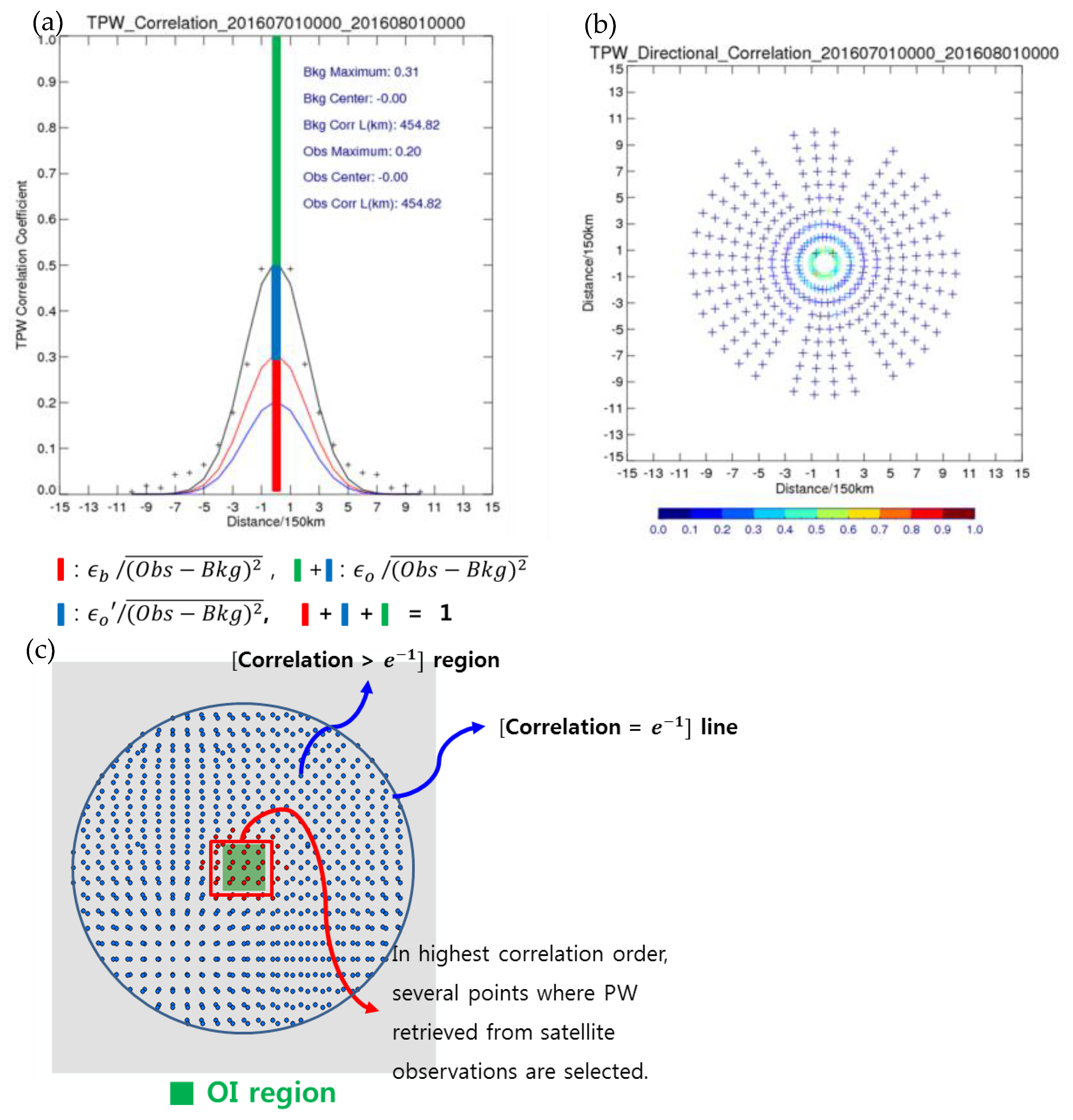
Under most O-B study methods, such as the Hollingsworth–Lonnberg method, retrieved PW satellite observation data must be uncorrelated with respect to distance. It is not possible to make this assumption when all of the retrieved PW data are used without loss, because correlations arise from initial guesses and data input to the regression procedure in the DA. Therefore, thinning of the retrieved PW data would be necessary in order to use the Hollingsworth–Lonnberg method. In this study, because retrieved PW data were used without loss, the discontinuity of the observation error covariance at distance = 0 was estimated more closely. In Equation (5), when which means that the observation errors are correlated with respect to distance. The background error variance was obtained using the Hollingsworth–Lonnberg method [7,11], and was greater than the background error variance, with calculated in this study due to the observation error correlations in the new approach. In Figure 3a, is shown over the scale of the correlation coefficient, adding the red and blue histograms when the distance was equal to 0. Here, is the new observation error variance (which describes the observation error covariance when distance > 0). A larger value indicates less observation error discontinuity when the distance was 0. As 0, the observation error covariance 0, and this new method approaches the Hollingsworth–Lonnberg method. Essentially, the Hollingworth–Lonnberg method results in the 0 case in Figure 3a. This means that the observation errors are uncorrelated with respect to distance, and when in Equation (5). Therefore was estimated to be by this method.
In the new method procedure, the first step is to check the PW variables for directional correlations (Figure 3b). The PW variables are nearly isotropic in most cases, so isotropic correlation length scales are assumed. If the directional tendencies are small or nonexistent, this isotropic assumption is maintained for simplicity. Next, we plot the O-B correlation coefficient with respect to distance. The distances in Figure 3a,b are between satellite observation points that involve collocated backgrounds. The black Gaussian function, which is calculated by a combination of the red and blue Gaussian functions, with maximum values of and at distance = 0, respectively, is fitted to the O-B correlation coefficient data with respect to distance (Figure 3a). Moreover, the correlation length scales of the background and observation error are assumed to be the same in the red and blue Gaussian functions for simplicity. The red Gaussian function represents the background error correlations with respect to distance, while the blue Gaussian function represents the observation error correlations with respect to distance, with the exception of distance = 0 (Figure 3a).
The OI boundary was selected using the Gaussian function of the background error correlations (Figure 3c). Here, the correlation coefficient is with respect to distance between the satellite observation point and the OI point; correlation is the boundary condition. Several satellite-observation PW retrieval points were selected in order from the point of highest correlation. In our module, a maximum of 50 satellite points could be selected.
If N satellite data are selected for use in OI, the error covariance matrices are constructed as below [7,18,19,20].
The components of the error covariance matrices are given in scalar, not vector notation. In this case, and represent errors at points i and j. is the background error correlation, which is a value on the red Gaussian in Figure 3a. is the observation error correlation, which is a value on the blue Gaussian in Figure 3a. is the of satellite , where refers to MetOp-A,B, NOAA-18,19, or Suomi-NPP. This is the same for and ; the other observation error components have the same notation. (the Kronecker delta) indicates that if which means the satellite types are the same, then . If which means that satellite types are different, then . The new approach produces the off-diagonal components, which are and in and . And the diagonal components are and as shown above.
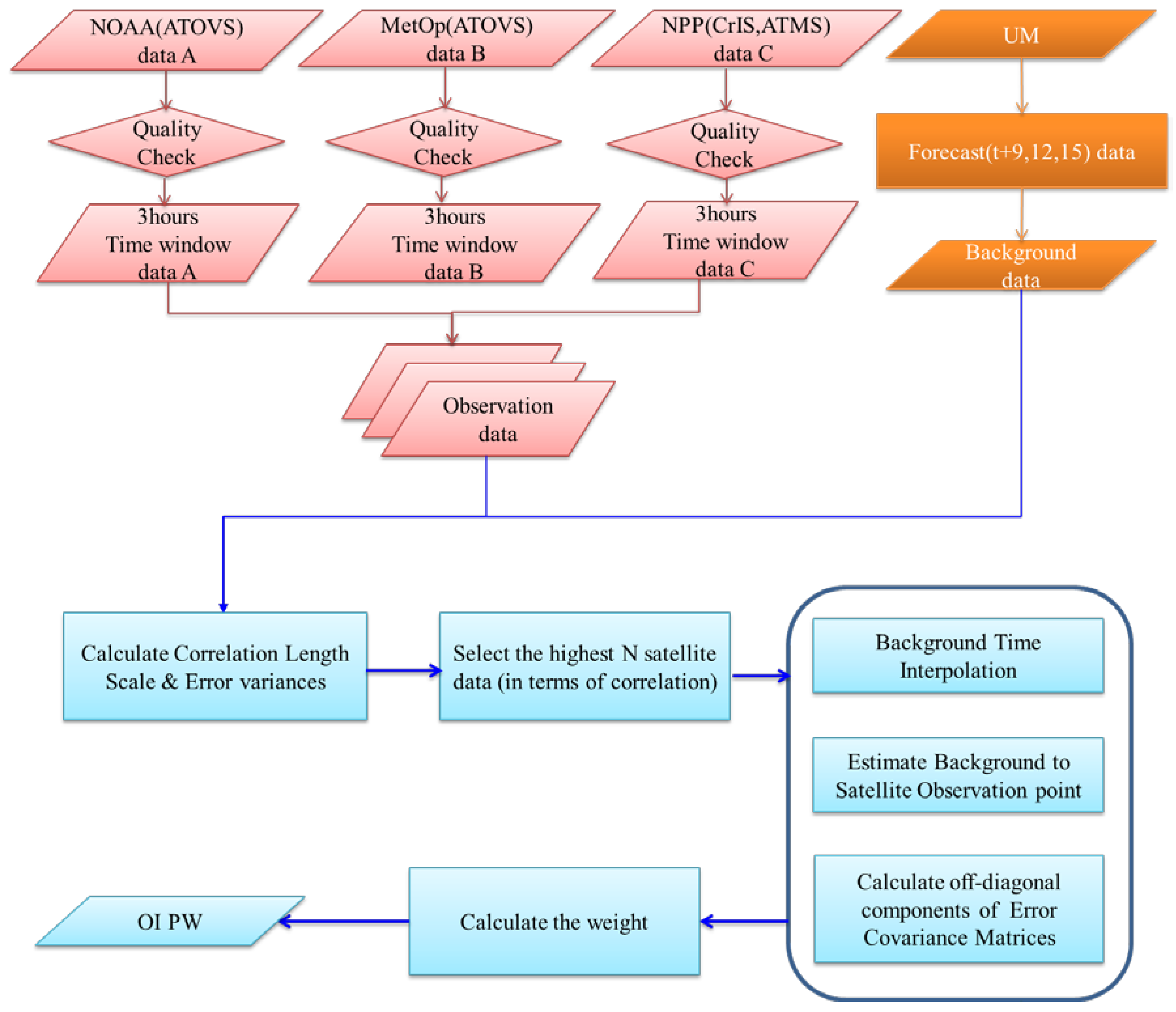
The whole OI process is described in Figure 4. First, using observation and background data, the correlation length scale and diagonal components of the background and observation error covariance matrices, the error variances are calculated. This process is the analysis of the error characteristics. After the first step, on the OI point, the N most highly correlated satellite data are selected, and the time-interpolated background field is generated. This background field is then used to estimate the background for the satellite observation points, by applying a spatial interpolation method involving bilinear interpolation to data near a given point. The off-diagonal components of the background and observation error covariance matrices are calculated using the correlation length scale, and these collocated background and observation data. The weight matrix is obtained using the constructed error matrices and the observation operator. Finally, OI PW is calculated by multiplying the weight matrix and the collocated O-B data.
3. Results
3.1. Correlation Length Scales and Error Variances
Using data from July 2016, correlation length scales and error variances were obtained for four PW variables for each satellite, as shown in Table 2. When OI was applied, the background error variance was
and the correlation length scale of the background error was
where and represent the and of the given satellite, and is the number of data from the satellite. Also , , and , which is set to be equal to , are the , , and of the given satellite. They were applied to each satellite data separately. And the factor, was multiplied by and to preserve and .
3.2. Optimal Interpolation Precipitable Water Fields
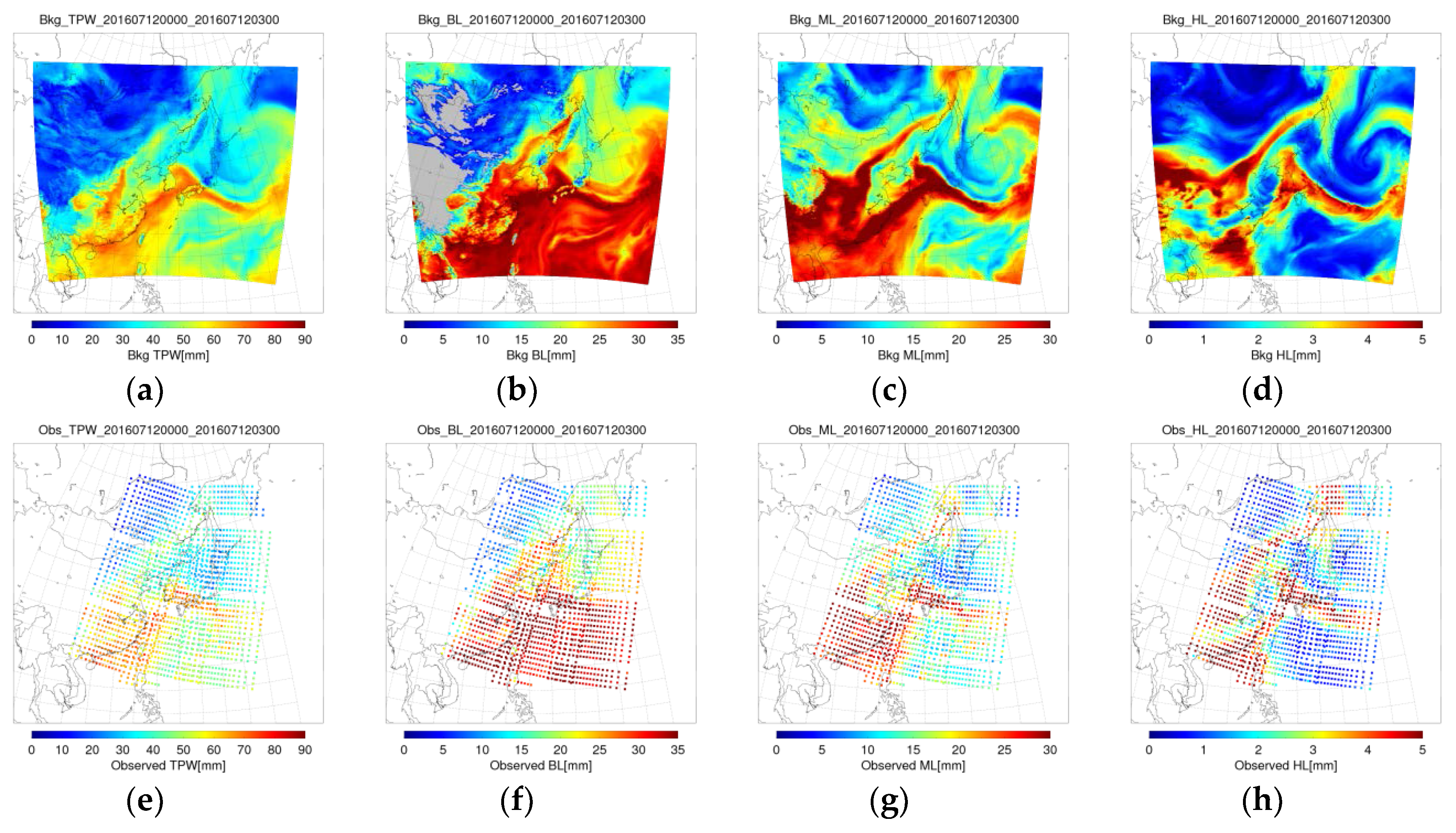
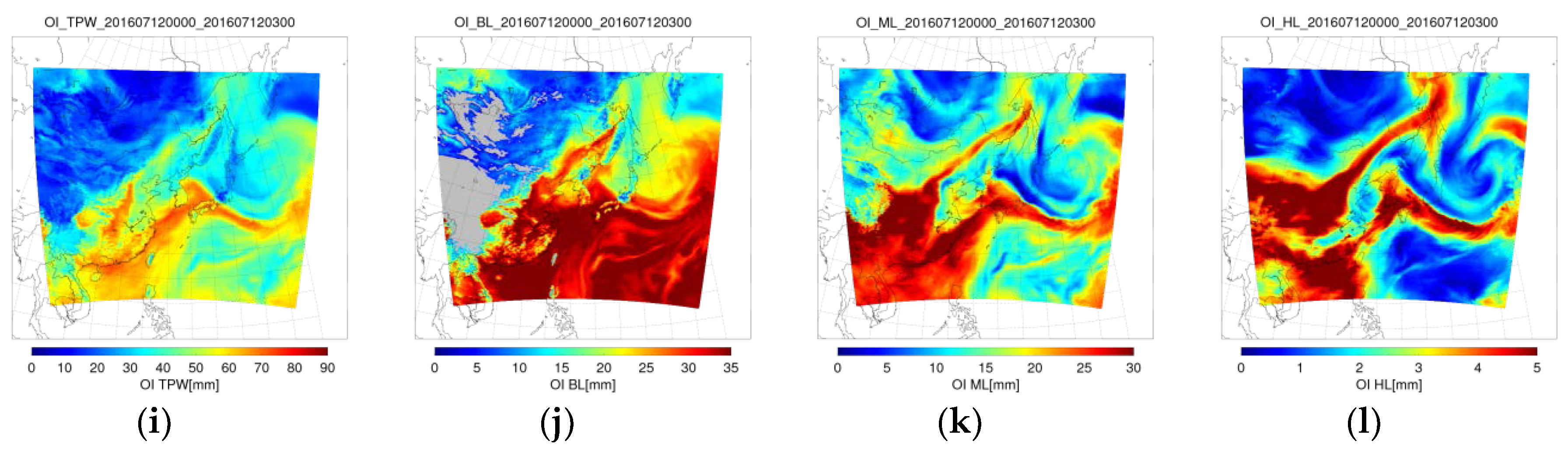
OI is operated using the correlation length scales and error variance data set, and OI PW fields are obtained as shown in Figure 5. Four OI PW fields, representing the OI TPW, BL, ML, and HL fields, were retrieved for specific 3-hour time periods throughout the day: 00:00–03:00, 03:00–06:00, 06:00–09:00, 09:00–12:00, 12:00–15:00, 15:00–18:00, 18:00–21:00, and 21:00–00:00 UTC. Also, using the difference between OI-background (OI-B) fields, information about correction of the background (NWP forecast PW fields) was obtained. This application is described in Section 4.4. The OI PW fields were obtained from Equation (3), the linear analysis [15,16,17] mentioned in Section 2.2. The OI-B increment in Equation (3) was calculated by multiplying the O-B column vector of the selected observation points with the weighting function calculated using the error covariance matrices and the observation operator. Hence, before quantitative validation, the OI PW fields were qualitatively validated via comparison with OI-B and O-B fields. Similarity between OI-B and O-B patterns indicated that the OI process works well (Figure 6).
3.3. Validation
Background, observation, and OI data of four PW variables were quantitatively validated using radiosonde data from the East Asia region, which were evaluated in terms of both the RMSE and bias. The validation period spanned 1 July 2016 at 00:00 to 1 August 2016 at 00:00 UTC. The results are shown in Table 3. The percentages in brackets indicate improvements made over background data through the application of OI. For example, the BL RMSE and bias were improved by approximately 7% and 62%, respectively, over the background BL values via the OI procedure. In this study, the radiosonde data of the same period were used to construct the error covariance matrices. The reason why the same radiosonde data were used in the validation is that the error characteristics of the validation period are described well when the data of the same period are used. However, this is not for operations in near real time. The analysis of the error characteristics for the operations in near real time are discussed in Section 4.5.
4. Discussion
4.1. Satellite-Based and Numerical Weather Prediction-Forecasted Precipitable Water Data
The OI PW data set were produced using satellite-based and NWP-forecasted data. It may be considered that updating the NWP DA schemes would be preferable to adding another layer. However, if NWP analysis data are used instead of NWP forecast data, temporal latency occurs. NWP analysis data are generated about four hours later than the times of observation data, such as satellites and RAOB [24,25,26,27,28]. In this study, NWP 12 h-forecasted were are used to avoid the latency. There are differences between forecast data and observation data [7,24,25,26,27,28]. Hence, the OI process is performed to effectively correct the differences, which are O-B.
The independency between satellite-based PW data and NWP-forecasted PW data must also be considered. This independency is related to the assumption of uncorrelated errors [15,16,17]. This assumption or hypothesis is usually applied because the causes of errors in the background and in the observations are supposed to be completely independent [7]. However, one must be careful about observation preprocessing practices (such as satellite retrieval procedures) that use the background field in a way that biases the observations toward the background, as this case may result in a suboptimal analysis [7]. In this study, satellite-based or satellite-retrieved PW data were used as the observation data; thus, this assumption should be considered carefully, because the analysis would be suboptimal. The result of the suboptimal case is clearly shown in OI TPW case. The assumption seems reasonable enough in OI BL and ML cases, as seen through the improved OI BL and ML validation results.
4.2. Error Covariance
The observation data are real time data, but the errors are larger than that of the background data which are NWP forecast data in the TPW, BL, and ML cases (Table 3). It may seem like the observation data has no clear benefits in the OI process. However, in the OI process, optimal data were produced through the analysis of the background and observation error characteristics [7,15,16,17]. In this process, the observation errors do not have to be smaller than the background errors. The important point is how accurately the errors are estimated in the OI process. Therefore, although observation data are not accurate in many cases, OI is useful with good estimations of the errors. This study is about the effect of the advanced error covariance structures on OI.
The OI PW seems to perform better in terms of RMSE than both background and observation data, because the optimal estimation method, which minimizes the cost function, is used in Equation (2). If the OI PW were to display a worse RMSE performance, it would indicate inaccurate error covariance of background and observation data. Table 3 indicates that the OI BL and ML perform better than the background and observation data, in terms of RMSE and bias. The OI HL performs better than both the background and observation data in terms of bias, but outperforms only the background data in terms of RMSE. These results indicate that the new approach to error covariance works well for the BL, ML, and HL. Improvements in the BL and ML are very useful to forecasters, because most of the water vapor in the atmosphere resides in the BL and ML. However, the OI TPW validation results are worse than the background and observation data, in terms of both RMSE and bias. Therefore, OI TPW was calculated in a different way, by adding OI BL, ML, or HL to background data of the remaining layers. However, the validation result of this case was also worse than both background and observation data. Therefore, TPW error covariance should be studied further in order to increase its accuracy. In this case, inflating the covariance of the observation error is necessary. Better validation results are obtained when the observation data are given less weighting, empirically, to validate the OI TPW. Firstly, the non-diagonal components of the observation error covariance matrix were considered, to inflate the matrix and give observation data a lower weighting in the cost function. In correspondence with these results, the TPW observation error covariances were estimated to be small in the OI process. However, physical or mathematical methods are not constructed enough. Therefore we need to study how much the observation error covariances are inflated, with reasonable methods.
Additionally, the summation of the background and observation error covariance can be calculated using Equation (5) without using truth, such as the radiosonde data. Equation (5) and the error covariance matrices used the unbiased errors assumption. The unbiased errors assumption means that both the background error and observation error are expected to be zero, as mentioned in Section 2.2. But this assumption does not mean that background or the observation data are true, because the zero means the average error for simple error covariance estimation [15,16,17]; thus, there are non-zero validation results for the background and the observation data, in terms of bias.
4.3. Optimal Interpolation Process for the High Layer
In this study, the use of radiosonde data is very important to determine the PW error characteristics. However, sometimes those data do not seem to be accurate in the upper troposphere and lower stratosphere, because radiosonde is driven by wind. Therefore, in the HL, it might not be appropriate to validate results and estimate error. The OI process for the HL should be studied further using other data, such as European Centre for Medium-Range Weather Forecasts (ECMWF) analysis data [23]. Radiosonde data are assimilated by NWP models, which are UM, ECMWF, and so on [24,25,26,27,28]. The satellite-retrieved product is validated using ECMWF analysis data in the previous study [29].
Fortunately, the HL represents a small portion of TPW. The amount of PW in HL is small compared to the BL and ML, and this is shown in vertical q profiles [4]. That fact suggests that inaccuracies in the HL rarely affect problems in the OI processes of the TPW. Additionally, radiosonde data were used to validate the whole of T and dew-point temperature profiles in the previous study [4]. The validation in this study is operated following the study.
4.4. Bias Correction
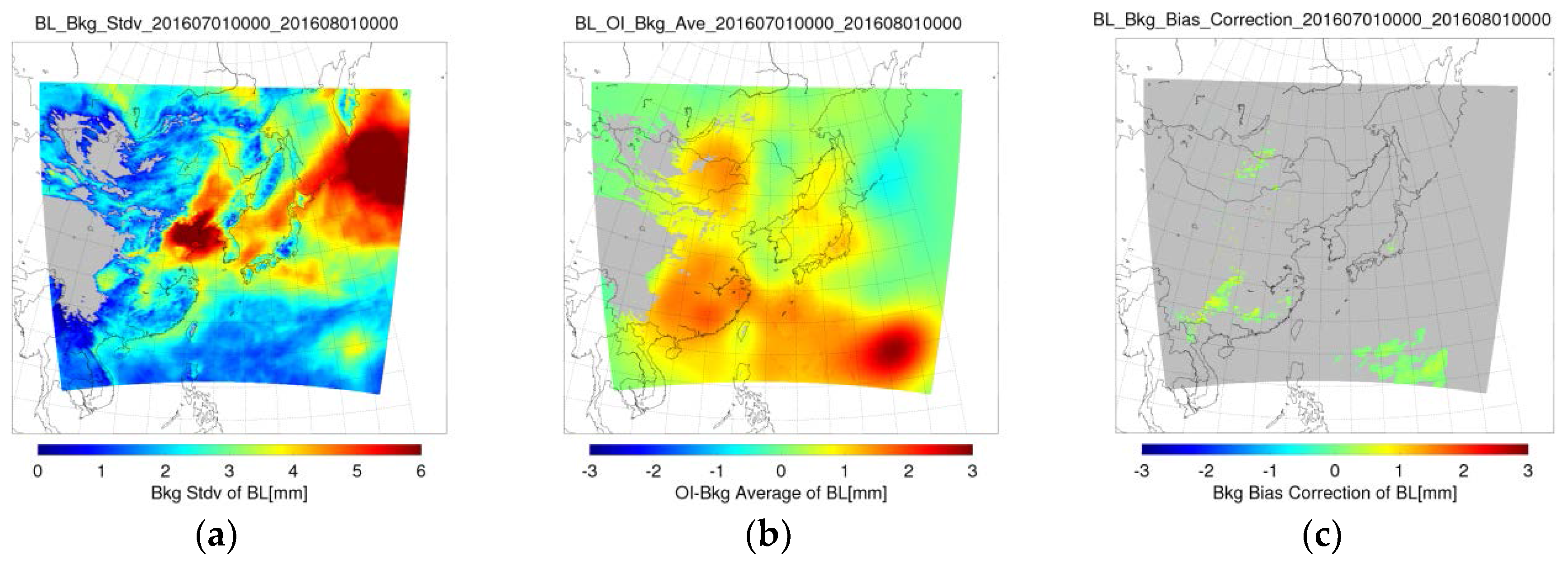
The background data (NWP forecast data) contain bias errors that should be reduced. The OI PW fields are applied to bias correction of the background fields. The monthly average of OI-B data is used to perform bias correction. Figure 7 shows an example of the BL bias correction. First, the background standard deviation (Bkg Stdv) is calculated (Figure 7a), in order to determine the valid bias region, defined as the region in which the absolute value of OI-B is greater than or equal to the absolute value of Bkg Stdv. Then, the OI-B is calculated (Figure 7b) and compared to Bkg Stdv, in order to find the valid bias region (indicated by colors other than gray in Figure 7c). The background PW is expected to be approximately within the background mean ± Bkg Stdv; thus, only the valid bias points are appropriate for use in background bias corrections. For these points, the bias correction applied to the background can be as large as − (Bkg Stdv), where 0 and + (Bkg Stdv), where < 0 during the selected period. Normally, the bias correction is applied to the PW variables, whose bias accuracy is improved by more than 50% compared to the background after the OI process. As mentioned in Section 4.2, the largest amount of water vapor is in the BL and ML. Bias correction of the BL and ML is therefore crucial for estimating accurate TPW, and predicting severe weather events such as heavy precipitation [1,2].
4.5. Operations in Near Real Time
For the operations in near real time, the seasonal or monthly error characteristics are assumed to rarely change as the years go by [23]. When OI PW fields are produced in near real time, the correlation length scales and error variances are recommended to be estimated using the data from the same month of the previous year, on the basis of the assumption of the rarely-changed error characteristics. Therefore, the background, observation, and radiosonde data from the same month of the previous year are used to construct the error covariance matrices in NMSC. The analysis of the error characteristics is performed once per month. The error information calculated are used for every OI process until the next calculation of the error information starts. Using the information, the OI TPW, BL, ML, and HL fields are retrieved every three hours (~00:30, ~03:30, ~06:30, ~09:30, ~12:30, ~15:30, ~18:30, and ~21:30 UTC). Four OI PW fields are retrieved every three hours, but this frequency can be changed depending on the run time of the OI procedure.
5. Conclusions
Using UM-forecasted PW data (at t + 9, t + 12, and t + 15) as background and LEO satellite-based PW data as observation, PW data were obtained over the UM RDAPS region using a new OI process. The OI-generated PW fields were more accurate than the background and observation data. In this OI procedure, correlation length scales and error variances were estimated via a new O-B fitting procedure that involved background and observation errors correlated with respect to distance. Then, error covariance matrices were constructed with non-zero off-diagonal components. The weighting function and OI PW fields were calculated using Equations (3) and (4), respectively. In this study, the OI TPW, BL, ML, and HL fields were retrieved for specific 3-hour time periods during a day: 00:00–03:00, 03:00–06:00, 06:00–09:00, 09:00–12:00, 12:00–15:00, 15:00–18:00, 18:00–21:00, and 21:00–00:00 UTC. Also, using OI-B fields, information about correction of the background was obtained from retrieved LEO PW. Both qualitative and quantitative OI PW validation were performed. Qualitative OI PW field validation involved evaluating similarities in O-B and OI-B patterns. In this study, these patterns were similar between the PW datasets. Quantitative validation involved the calculation of RMSE and bias in comparison to RAOB data for the period of July 2016. The OI BL and ML products performed better than the background and observation data in terms of RMSE and bias during July 2016. For the most part, OI LPW data (which can be further subdivided into OI BL, ML, and HL) performed better than both background and observation data, and the percentage improvement in OI LPW was higher than that in OI TPW. The OI PW data, which were much improved in terms of bias, were used to correct the background bias. Only the valid bias regions, in which OI-B values were greater than the standard deviation of the background, were used in this bias correction. When OI PW fields are produced in near real time, we recommend that the correlation length scales and error variances are estimated using data from the same month of the previous year, as data characteristics may vary with the season.
It is expected that familiarity with and application of OI PW will increase through continued OI development, allowing forecasters to use the improved imagery more efficiently with other meteorological data sets over East Asia [30]. Increased application will hopefully result in improved forecasts and lead times for precipitation, and especially heavy precipitation, which can result in flooding [2]. OI PW products can also be used to analyze severe weather events, such as floods and land-falling tropical depressions. Additionally, OI PW products have an advantage in tracking moisture over data-sparse regions under cloudy conditions, which makes them an ideal complement to geostationary satellite and radiosonde PW products [1]. On the OI point, the OI PW product is estimated using not the observation data of the point, but the observation data in the range of the correlation length scale from the point. Thus, the OI products under cloudy conditions do not suffer qualitatively. Additionally, the radiosonde data used for the validation were quality-controlled, so rare OI products are validated under convective conditions. We plan to use the truth data, such as ECMWF analysis data, to improve the validation process.
The OI procedure is also useful for the generation of other composite variables, such as sea surface temperature (SST) and aerosol optical depth (AOD). The OI procedure presented in this study is applicable to any variable that features one-to-one correspondence between the variable values and data points on a map, and for which “true”, observation, and background data are available. The OI procedure could be improved through further development of the analysis of the error characteristics. Currently, it is hard to say that there is a strong method to estimate both the background and observation errors accurately yet. If advanced methods are found, the OI procedure would be more powerful.
Acknowledgments
This research was supported by “the Development of Satellite Data Utilization and Operation Supportive Technology” of the NMSC/KMA.
Author Contributions
Jun-Hyung Heo conceived and designed the experiments; Jun-Hyung Heo performed the experiments; Jun-Hyung Heo, Eun-Ha Sohn, Geun-Hyeok Ryu analyzed the data; Jun-Hyung Heo and Eun-Ha Sohn contributed materials and analysis tools; Jun-Hyung Heo and Geun-Hyeok Ryu wrote the paper; Jae-Dong Jang managed the whole process of the research.
Conflicts of Interest
The authors declare no conflict of interest.
References
- Forsythe, J.M.; Kidder, S.Q.; Fuell, K.K.; LeRoy, A.; Jedlovec, G.J.; Jones, A.S. A multisensor, blended, layered water vapor product for weather analysis and forecasting. J. Oper. Meteor. 2015, 3, 41–58. [Google Scholar] [CrossRef]
- Kidder, S.Q.; Jones, A.S. A Blended Satellite Total Precipitable Water Product for Operational Forecasting. J. Atmos. Ocean. Technol. 2007, 24, 74–81. [Google Scholar] [CrossRef]
- Eyre, J.R. Inversion of cloudy satellite sounding radiances by nonlinear optimal estimation. I: Theory and simulation for TOVS. Q. J. R. Meteor. Soc. 1989, 115, 1001–1026. [Google Scholar] [CrossRef]
- Li, J.; Wolf, W.W.; Menzel, P.; Zhang, W.; Huwang, H.-L.; Achtor, T.H. Global Soundings of the Atmosphere from ATOVS Measurements: The Algorithm and Validation. J. Appl. Meteor. 2000, 39, 1248–1268. [Google Scholar] [CrossRef]
- Li, J.; Martinez, M.A.; Manso, M.; Velazquez, M.; Cuevas, G. Physical retrieval algorithm development for operational SEVIRI clear sky nowcasting products. In Proceedings of the 2008 EUMETSAT Meteorological Satellite Data User’s Conference, Darmstadt, Germany, 8–12 September 2008. [Google Scholar]
- Gambacorta, A.; Barnet, C.; Wolf, W.; Goldberg, M.; King, T.; Nalli, N.; Maddy, E.; Xiong, X.; Divakarla, M. The NOAA Unique CrIS/ATMS Processing System (NUCAPS): Fist Light Results. In Proceedings of the ITWG Meeting, Toulouse, France, 20 March 2012. [Google Scholar]
- Bouttier, F.; Courtier, P. Data assimilation concepts and methods March 1999. ECMWF. 2002, pp. 1–59. Available online: https://www.ecmwf.int/sites/default/files/elibrary/2002/16928-data-assimilation-concepts-and-methods.pdf (accessed on 10 March 2018).
- Schulz, J.; Lindau, R. Towards and Optimal Merging of Satellite Data Sets. 15 January 2014. Available online: https://www.researchgate.net/publication/228686783 (accessed on 24 February 2018).
- Lee, C.S.; Park, J.D.; Shin, J.; Jang, J.-D. Improvement of AMSR2 Soil Moisture Products over South Korea. IEEE J. Sel. Top. Appl. Earth Obs. Remote Sens. 2017, 10, 3839–3849. [Google Scholar] [CrossRef]
- Courtier, P.; Andersson, E.; Heckley, W.; Pailleux, J.; Vasiljevic, D.; Hamrud, M.; Hollingsworth, A.; Rabier, F.; Fisher, M. The ECMWF implementation of three-dimensional variational assimilation (3D-Var). Part 1: Formulation. Q. J. R. Meteor. Soc. 1998, 124, 1783–1807. [Google Scholar]
- Hollingsworth, A.; Lonnberg, P. The statistical structure of short-range forecast errors as determined from radiosonde data. Part 1: The wind field. Tellus 1986, 38, 111–136. [Google Scholar] [CrossRef]
- Smith, N.; Berndt, E.; Zavodsky, B.; Pierce, B.; Davies, J.; Hoese, D.; White, K.; Frost, G.; McKeen, S.; Wheeler, A.; et al. The Value of CSPP NUCAPS in Real-Time Applications. In Proceedings of the CSPP/IMAPP Users Group Metting, Madison, WI, USA, 27–29 June 2017. [Google Scholar]
- Shepard, M.W.; Cady-Pereira, K.E. Cross-track Infrared Sounder (CrIS) satellite observations of tropospheric ammonia. Atmos. Meas. Technol. 2015, 8, 1323–1335. [Google Scholar] [CrossRef]
- Numerical forecasting takes responsibility for the weather and climate industries!–Utilization guide of Numerical Weather Prediction model data for activation of the weather industry. Numerical Modeling Center of the Korea Meteorological Administration: Seoul, Korea, 2013; publication report number: 11–1360395-000252-01.
- Ghil, M. Meteorological Data Assimilation for Oceanographers. Part I: Description and Theoretical Framework. Dyn. Atmos. Oceans 1989, 13, 171–218. [Google Scholar] [CrossRef]
- Lorence, A. Analysis methods for numerical weather prediction. Q. J. R. Meteor. Soc. 1986, 112, 1177–1194. [Google Scholar] [CrossRef]
- Daley, R. Atmospheric Data Analysis; Cambridge Atmospheric and Space Science Series; Cambridge University Press: Cambridge, UK, 1991; p. 457. ISBN 0-521-38215-7. [Google Scholar]
- Hollingsworth, A.; Shaw, D.; Lonnberg, P.; Illari, L.; Arpe, K.; Simmons, A. Monitoring of observation and analysis quality by a data-assimilation system. Mon. Weather Rev. 1986, 114, 1225–1242. [Google Scholar] [CrossRef]
- Parrish, D.; Derber, J. The National Meteorological Center’s spectral statistical-interpolation analysis system. Mon. Weather Rev. 1992, 120, 1747–1763. [Google Scholar] [CrossRef]
- Ide, K.; Courtier, P.; Ghil, M.; Lorence, A.C. Unified Notation for Data Assimilation:Operational, Sequential and Variational. J. Meteor. Soc. Japan 1997, 75, 181–189. [Google Scholar] [CrossRef]
- Rodgers, C.D. Retrieval of atmospheric temperature and composition from remote measurements of thermal radiation. Rev. Geophys. Space Phys. 1976, 14, 609–624. [Google Scholar] [CrossRef]
- Li, J.; Huang, H.-L. Retrieval of atmospheric profiles from satellite sounder measurements by use of the discrepancy principle. Appl. Opt. 1999, 38, 916–923. [Google Scholar] [CrossRef] [PubMed]
- Martinez, M.A. Algorithm Theoretical Basis Document for “SEVIRI Physical Retrieval Product” (SPhR-PGE13 v2.0); AEMET: Madrid, Spain, 2013. [Google Scholar]
- Choi, Y.; Ha, J.C.; Lim, G.H. Inverstigation of the Effects of Considering Ballon Drift Information on Radisonde Data Assimilation Using the Four-Dimensional Variational Method. Weather Forecast. 2015, 30, 809–826. [Google Scholar] [CrossRef]
- Davies, T.; Cullen, M.J.P.; Malcolm, A.J.; Mawson, M.H.; Staniforth, A.; White, A.A.; Wood, N. A new dynamical core for the Met Office’s global and regional modeling of the atmosphere. Q. J. R. Meteor. Soc. 2015, 131, 1759–1782. [Google Scholar] [CrossRef]
- McGrath, R.; Semmler, T.; Sweeney, C.; Wang, S. Impact of balloon drift errors in radiosonde data on climate statistics. J. Clim. 2006, 19, 3430–3442. [Google Scholar] [CrossRef]
- Laroche, S.; Sarrazin, R. Impact of radiosonde balloon drift on numerical weather prediction and verification. Weather Forecast. 2013, 28, 772–782. [Google Scholar] [CrossRef]
- MacPherson, B. Radiosonde balloon drift—Does it matter for data assimilation? Meteor. Appl. 1995, 2, 301–305. [Google Scholar] [CrossRef]
- Martinez, M.A.; Romero, R. Validation Report for “SEVIRI Physical Retrieval Product” (SPhR-PGE13) v1.2; AEMET: Madrid, Spain, 2012. [Google Scholar]
- Kusselson, S.J.; Kidder, S.Q.; Forsythe, J.M.; Jones, A.S.; Zhao, L. An update on the operational implementation of blended total precipitable water. In Proceedings of the 23rd Conference on Hydrology, Phoenix, AZ, USA, 11–15 January 2009. [Google Scholar]
Figure 1.
Low Earth orbit (LEO) overpass time above the Korean peninsula.

Figure 2.
Datasets. (a) Background data comprised of UM forecast TPW; (b) MetOp-A,B (ATOVS) retrieved TPW data; (c) NOAA-18 (ATOVS) retrieved TPW data; (d) Suomi-NPP (CrIS) retrieved TPW data; and (e) Radiosonde data for the validation. The time periods for the NOAA-18 and Suomi-NPP data are different because there is no NOAA-18 and Suomi-NPP data for the time period used in (a,b).

Figure 3.
(a) Estimation of the correlation length scale and error covariances using the new approach in the scale of the correlation coefficient (July 2016 daily average); (b) isotropic assumption (July 2016 monthly average); and (c) optimal interpolation (OI) region selection. (a,b) are the NOAA-18,19 TPW product case.

Figure 4.
Optimal interpolation (OI) flowchart.

Figure 5.
For OI time period of 12 July 2016 00:00–03:00 UTC, (a–d) are background fields for four PW (TPW, BL, ML, and HL); (e–h) are observation data for four PW; and (i–l) are four OI PW fields.
Figure 5.
For OI time period of 12 July 2016 00:00–03:00 UTC, (a–d) are background fields for four PW (TPW, BL, ML, and HL); (e–h) are observation data for four PW; and (i–l) are four OI PW fields.


Figure 6.
Qualitative validation for OI time period of 12 July 2016 00:00–03:00 UTC. (a–d) are four OI-B PW fields; and (e–h) are four O-B PW data.
Figure 6.
Qualitative validation for OI time period of 12 July 2016 00:00–03:00 UTC. (a–d) are four OI-B PW fields; and (e–h) are four O-B PW data.

Figure 7.
An example of the valid bias region analysis (July 2016). (a) Bkg Stdv in the BL; (b) the expected OI-B in the BL; and (c) the valid OI-B region in the BL.
Figure 7.
An example of the valid bias region analysis (July 2016). (a) Bkg Stdv in the BL; (b) the expected OI-B in the BL; and (c) the valid OI-B region in the BL.


Table 1.
Overpass time above the Korean peninsula, horizontal and vertical resolutions for each satellite on 11 November 2016.
Table 1.
Overpass time above the Korean peninsula, horizontal and vertical resolutions for each satellite on 11 November 2016.
| Satellite | Overpass Time above Korea (UTC) | Horizontal Resolution (km) | Vertical Resolution (km) |
|---|---|---|---|
| MetOp-A | 01:24, 11:10, 12:56 | 126 | 1~2 |
| MetOp-B | 00:39, 02:25, 12:04 | 126 | 1~2 |
| NOAA-18 | 09:28, 21:41, 23:35 | 126 | 1~2 |
| NOAA-19 | 05:24, 06:30, 17:56 | 126 | 1~2 |
| Suomi-NPP | 03:25, 04:24, 16:57, 18:40 | 41 | 1~2 |
Table 2.
July 2016 correlation length scales and error variances for MetOp-A,B, NOAA-18,19, and Suomi-NPP. , , , , and have () unit. and have (km) unit.
Table 2.
July 2016 correlation length scales and error variances for MetOp-A,B, NOAA-18,19, and Suomi-NPP. , , , , and have () unit. and have (km) unit.
| Variable | , | |||||
|---|---|---|---|---|---|---|
| MetOp | ||||||
| TPW | 24.03 | 47.21 | 13.50 | 26.52 | 3.90 | 339.83 |
| BL | 13.32 | 20.50 | 4.88 | 7.51 | 0.00 | 636.37 |
| ML | 14.30 | 17.06 | 8.08 | 9.64 | 0.00 | 510.36 |
| HL | 1.25 | 0.90 | 0.60 | 0.43 | 0.00 | 981.69 |
| NOAA | ||||||
| TPW | 22.03 | 49.59 | 10.59 | 23.84 | 7.02 | 454.82 |
| BL | 13.88 | 22.32 | 4.52 | 7.27 | 0.00 | 636.37 |
| ML | 15.89 | 17.51 | 7.46 | 8.22 | 1.50 | 453.97 |
| HL | 0.94 | 1.05 | 0.40 | 0.45 | 0.03 | 657.07 |
| NPP | ||||||
| TPW | 20.06 | 83.41 | 15.31 | 63.67 | 21.83 | 636.37 |
| BL | 33.53 | 32.71 | 22.81 | 22.25 | 2.84 | 636.37 |
| ML | 14.43 | 18.41 | 11.45 | 14.61 | 1.82 | 751.08 |
| HL | 1.13 | 0.73 | 0.34 | 0.22 | 0.00 | 595.79 |
Table 3.
Quantitative validation over the period 1 July 2016 00:00–1 August 2016 00:00 UTC. (Left) PW RMSE; (Right) PW bias. The percentages in brackets indicate improvements made over background through the application of OI.
Table 3.
Quantitative validation over the period 1 July 2016 00:00–1 August 2016 00:00 UTC. (Left) PW RMSE; (Right) PW bias. The percentages in brackets indicate improvements made over background through the application of OI.
| Variable | RMSE (mm) | Bias (mm) | ||||
|---|---|---|---|---|---|---|
| Bkg | Obs | OI | Bkg | Obs | OI | |
| TPW | 3.58 | 5.11 | 3.79 | −0.23 | −0.21 | 0.30 |
| BL | 2.49 | 3.13 | 2.32 (6.91%) | −1.32 | −0.95 | −0.51 (61.75%) |
| ML | 2.85 | 3.09 | 2.73 (4.15%) | 1.69 | 0.08 | 1.21 (28.07%) |
| HL | 0.72 | 0.65 | 0.66 (8.00%) | −0.36 | 0.06 | −0.03 (91.19%) |
© 2018 by the authors. Licensee MDPI, Basel, Switzerland. This article is an open access article distributed under the terms and conditions of the Creative Commons Attribution (CC BY) license (http://creativecommons.org/licenses/by/4.0/).
Share and Cite
MDPI and ACS Style
Heo, J.-H.; Ryu, G.-H.; Jang, J.-D. Optimal Interpolation of Precipitable Water Using Low Earth Orbit and Numerical Weather Prediction Data. Remote Sens. 2018, 10, 436. https://doi.org/10.3390/rs10030436
AMA Style
Heo J-H, Ryu G-H, Jang J-D. Optimal Interpolation of Precipitable Water Using Low Earth Orbit and Numerical Weather Prediction Data. Remote Sensing. 2018; 10(3):436. https://doi.org/10.3390/rs10030436
Chicago/Turabian StyleHeo, Jun-Hyung, Geun-Hyeok Ryu, and Jae-Dong Jang. 2018. "Optimal Interpolation of Precipitable Water Using Low Earth Orbit and Numerical Weather Prediction Data" Remote Sensing 10, no. 3: 436. https://doi.org/10.3390/rs10030436
Note that from the first issue of 2016, this journal uses article numbers instead of page numbers. See further details here.