Estimating Live Fuel Moisture from MODIS Satellite Data for Wildfire Danger Assessment in Southern California USA

Abstract

The goal of the research reported here is to assess the capability of satellite vegetation indices from the Moderate Resolution Imaging Spectroradiometer onboard both Terra and Aqua satellites, in order to replicate live fuel moisture content of Southern California chaparral ecosystems. We compared seasonal and interannual characteristics of in-situ live fuel moisture with satellite vegetation indices that were averaged over different radial extents around each live fuel moisture observation site. The highest correlations are found using the Aqua Enhanced Vegetation Index for a radius of 10 km, independently verifying the validity of in-situ live fuel moisture measurements over a large extent around each in-situ site. With this optimally averaged Enhanced Vegetation Index, we developed an empirical model function of live fuel moisture. Trends in the wet-to-dry phase of vegetation are well captured by the empirical model function on interannual time-scales, indicating a promising method to monitor fire danger levels by combining satellite, in-situ, and model results during the transition before active fire seasons. An example map of Enhanced Vegetation Index-derived live fuel moisture for the Colby Fire shows a complex spatial pattern of significant live fuel moisture reduction along an extensive wildland-urban interface, and illustrates a key advantage in using satellites across the large extent of wildland areas in Southern California.

1. Introduction

Wildfires in Southern California (SoCal) are part of the natural cycle under Mediterranean climatic conditions. However, excessive urban growth in SoCal significantly increases the wildland-urban interface, and thus seriously compounds wildfire hazards, resulting in loss of human life and property [1,2]. Thus, improving fire danger assessment systems with a high spatial resolution and a wide coverage across the vast wildland is essential for decision makers and fire agencies to develop and implement pro-active policies. To assess wildfire danger, the United States Forest Service (USFS) has developed and utilized the National Fire Danger Rating System (NFDRS) [3], for which vegetation moisture is a key input.

While the moisture content of dead vegetation in NFDRS can be rather easily obtained from weather-dependent models since dead fuels are dependent on atmospheric variability [4], estimating the moisture content of live vegetation is more complicated because it depends on physiological properties that may significantly vary among different plant species [5]. To quantify moisture content of live vegetation, live fuel moisture (LFM) is defined as the percentage ratio of the difference between wet and dry weight to the dry weight of a vegetation sample [6].

In general, LFM is closely related to fire ignition, propagation, and intensity [7,8,9]. LFM has been incorporated into many fire behavior models (e.g., Fire Area Simulator or FARSITE model). Per Weise et al. [5], wildfire danger can be categorized with LFM levels (e.g., low: greater than 120%, moderate: between 80% and 120%, high: between 60% and 80%, and critical; less than 60%). Dennison et al. [9] have suggested that LFM lower than 77% appears to be historically associated with large fires in the Santa Monica Mountains of Los Angeles County, CA. Understanding seasonal trends of LFM can improve seasonal outlooks of LFM change and help to improve effective wildfire management as fire agencies operationally rely on field observations of LFM [6].

Currently, spatial coverage and temporal sampling of LFM data are severely limited as fieldwork for LFM measurements is labor intensive. LFM is manually measured weekly, biweekly, or monthly at a limited number of sampling sites across SoCal. For example, the Los Angeles County Fire Department typically samples LFM only at 11 disparate sites in its jurisdiction once every two weeks, leaving large data voids in areas where weather and geophysical variations can substantially affect LFM. In this regard, the capability of satellite data to observe LFM in each area around a given LFM site on a nearly daily basis, as compared to the weekly-monthly data from the manual method, can be a major advantage that is beneficial to fire agencies.

A potential approach to overcome the spatial and temporal limitations of manual measurements of LFM is to use vegetation indices (VIs) derived from satellite data. Satellite VI-based LFM estimations that have been attempted in the past were mostly for chamise ecosystems in California [10,11,12,13] and in Spain [8]. However, many studies were based on short-term records and statistical relationships without investigating seasonal and interannual characteristics of LFM and VIs based on obsolete satellite data collections with an inaccurate calibration.

Physically, LFM is dependent on precipitation, soil moisture, evapotranspiration, and the physiology of plants [6,14]. VIs retrieved from satellite remote sensing measurements are related to surface greenness and biomass of vegetation represented by the green leaf area index [15], which are impacted by and thereby correlated with LFM. Thus, VI and LFM are interdependent variables with similar seasonal and interannual trends, which suggest a possible estimation of LFM from remotely sensed VI. However, dissimilarities between them also exist. For example, plant growth requires not only moisture, but also optimal temperature and solar radiation, and vegetation moisture can also vary during the complex photosynthetic and xylem embolism processes in different plant species [16,17]. Therefore, to retrieve LFM from satellite VI data, it is necessary to conduct a careful investigation of LFM and VI characteristics by utilizing decadal datasets of in-situ and satellite measurements.

Previous studies have attempted to make a point-to-point comparison between LFM and VI or a combination of other VIs (e.g., [10,11,12,13]). Here, we examine the validity of multiple remotely sensed products used to estimate LFM, and thus we will investigate confounding factors and additional physical parameters necessary in the development of LFM model functions. Moreover, a review of past analyses raised concerns in remotely sensed LFM products [18]; however, many past results based on Moderate Resolution Imaging Spectroradiometer (MODIS) Collection 5 or earlier versions suffered from serious calibration problems [19,20], which caused significant errors in the remotely sensed VI products as recently published by Zhang et al. [21]. Such calibration problems necessitate a re-evaluation of the use of remotely sensed products to estimate LFM. Our novel approach is to test the LFM relationship with enhanced vegetation index (EVI) that is averaged over various spatial extents centered at each in-situ LFM sampling location. The objectives of this study are to: (1) Compare seasonal and interannual characteristics of LFM with those of VIs calculated from satellite data in SoCal; (2) develop an empirical model function of LFM based on an optimal vegetation index together with temperature data; and, (3) evaluate the feasibility, as well as limitations of the empirical model for wildfire danger assessments.

2. Methods and Materials

2.1. Live Fuel Moisture

Moisture content in live biomass is quantitatively characterized by LFM. LFM is defined as the percentage difference between wet and dry vegetation material over the dry mass of vegetation. Explicitly,

$$\mathrm{LFM}(\text{\%})=\frac{m_w-m_d}{m_d}\times 100,$$

(1)

where m_w is weight of the sampled vegetation, and m_d is the dry weight of the same sample. Our analysis was carried out primarily on chamise chaparral (Adenostoma fasciculatum), the most common shrub in the chaparral and regarded as an important fuel component in SoCal. The in-situ LFM dataset was obtained from the national live fuel moisture database (http://www.wfas.net/index.php/national-fuel-moisture-database-moisture-drought-103). LFM data are collected regularly every one or two weeks; however, the intervals can be longer during wet seasons when leaves and twigs remain wet after rainfall events. In these cases, fire agencies postpone their LFM sampling by a few days to avoid errors in LFM caused by excessive rainwater onto vegetation. To be compared to VIs, the LFM dataset was linearly interpolated at a daily time scale.

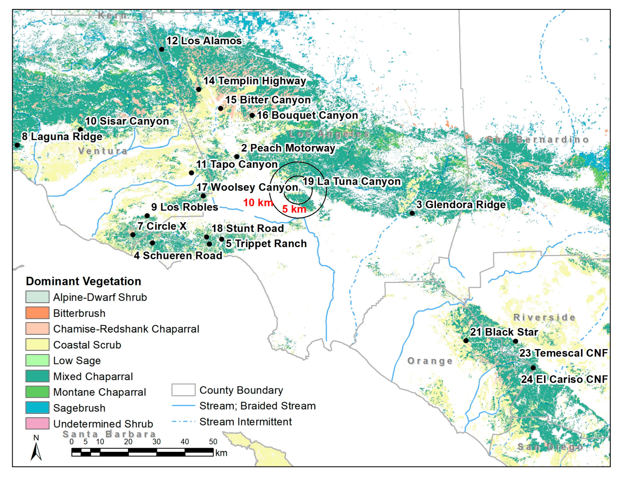
Among the 24 LFM sampling sites in Los Angeles, Ventura, and Orange County, 16 sites had data coverage for more than three years (

Table 1. Live fuel moisture (LFM) stations used in the study. Underlines indicate short names of the seven main research sites.

Name	Site Number	Latitude	Longitude	Fire Agency
Bitter Canyon	15	34.510000	−118.594444	LA County
Placerita Canyon	1	34.375278	−118.438889	LA County
La Tuna Canyon	19	34.246667	−118.302778	LA County
Laurel Canyon	20	34.124722	−118.368889	LA County
Trippet Ranch	5	34.093333	−118.597778	LA County
Schueren Road	4	34.078889	−118.644722	LA County
Clark Motorway	6	34.084444	−118.862500	LA County
Peach Motorway	2	34.355556	−118.534722	LA County
Bouquet Canyon	16	34.486111	−118.472778	LA County
Glendora Ridge	3	34.165278	−117.865000	LA County
CircleX	7	34.110833	−118.937222	Ventura County FD
Laguna Ridge	8	34.400000	−119.378889	Ventura County FD
Los Robles	9	34.171667	−118.882222	Ventura County FD
Tapo Canyon	11	34.306389	−118.710278	Ventura County FD
Sisar Canyon	10	34.447500	−119.135278	Ventura County FD
Black Star	21	33.754722	−117.670833	Orange County FD

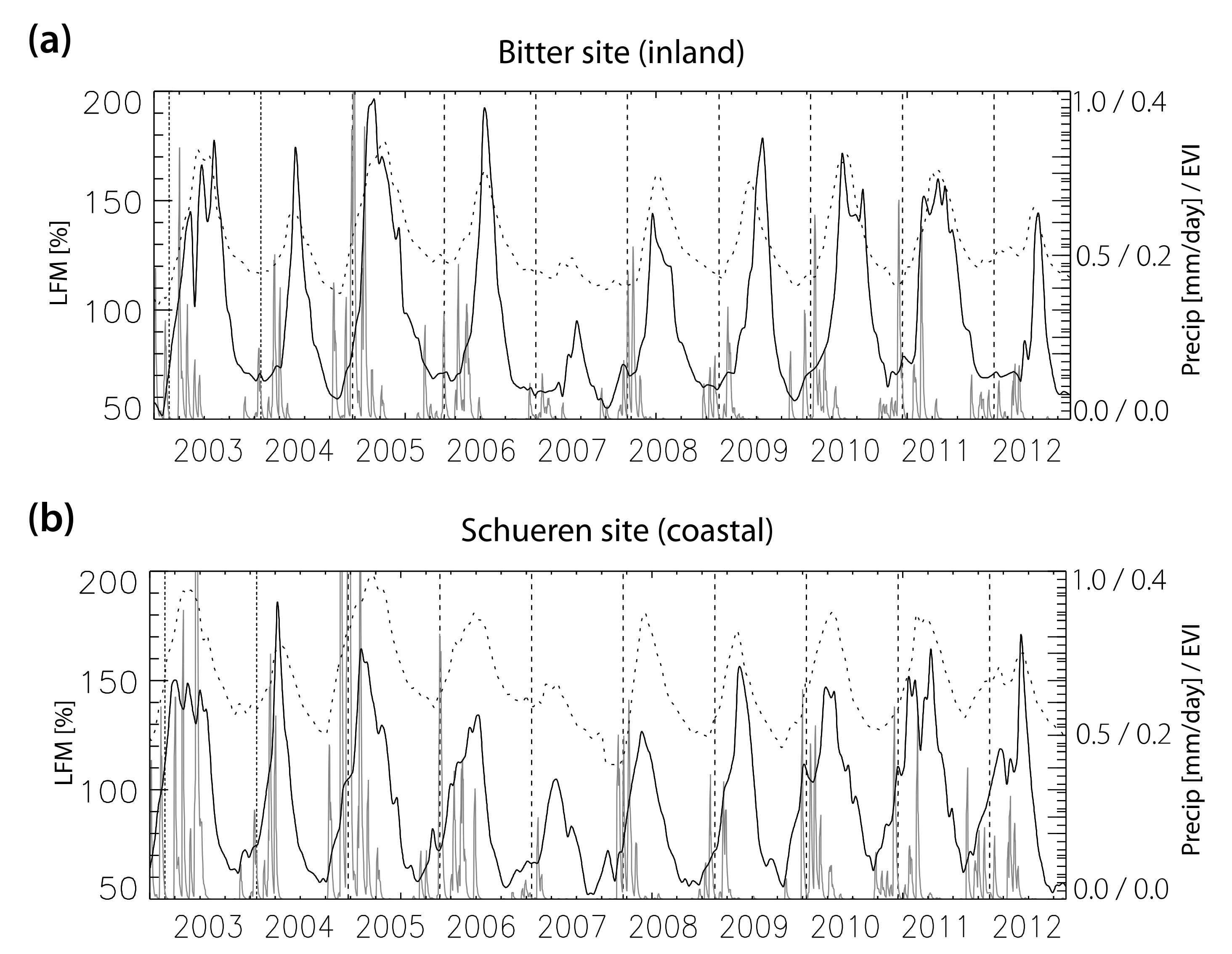
). The data from these 16 sites were selected for the regression analysis between LFM and VIs. For the longer-term analysis, data were selected from seven sites having more than 10 years of record from 2002 (bold characters in Table 1 and Figure 1). Four sites (Bitter, Placerita, La Tuna, and Laurel) were in inland areas (inland sites, hereafter), whereas the other three sites (Trippet, Schueren, and Clark) were in coastal areas (coastal sites, hereafter). Bitter and Schueren sites had corresponding meteorological stations, called Remote Automatic Weather Stations (RAWS); therefore, LFM and EVI comparisons with their corresponding atmospheric conditions were also investigated at these two sites. While utilizing LFM data at all of the sites to investigate and determine an overall universal LFM-EVI function may be desirable in principle, it is cautious that long-term data records at all the sites are required to ensure sufficient statistical sampling over the vast wildland in SoCal.

2.2. Remote Sensing Data

The present study focuses on the two most relevant VIs among an array of many VIs defined and used for different purposes: the normalized difference vegetation index (NDVI) and the EVI. NDVI and EVI were derived from the MODIS’ Vegetation Indices 16-Day L3 Global 250 m (MOD13Q1 and MYD13Q1)’ products from both the Terra and Aqua satellites [22]. The datasets were provided by the NASA EOSDIS Land Processes Distributed Active Archive Center (LP DAAC) at the USGS/Earth Resources Observation and Science (EROS) Center. The analysis period covered 10 years between October 2002 and September 2012, as VIs from MODIS have been available since 2001 for Terra and since 2002 for Aqua. We also investigated other VIs derived from MODIS land surface reflectance products (MOD09A1) for the same sites, including normalized difference water index (NDWI), normalized difference infrared index (NDII), and visible atmospherically resistant index (VARI) [23] (e.g., Table S1). These three VIs were recognized as effective indicators of vegetation water content and soil moisture [24,25].

To test the sensitivity of the LFM relationship with different areal averages of VIs, the values of the VIs were averaged over circular areal extents with various radii, ranging from 0.5 to 25 km. Then, the averaged VIs were used to correlate with LFM. This method allows for an independent assessment of the spatial extent where the in-situ LFM measurements are valid beyond the central sampling point. This is important because fire agencies intentionally select their LFM sampling locations to be representative of the surrounding vegetation conditions as far as possible so that measured LFM values are representative over an extensive area instead of being valid only at each sampling site. The sensitivity test results showed that a slightly higher correlation is observed at the 10-km radius (correlation coefficient of about 0.79) than that at 0.5-km radius (about 0.72 correlation coefficient). This suggests that a spatial average of VIs over a larger extent (~10-km radius) around each LFM location includes a larger ensemble of VI data, which statistically reduces satellite measurement noises as well as the effects of heterogeneous mixtures of different plant species within each sampling area. Thus, in this study, results for the areal extent of a 10-km radius, having the highest correlations, were selected to carry out the analysis.

2.3. Empirical Model

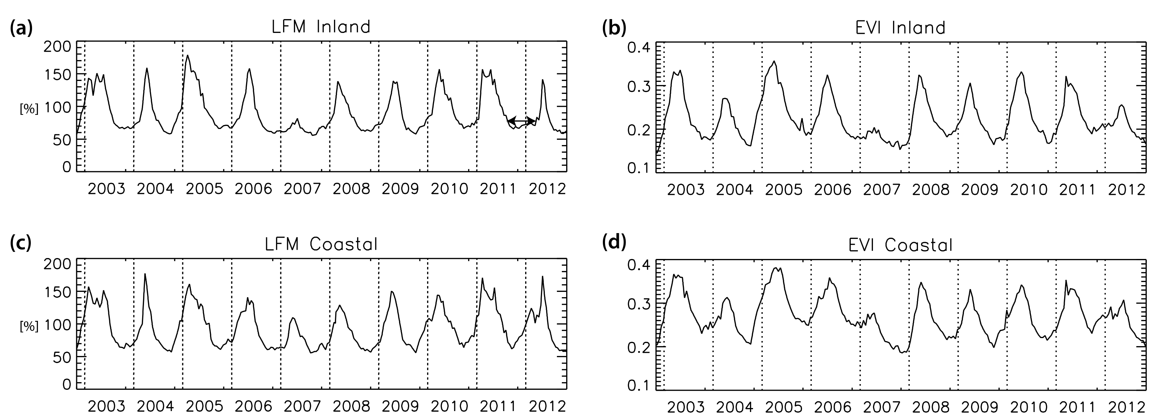
First, the Pearson correlation analysis is carried out to investigate the relationship between LFM and multiple VIs at 16 LFM sites to find the VI with the highest correlation against LFM. This VI is later employed as the major MODIS-derived indicator of vegetation water content for further analysis. LFM data available at the seven LFM sites in a 10-year period were separated into two different groups, representing the inland region and coastal region. Regional characteristics of LFM and EVI between inland and coastal regions were investigated together with their interannual variations. We then examined possible reasons for the different regional characteristics.

Next, linear regression models of VIs for LFM at the seven sites with decadal records were developed and evaluated across the 10-year data period with respect to the averages and inter-annual variability of maxima, minima, and transitional levels of LFM. We also tested non-linear models with a quadratic term or log transformation of the predictor, but a substantial improvement was not found. Therefore, in this study, two linear models are developed and tested. The first model uses each VI as a sole predictor (Equation (2)), while the second model includes a composite of collocated and contemporaneous VI and meteorological variables as predictors to account for the environmental dependence of LFM (Equation (3)), as follows:

LFM_i = β₀ + β₁ VI_i + ε_i,

(2)

LFM_i = β₀ + β₁ VI_i + β₂ MI_i + ε_i,

(3)

where MI is a meteorological factor with index i refers to various observations (i = 1, …, N), and ε_i is a residual error term.

VIs alone may not be sufficient to fully replicate LFM since using them is an indirect approach to infer the vegetation moisture. The other factors that were related to the dryness of vegetation conditions were selected for a test as an independent variable in addition to VIs. In this study, meteorological observations such as daily temperature (minimum, maximum and mean), relative humidity, and precipitation are chosen as additional variables in the composite estimation model. Due to large fluctuations in daily data, we used a 15-day running mean on LFM, EVI, and meteorological data in our analyses.

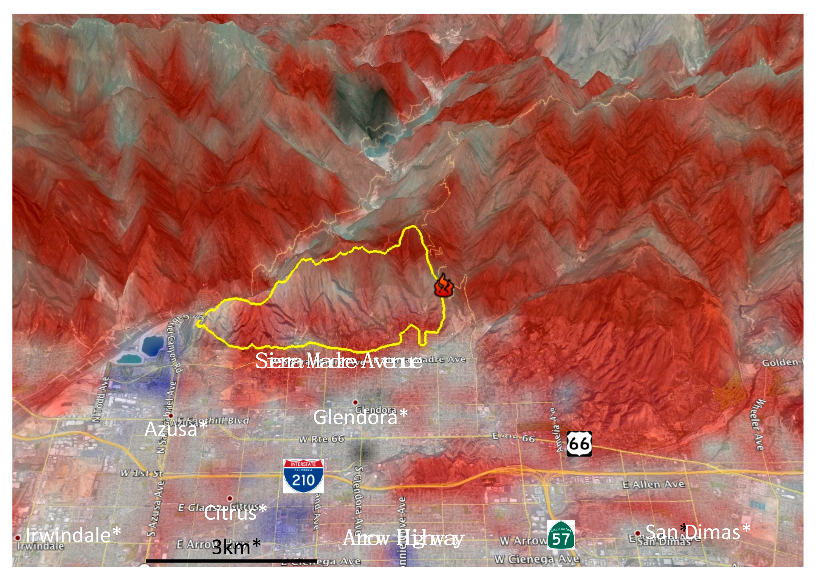
Finally, the capability of our satellite derived LFM model is tested in the case of the 2014 Colby Fire. The Colby Fire was ignited by an illegal campfire along the Colby Truck Trail in the San Gabriel Mountains of the Angeles National Forest on 16 January 2014 [26]. Fanned by dry and powerful Santa Ana winds, it burned over 1962 acres by 25 January at 98% containment. The fire destroyed five homes, damaged 17 other structures, injured one person, and forced an evacuation of 3600 people in the cities of Glendora and Azusa, California.

3. Results

3.1. Comparison of LFM and VIs

In-situ LFM and VIs showed similar interannual patterns with different amplitudes (Figure S1). Among the VIs, EVI showed the highest correlation (Figure S2). In fact, MODIS EVI was developed to enhance the sensitivity to a wider range of vegetation conditions and to improve vegetation monitoring through a decoupling of the canopy background signal and a reduction in atmospheric influences.

Regarding the difference between Aqua and Terra, the highest correlation to in-situ LFM was EVI derived from Aqua data when compared to the Terra data, and the lowest correlation with NDVI resulted from Terra data. In-situ LFM measurements were collected between 12 p.m.–4 p.m., spanning the local overpass time of Aqua (around 1:30 p.m.), while the data acquisition local time of Terra (around 10:30 a.m.) caused a mismatch with the timing of LFM sampling. Another issue was the gain drift problem in Terra data [19], which was corrected in MODIS Collection 6; however, the residual error remained larger in Terra products. Thus, we primarily used EVI from Aqua in the subsequent analyses in this paper.

Presented in Figure 2 are 10-year records of daily averaged LFM and the corresponding EVI at the coastal and inland sites. The results show distinctive differences between the two regional sites. For example, the moisture level of chamise at the coastal sites was higher than that at the inland sites, particularly in the moist-up phase (Nov-Apr) when LFM increased over the growing season (Figure 2a). Both coastal and inland LFMs attained their minima at the same time around the day-of-year (hereafter DOY) of 275. However, the coastal LFM reached its maximum earlier than that of the inland LFM, at DOY 87 and DOY 133, respectively.

Regarding EVI, the coastal EVI was consistently higher than the inland EVI, which was attributed to higher vegetation fractions at the coastal sites than those at the inland sites. The maxima occur almost simultaneously around DOY 105 in both regions, but date of minimum EVI at the costal sites was DOY 260, about 40 days earlier than that at the inland sites. While LFM exhibited strong variations in the moist-up phase, EVI had a more definitive peak toward the end of the growth period (Figure 2). These results reflected intrinsic differences between LFM and EVI characteristics.

The time series of LFM and EVI show significant interannual variations at both inland and coastal sites (Figure 3). Limited fuel moisture in chamise was most prevalent in 2007, and the vegetation at the inland sites experienced a greater moisture deficit than that at the coastal sites. In contrast, there was relatively higher fuel moisture in 2003 and 2005. Similar features were consistently found in EVI in both wet and dry years. In addition to the overall pattern, EVI also replicated the differences of LFM between the inland and coastal sites; e.g., higher LFM values at the coastal sites as compared to those at the inland sites during the 2011–2012 winter.

The time series also reveal different interannual characteristics of LFM and EVI (Figure 3). First, LFM showed higher values of maxima for most years, even during dry years, except for 2007. For example, during the two dry years, 2004 and 2012 (77% and 27% winter precipitation received with respect to the 1950–2000 mean, respectively), maximum LFM values were close to those in wetter years. In these two years, the start of LFM growth period was delayed and began decreasing earlier, and these changes induced an enhanced kurtosis shape of the LFM time series, and vice versa in the wetter year. The variations in the LFM kurtosis were more pronounced at the inland sites. When compared to LFM, the kurtosis of EVI did not vary substantially, but maximum values fluctuated more interannually, while the rate of EVI seasonal change did not have a strong variation from year to year.

Minimum values of LFM stayed in the 50% range even in dry years (e.g., 2004, 2007, and 2012), albeit that EVI value dropped below normal in those years. Near minimum LFM values at the inland sites continued for seven months during the 2011–2012 fire season (e.g., the arrow in Figure 3a). The persistently low LFM values occurred as the plants sustained a minimal level of moisture for survival by tightly closing their stomata during dry and hot summers to minimize water loss through transpiration [8]. While there was an overall similarity in seasonal and interanual behavior of LFM and EVI, detailed differences in LFM and EVI characteristics would contribute to the uncertainty when estimating LFM from EVI to be discussed in the next section.

To investigate the responses of LFM and EVI to precipitation, we overlaid a time series of precipitation on the LFM and EVI records at Bitter (one of the inland sites) and Schueren (one of the coastal sites) as presented in Figure 4. The intensity and timing of rainfall were closely related with LFM behaviors. LFM started to increase after rainfall and peaked in early summer. LFM showed minimum in fall until rain would start in the next winter. When compared to the Bitter site, the precipitation rate at Schueren was higher and attributable to the higher levels of LFM in fall and winter. Minute amounts of precipitation in 2007 and 2012 caused abnormally low LFM. These results suggested that LFM would directly respond to the water availability from rainfall.

EVI exhibits similar characteristics as LFM, except for a delayed response to initial precipitation events in some years. For example, there was a tendency for an increase of LFM prior to an increase of EVI in the early wet season, supported by consistent negative values of the difference between minimum LFM dates and minimum EVI dates, as shown in Figure 5a, for the difference of minimum dates (LFM-EVI). Ranging from −4 to −123 days, this pattern was observed in 68% of the cases at the Bitter and Schueren sites and more obvious at Schueren. When precipitation in a rainy season is significantly reduced, and thus seasonality of LFM becomes vague, the minimum date difference tends to be large (e.g., 2007/08 and 2012/13 cases in Schueren). Regarding the maxima, the timings of the EVI maxima were slightly earlier or later without any consistent bias of sign, compared to those of the LFM ranging from −39 to +68 days (Figure 5b). These results indicate that EVI captures the general seasonal trend of LFM. However, the discrepancy in the timing of minimum and maximum of EVI and LFM suggested that additional factors would be necessary in combination with EVI to accurately capture the seasonal behavior of LFM.

3.2. Empirical Model for LFM Estimation

A linear regression model relating LFM to EVI, termed an empirical model function (EMF), was developed at each site, and the results are shown in

Table 2. Results of the linear regressions between LFM and EVI.

Site Name	Coefficient (β1)	Constant (β0)	R2	Significance
Bitter	477.93	−3.98	0.73	<0.001
Placerita	669.43	−49.67	0.76	<0.001
La Tuna	538.50	−42.72	0.79	<0.001
Laurel	501.36	−38.76	0.70	<0.001
Trippet	468.59	−27.74	0.65	<0.001
Schueren	479.77	−33.36	0.67	<0.001
Clark	475.74	−27.73	0.74	<0.001

. With EVI as a single predictor, constants and coefficients of the EMF were similar among several different sites. Figure 6a,c present time series of in-situ LFM and EVI-based estimates at Schueren and Bitter, respectively. These results highlighted the overall consistency across the 10-year period between in-situ LFM and EVI-estimated LFM. However, because of the significant discrepancies in the maxima and minima, it was necessary to quantitatively evaluate the performance of the EMF in characterizing 10-year averages and interannual variability of the timing, as well as in obtaining magnitudes of maxima and minima. In addition, the date when LFM reached 90% level was also examined. The 90% LFM value represents a transitional stage that approaches high fire danger and an active fire season [5].

Table 3. 10-year mean of differences between estimation and in-situ LFM for value and date of maximum and minimum LFM, and date of 90% LFM value at each site.

Site Name	Maximum LFM		Minimum LFM		90% LFM
	Value (%)	Date (Day)	Value (%)	Date (Day)	Date (Day)
Bitter	−16.7	−0.7	1.6	17.4	1.2
Placerita	−20.5	−16.2	1.8	10.3	−6.8
La Tuna	−10.7	1.1	1.0	28.8	−3.1
Laurel	−13.5	−3.0	0.5	26.9	−5.5
Trippet	−15.3	5.2	4.2	22.8	9.2
Schueren	−16.7	−6.7	7.0	42.7	1.5
Clark	−15.4	12.0	5.6	2.4	−4.9

represents the differences (estimated LFM minus in-situ LFM) of the 10-year mean values at each site. The results showed that the EVI-based model underestimated maximum LFM values by 10–20% when compared to in-situ LFM. The differences of the date of maximum LFM were usually less than 16 days without any systematic bias in signs, which were consistent with the lack of any systematic bias in the maximum dates of LFM and EVI (Figure 4 and Figure 5). In contrast, EVI slightly overestimated minimum values by 0–7% of the in-situ LFM. Nevertheless, the differences in the minimum dates were significant (2~43 days), corresponding to the temporal lag or delay in EVI minima as compared to that of in-situ LFM minima.

With regards to the 10-year correlation (

Table 4. Interannual correlations between the estimated and in-situ LFM with respect to values and dates of maximum and minimum of LFM, and 90% LFM. Asterisks (*) indicate statistically significant correlations at the 95% confidence level.

Site Name	Maximum LFM		Minimum LFM		90% LFM
	Value	Date	Value	Date	Date
Bitter	0.84 *	0.45	0.32	0.57	0.85 *
Placerita	0.79 *	0.19	0.72 *	0.69 *	0.72 *
La Tuna	0.66 *	0.63 *	0.48	0.34	0.61 *
Laurel	0.70 *	0.82 *	0.42	0.12	0.78 *
Trippet	0.44	0.82 *	0.53	0.42	0.69 *
Schueren	0.27	0.71 *	0.63 *	−0.20	0.80 *
Clark	0.35	0.69 *	0.78 *	0.69 *	0.87 *

), interannual maximum values of in-situ LFM were significantly correlated with those of the estimates only in the inland regions (Bitter, Placerita, La Tuna, and Laurel) at the 95% confidence level. For the minimum values, only three sites (Placerita, Schueren, and Clark) showed statistically significant correlations. With respect to dates, the maximum dates of in-situ LFM matched well with those of the EVI-estimates for most of the sites, but minimum dates did not, as indicated by the low or negative correlation coefficients at most of the sites, except Placerita and Clark. These results reflected limitations of the EMF using EVI alone to replicate extrema (especially minima) in LFM values and dates.

Regarding the issue of the underestimation of LFM maxima, a contributing factor was the small interannual variation observed in the maximum values of in-situ LFM (i.e., the large variations of LFM kurtosis in Figure 3) when compared to those of the EVI. The small variation in in-situ LFM maxima was likely a consequence of the LFM sampling practice of fire agencies during wet seasons; that is, when it rains during the period, the two-week interval of LFM measurements was often delayed by a few days to avoid errors that are caused by rainwater-residue on plants during or after rainfall events. Therefore, when fire agencies measure LFM after rainfall, LFM values were generally larger as the time delay allowed more absorption of ample moisture from precedent rainfall. As a result, high values of the LFM maxima were consistently observed for most of the years except for excessively dry years, such as 2007. In contrast, EVI is responsive to canopy physiological variation rather than just vegetation moisture. Furthermore, EVI values are less sensitive to precipitation owing to the spatial averages across large areas where precipitation may occur in different subsectors at different times. Because of the combined effects of these two factors, it is likely that LFM more directly and rapidly reacts to precipitation compared to the EVI response.

Our results also indicate that the estimation error of the EMF for minima is not negligible. Two reasons likely responsible for these limitations were: (1) The presence of the threshold of minimum LFM value (e.g., 50% range), unlike the behavior of the EVI; and, (2) the delayed increases of EVI when compared to LFM in early transition into the growing season, as presented in the previous section. In contrast, the 90% dates were well identified by EVI at all of the sites with respect to both the 10-year mean and variability. The 10-year average differences of the 90% dates were less than 10 days without any systematic bias (Table 3). As a result, the interannual correlations between the 90% LFM date and the corresponding estimates from the EMF were consistently and significantly high.

We also examined correlations between the modeled LFM and in-situ LFM where changing periods of the in-situ LFM reached at 100 to 70% (

Table 5. Interannual correlations between the estimated and in-situ LFM with respect to of the dates of various LFM thresholds. Asterisks (*) indicate statistically significant correlations at the 95% confidence level. The highest correlation among the four LFM thresholds at each site is indicated in bold.

Site Name	Dates of In-Situ LFM Thresholds
	100%	90%	80%	70%
Bitter	0.78 *	0.85 *	0.81 *	−0.03
Placerita	0.64 *	0.72 *	0.68 *	0.90 *
La Tuna	0.58 *	0.61 *	0.78 *	0.60 *
Laurel	0.62 *	0.78 *	0.68 *	0.40
Trippet	0.68 *	0.69 *	0.80 *	0.69 *
Schueren	0.67 *	0.80 *	0.59 *	−0.29
Clark	0.91 *	0.87 *	0.92 *	0.64 *

). The highest correlations at each site ranged between 0.78 and 0.92 and occurred at either a 90% or 80% wet-to-dry transitional threshold except at Placerita. The 90% and 80% LFM are related to the moderate or high fire danger levels in the 10-year analysis period, the dates of these thresholds varied significantly year to year. Therefore, the high correlation results validated a considerable capability of the LFM EMF to capture the dry vegetation transition into the high fire danger range. A previous study had pointed out that 77% of LFM is a threshold for large historical wildfires in SoCal [27]. This would indeed support that EVI-based estimations in this study could provide valuable information for determining the actual start dates of a fire season and potential dangers of large wildfires.

3.3. Modified Empirical Model Using Temperature

As indicated in the previous section, EVI alone might not be sufficient to fully replicate LFM due to other factors that are involved in causing dryness of vegetation conditions. To improve the LFM EMF, we tested the EMF model using several meteorological variables from RAWS station as an independent variable in addition to EVI. The results indicate that among the daily temperatures, humidity, and precipitation, the model improvement was highest with the use of daily minimum temperature (T_min) (Table S2). It is notable that daily maximum and average temperature and humidity also result in the model improvement, while daily precipitation does not. The EMF using both EVI and T_min at Schueren is described in

Table 6. Results of the linear regressions of LFM at Schueren.

Independent Variable	Coefficient (β1, β2)	Constant (β0)	Significance	R2
EVI	478.801	−32.9543	<0.001	0.68
EVI, Tmin	429.641, −1.100	40.5482	<0.001	0.73

. The inclusion of T_min together with EVI substantially improved the results, especially for lower values (Figure 6 and Figure 7), although the improvement in term of R² was not large.

In our modified EVI-T_min model, the coefficient of T_min was negative (−1.1), implying that a higher temperature was associated with lower LFM value for the same values of EVI. This suggested two possible processes that could be responsible: (1) Leaves closed their stomata under extremely hot conditions and surface temperatures consequently increased due to a lack of transpiration from the leaves [8]; and/or, (2) plants lost their moisture under hot and dry weather conditions through evaporation at their stomata or on the surface of their leaves. Anyway, the additional information carried in the minimum air temperature variable certainly enhanced the model performance, especially in the dry season. This is also supported by the closer association of the EVI-T_min derived values with the one-to-one line than that of the EVI-alone derived values (Figure 7a,b), especially for drier conditions, represented by LFM values lower than 110%.

Furthermore, wet-to-dry transition timing is better related to the EVI-T_min estimation. For example, 80% dates from the EVI-T_min estimation were better correlated with those from in-situ sampling than those from the EVI-alone estimation (Figure 7c). In particular, the EVI-alone model failed to detect the 80% date in 2006 and 2007, as the EVI-alone estimated LFM values that were were higher than 80% during the entire wet-dry season. In contrast, the EVI-T_min model significantly reduced errors in identifying the 80% date in 2006 and 2007 when compared to the results from the EVI-alone model. EVI-T_min model is also better suited for monitoring the transitional levels of LFM.

The improvement attained by adding the temperature variable was not uniform. For example, adding temperature as an additional independent variable at the Bitter site only slightly improved the performance of the EMF. Nevertheless, as low values of LFM signify higher fire danger levels, any improvement in the estimation of LFM, especially during dry seasons, can be valuable in enhancing the capability for fire danger assessment.

3.4. Applying LFM Model to a Real-Life Wildfire Case

The capability of satellite EVI to replicate LFM presented a potentially powerful methodology that could enable daily LFM observations over vast wildland areas in SoCal as well as similar climatic regions that are prone to wildfires around the world. Such capability would set forth a new era for fire danger assessment, one that uses satellite-estimated LFM validated by in-situ LFM. These data products enabled an improvement of more than one order of magnitude of temporal and spatial coverage as compared to the labor-intensive, manual methods currently conducted by fire agencies in their standard bi-weekly in-situ LFM sampling at sparsely selected local locations.

To demonstrate the satellite utility for LFM observations, the real-life case of the 2014 Colby Fire is highlighted as an example here. A quantitative measurement of LFM changes between 25 February 2013 and 8 January 2014 was illustrated over the regional topography in three dimensions, as shown Figure 8. This type of measurement was derived from Aqua MODIS EVI based on the EMF at Glendora Ridge, located within the burned area, i.e., LFM = (417.602 × EVI) + 6.78061. The EMF was developed in the same manner as EMFs were developed in Table 2, except using a nine-year dataset. This is due to the substantial amount of LFM data missing at Glendora Ridge in 2005. The red areas, pervasive mostly in the mountains, corresponded to a sharp decrease of over 80% in LFM on 8 January (Figure S3) from an LFM level of 140% on 25 February 2013. This happened during the 2013 fire season, which was anomalously prolonged into the first quarter of 2014 due to the severe winter drought of California in 2013 and 2014 [28]. Such a drastic plunge in LFM took the normally pre-fire season LFM levels in January in 2014 to below 60% by the week before the Colby Fire ignited. Note that 60% LFM would be considered the critical fire danger level [5] as being used by fire agencies to implement pro-active fire preparedness measures.

The ignition point (flame symbol, Figure 8) of the Colby Fire was located on the east side of the fire perimeter (yellow contour, Figure 8) within vegetation with critically low LFM values, as observed by MODIS. Fortunately, the Colby Fire did not spread to many critical danger areas around the immediate vicinity due to the aggressive firefighting efforts of the Los Angeles County Fire Department (LACoFD). The LACoFD proactively decided to extend its normal fire season, typically ending around December, due to the extremely low LFM values that were measured throughout the wildlands in the county. The road network overlaid on the satellite LFM map (Figure 8) highlights the encroaching urban growth from several cities (Irwindale, Citrus, Azusa, Glendora, and San Dimas) sprawling into the Los Angeles County wildland. Note that Interstate 210, Route 66, and Route 57 clearly intersect the rough terrain where satellite LFM indicated critical red fire danger levels. This kind of map could be very useful for the National Weather Service (NWS), as well as for local fire agencies in SoCal for fire danger assessment in real-life operational environments. It could also be used by the commercial and private sectors, such as electric utility companies who might have power lines running over critical wildlands, and everyday homeowners who could use such a map to readily check their addresses for potential wildland fire danger in their local community [29].

4. Discussion

In this study, we have analyzed climatological, seasonal, and interannual characteristics of LFM and satellite VIs in SoCal in order to develop empirical model functions of LFM based on VIs together with air temperature data based on statistical analyses. Correlation results between LFM and various VIs indicated that LFM was most strongly correlated with EVI from Aqua. Unlike previous studies attempting a point-to-point comparison, we tested the LFM relationship with EVI averaged over different areal coverages in chamise-dominant grids (i.e., 0.5 km to 25 km radius circles), and found that LFM was well correlated with EVI averaged over large areas. It was most strongly correlated with the area of a 10-km radius centered around each in-situ LFM site. As LFM measurements represented information over a large spatial extent, LFM could have high correlations between the time-series data records at different locations as indicated in the high cross correlations. In addition, we found that the higher the cross correlation, the longer the distance between the LFM sampling sites (Table S3). This was an independent verification that measured LFM values at in-situ sites, strategically selected by fire agencies, are indeed a good representation of moisture levels over the extensive neighboring area.

A possible explanation of the better correlation between EVI and LFM is the co-varying leaf pigment concentrations with the change of vegetation water content in Southern California [18]. When plants are under water stress, depletion of chlorophyll may produce a decrease in reflectance in visible and NIR bands. Such change can be prominent in Mediterranean plants as they have a quick response under dehydration. This change may produce a stronger signal than the response in SWIR bands due to the change of vegetation water content.

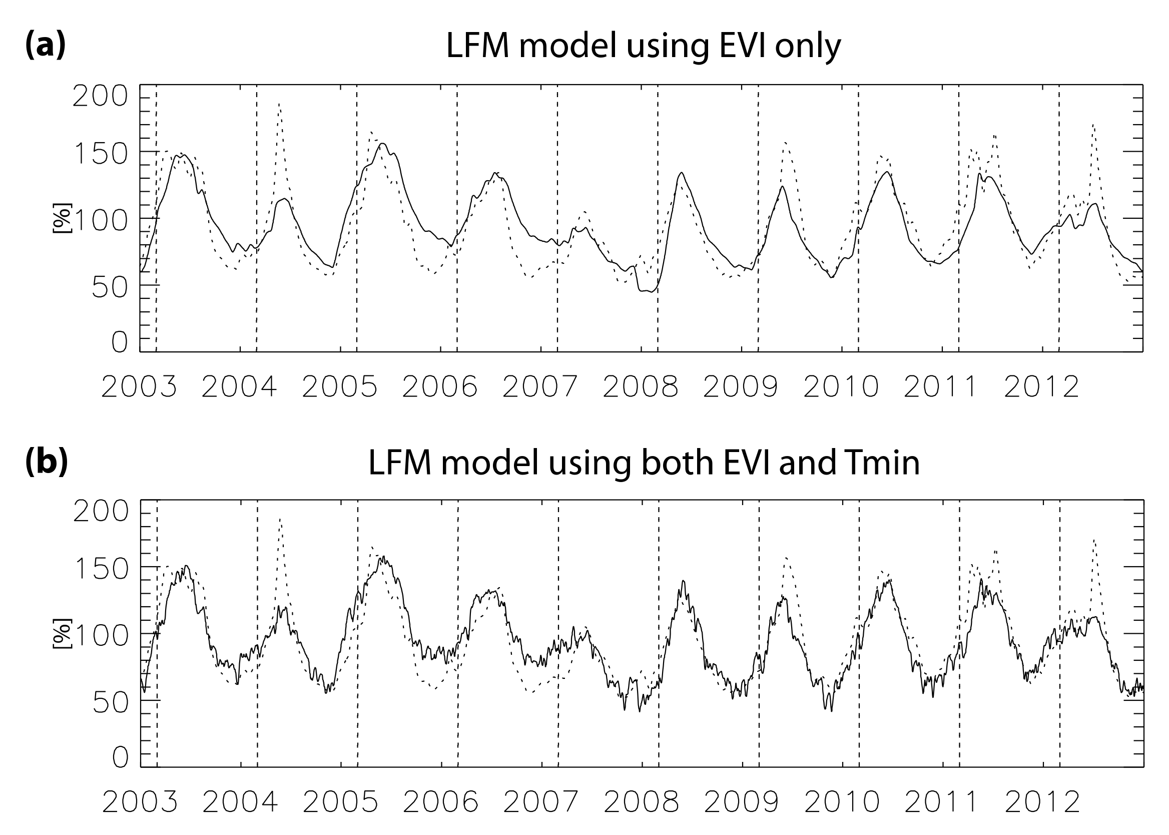
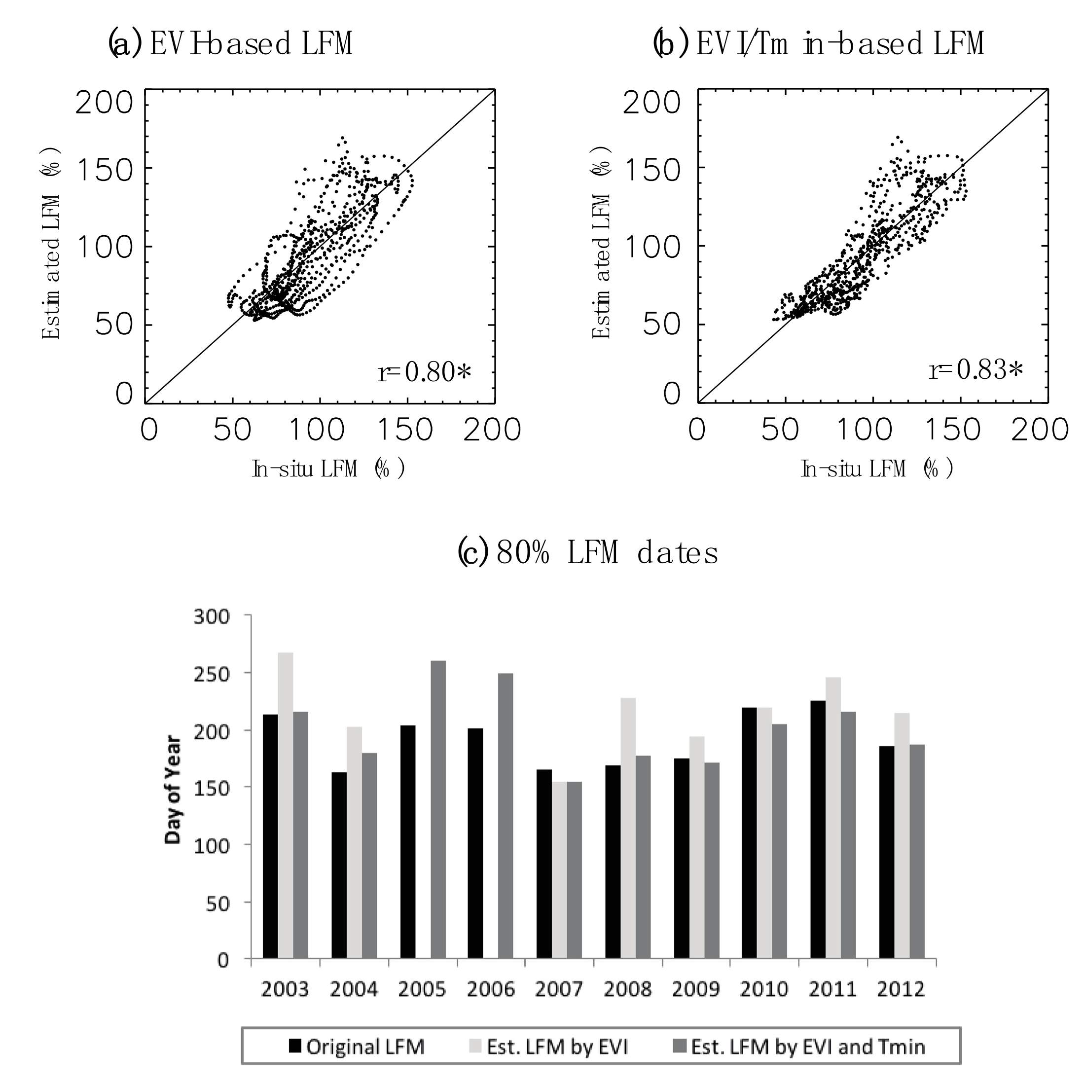
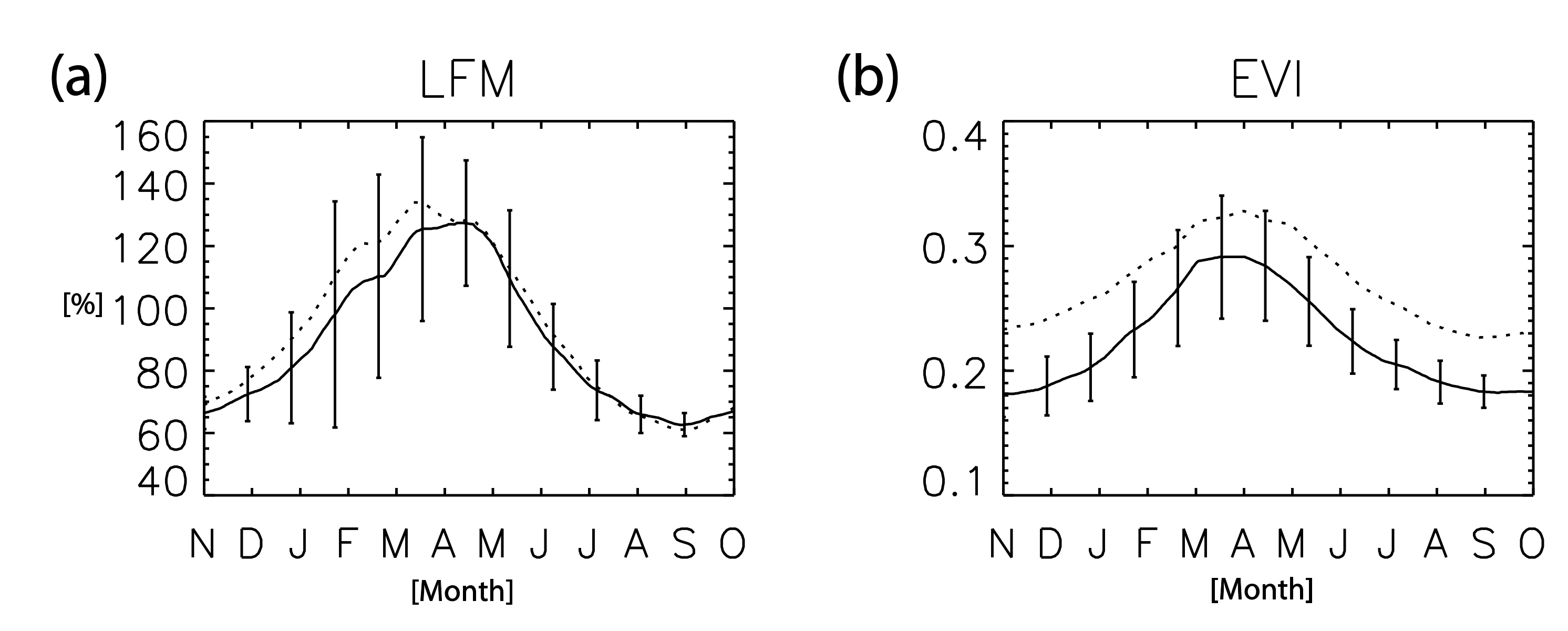
We have developed the EMF models based on the actual relationship with in-situ LFM, and evaluated the model performance with respect to the 10-year averages and interannual variability. The EVI-alone model showed a limited ability in estimating the timings and magnitudes of annual maxima and minima of LFM primarily because of consistently high in-situ LFM values, even in dry years for the maxima and the delayed response of EVI to precipitation when compared to LFM for the minima. However, seasonal variations, especially wet-to-dry trends of LFM (e.g., 90% LFM date in spring and early summer), were well estimated even on an interannual time scale. This result was consistent with the fact that vegetation greenness represented by EVI was also sensitive to environmental dryness [30]. The study here also found that the EMF model performance for low LFM values during summer and fall could be improved by including an air temperature variable as an additional predictor. This implies that excessive loss of moisture in vegetation on extremely hot days is better captured with the temperature parameter in addition to EVI.

While the 15-day running averaged data were utilized during our model development, a partial autocorrelation error might become non-negligible. We have investigated a transformation method using the Cochrane-Orcutt procedure to adjust the excessive correlation introduced by the temporal autocorrelation at lag 1 [31]. The transformed model showed some reduction in adjusted values of R². However, the outcome indicated a similar pattern as results of non-transformed model, thus the temporal autocorrelation will not affect the overall conclusion of this study.

The high correlation results of time-series data at different locations supported the significance of high-resolution satellite data in advancing the capability for fire danger assessment. This is because high-resolution satellite data would enable: (1) A selection of the appropriate vegetation type while eliminating irrelevant land-use classes (e.g., lakes, bare soil, urban areas, etc.); and, (2) an estimation of vegetation moisture condition over the vast extent where in-situ LFM measurements would not be extensively and frequently possible. Moreover, the correlations of time-series data between different locations, while characterizing the seasonal behavior consistently pertaining to the chaparral ecosystem, would not necessarily imply a homogenous spatial pattern of the vegetation conditions. 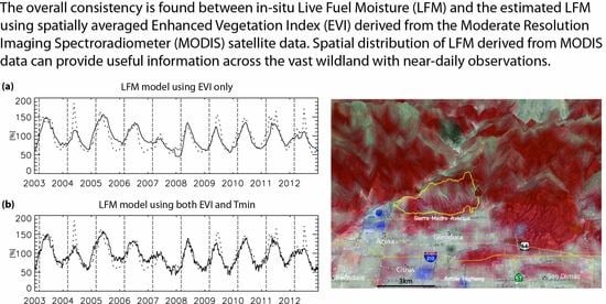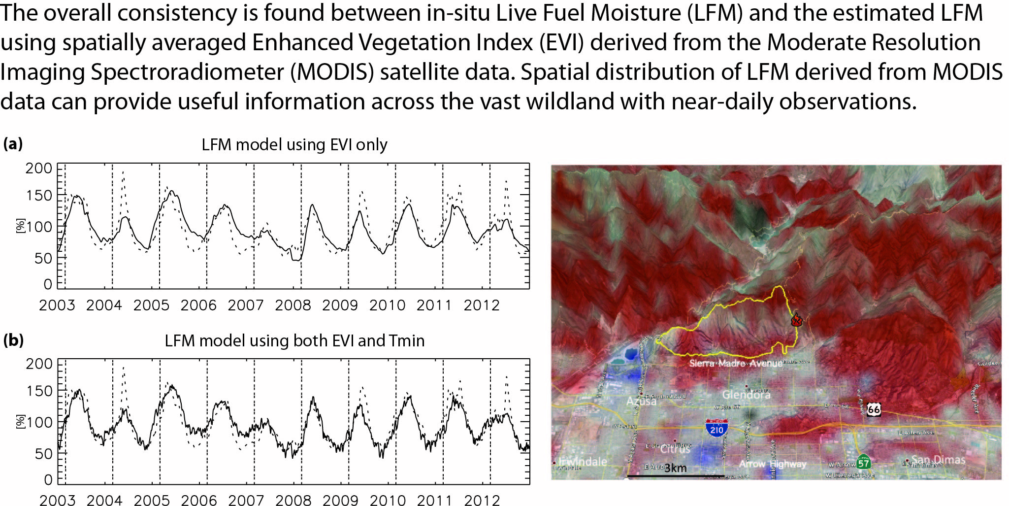In fact, as shown in Figure 8, the spatial distribution of LFM, as enabled by satellite observations, could be quite variable across the vast wildland. Such observations clearly and independently justified efforts by fire agencies to make LFM measurements at multiple sites critical to fire danger assessment. This result indicates that satellite-derived vegetation data could provide useful information in estimating vegetation moisture levels in SoCal after reducing multiple errors by spatial averaging, and also that in-situ LFM measurements were valid over a large extent beyond the intermediate vicinity of individual sampling sites.

5. Conclusions

The example of LFM map derived by the EMF shown in Figure 8 demonstrates the utility of satellite-based vegetation information for fire danger assessment with a high spatial resolution in SoCal. Such capability would improve more than one order of magnitude the current temporal and spatial coverage of the in-situ LFM measurement method conducted by fire agencies. The quality of such a kind of map could be further enhanced by LFM observations over the north-facing slopes and their modeling. Note that current LFM sampling sites were typically located in south-facing slopes, and thus the EMF model based on these data may be skewed towards the warmer and generally drier conditions that may result in an overestimation of fire risks. Therefore, LFM observations over the north-facing slopes and their modeling would be necessary for a more complete representation of LFM over complex terrain. Additional effective predictor(s), such as rainfall and soil moisture [32], should also be considered and tested for further improvement of the EMF model. Remotely sensed high-resolution soil moisture data, such as data from the Soil Moisture Active Passive (SMAP) mission [33], might provide additional information about regional soil moisture for synergistic enhancement of LFM estimation models.

There are uncertainties in both in-situ LFM and satellite VI data. First, a small sample size of the in-situ LFM may be insufficient for statistical analysis, resulting in large uncertainty. Weise et al. [5] reported that the uncertainty of LFM measurements varies significantly from ±20 to ±100%, depending on particular sites. Second, because of more intense insolation on the south sides of mountains, vegetation samples were only collected at south-facing mountain slopes; however, actual sample locations could change in different sampling excursions within an approximate three-acre lot selected by fire agencies where the topographic complexity might introduce more uncertainty. Regarding satellite data, VIs might have residual errors due to contaminations from clouds and aerosols that are not completely removed by the processing algorithms. Moreover, minor vegetation species might coexist within the chamise-dominant grid cells. There could be also uncertainties in the spatial coverage mismatch between LFM and VI data.

This study is only focused on the chaparral ecosystem in SoCal. However, the results can be applied to the Mediterranean region in Europe and elsewhere having similar climatic conditions via cross-validation process. In addition, our research framework can be adapted for applications to other wildfire-prone areas in the world with different climate conditions. Moreover, a universal model function approach should be considered in a future research, and such effort can be a key objective when sufficient statistical sampling across the extensive wildland and in-situ data records become sufficiently lengthened.

References

1. Syphard, A.D.; Radeloff, V.C.; Keeley, J.E.; Hawbaker, T.J.; Clayton, M.K.; Stewart, S.I.; Hammer, R.B. Human Influence on California Fire Regimes. Ecol. Appl. 2017, 17, 1388–1402. [Google Scholar] [CrossRef]
2. Mell, W.E.; Manzello, S.L.; Maranghides, A.; Butry, D.; Rehm, R.G. The wildland-urban interface fire problem—Current approaches and research needs. Int. J. Wildland Fire 2010, 19, 238–251. [Google Scholar] [CrossRef]
3. Deeming, J.E.; Burgan, R.E.; Cohen, J.D. The National Fire-Danger Rating System—1978; General Technical Report INT-169; U.S. Department of Agriculture, Forest Service, Intermountain Forest and Range Experiment Station: Ogden, UT, USA, 1977; p. 63. [Google Scholar]
4. Cohen, J.D.; Deeming, J.E. The National Fire-Danger Rating System: Basic Equations; General Technical Report GTR-PSW-82; USDA Forest Service, Pacific Southwest Forest and Range Experiment Station: Berkeley, CA, USA, 1985. [Google Scholar]
5. Weise, D.R.; Hartford, R.A.; Mahaffey, L. Assessing live fuel moisture for fire management applications. In Proceedings of the Fire in Ecosystem Management: Shifting the Paradigm from Suppression to Prescriptiontall Timbers Fire Ecology, Boise, ID, USA, 7–10 May 1998; Pruden, T.L., Brennan, L.A., Eds.; Tall Timbers Research Station: Tallahassee, FL, USA, 1988; Volume 20, pp. 49–55. [Google Scholar]
6. Countryman, C.M.; Dean, W.H. Measuring Moisture Content in Living Chaparral: A Field User’s Manual; General Technical Report PSW-36; USDA, Forest Service Pacific Southwest Forest and Range Experiment Station: Berkeley, CA, USA, 1979. [Google Scholar]
7. Dimitrakopoulos, A.; Papaioannou, K.K. Flammability assessment of Mediterranean forest fuels. Fire Technol. 2001, 37, 143–152. [Google Scholar] [CrossRef]
8. Chuvieco, E.; Cocero, D.; Riaño, D.; Martin, P.; Martínez-Vega, J.; de la Riva, J.; Pérez, F. Combining NDVI and surface temperature for the estimation of live fuel moisture content in forest fire danger rating. Remote Sens. Environ. 2004, 92, 322–331. [Google Scholar] [CrossRef]
9. Dennison, P.E.; Moritz, M.A.; Taylor, R.S. Examining predictive models of chamise critical live fuel moisture in the Santa Monica Mountains, California. Int. J. Wildland Fire 2008, 17, 18–27. [Google Scholar] [CrossRef]
10. Roberts, D.A.; Dennison, P.E.; Peterson, S.; Sweeney, S.; Rechel, J. Evaluation of Airborne Visible/Infrared Imaging Spectrometer (AVIRIS) and Moderate Resolution Imaging Spectrometer (MODIS) measures of live fuel moisture and fuel condition in a shrubland ecosystem in southern California. J. Geophys. Res. 2006, 111. [Google Scholar] [CrossRef]
11. Stow, D.; Niphadkar, M.; Kaiser, J. Time series of chaparral live fuel moisture maps derived from MODIS satellite data. Int. J. Wildland Fire 2006, 15, 347–360. [Google Scholar] [CrossRef]
12. Peterson, S.H.; Roberts, D.A.; Dennison, P.E. Mapping live fuel moisture with MODIS data: A multiple regression approach. Remote Sens. Environ. 2008, 112, 4272–4284. [Google Scholar] [CrossRef]
13. Dennison, P.E.; Roberts, D.A.; Peterson, S.H; Rechel, J. Use of Normalized Difference Water Index for monitoring live fuel moisture. Int. J. Remote Sens. 2005, 26, 1035–1042. [Google Scholar] [CrossRef]
14. Bowyer, P.; Danson, F.M. Sensitivity of spectral reflectance to variation in live fuel moisture content at leaf and canopy level. Remote Sens. Environ. 2004, 92, 297–308. [Google Scholar] [CrossRef]
15. Moran, M.S.; Vidal, A.; Troufleau, D.; Qi, J.; Clarke, T.R.; Pinter, P.J., Jr.; Mitchell, T.A.; Inoue, Y.; Neale, C.M.U. Combining multifrequency microwave and optical data for crop management. Remote Sens. Environ. 1997, 61, 96–109. [Google Scholar] [CrossRef]
16. Foley, J.A.; Prentice, I.C.; Ramankutty, N.; Levis, S.; Pollard, D.; Sitch, S.; Haxeltine, A. An integrated biosphere model of land surface processes, terrestrial carbon balance, and vegetation dynamics. Glob. Biogeochem. Cycles 1996, 10, 603–628. [Google Scholar] [CrossRef]
17. Myoung, B.; Choi, Y.S.; Hong, S.; Park, S.K. Inter- and intra-annual variability of vegetation in the Northern Hemisphere and its association with precursory meteorological factors. Glob. Biogeochem. Cycles 2013, 27, 31–42. [Google Scholar] [CrossRef]
18. Yebra, M.; Dennison, P.E.; Chuvieco, E.; Riaño, D.; Zylstra, P.; Hunt, E.R.; Danson, F.M.; Qi, Y.; Jurdao, S. A global review of remote sensing of live fuel moisture content for fire danger assessment: Moving towards operational products. Remote Sens. Environ. 2013, 136, 455–468. [Google Scholar] [CrossRef]
19. Wang, D.; Morton, D.; Masek, J.; Wu, A.; Nagol, J.; Xiong, X.; Levy, R.; Vermote, E.; Wolfe, R. Impact of sensor degradation on the MODIS NDVI time series. Remote Sens. Environ. 2012, 119, 55–61. [Google Scholar] [CrossRef]
20. Lyapustin, A.; Wang, Y.; Xiong, X.; Meister, G.; Platnick, S.; Levy, R.; Franz, B.; Korkin, S.; Hilker, T.; Tucker, J.; et al. Scientific impact of MODIS C5 calibration degradation and C6+ improvements. Atmos. Meas. Tech. 2014, 7, 4353–4365. [Google Scholar] [CrossRef]
21. Zhang, Y.; Song, C.; Band, L.E; Sun, G. Reanalysis of global terrestrial vegetation trends from MODIS products: Browning or greening? Remote Sens. Environ. 2017, 191, 145–155. [Google Scholar] [CrossRef]
22. Solano, R.; Didan, K.; Jacobson, A.; Huete, A. MODIS Vegetation Index User’s Guide; Vegetation Index and Phenology Lab, The University of Arizona: Tucson, AZ, USA, 2010. [Google Scholar]
23. Gitelson, A.A.; Kaufman, Y.J.; Stark, R.; Rundquist, D. Novel algorithms for remote estimation of vegetation fraction. Remote Sens. Environ. 2002, 80, 76–87. [Google Scholar] [CrossRef]
24. Serrano, L.; Ustin, S.L.; Roberts, D.A.; Gamon, J.A.; Penuelas, J. Deriving water content of chaparral vegetation from AVIRIS data. Remote Sens. Environ. 2000, 74, 570–581. [Google Scholar] [CrossRef]
25. Thenkabail, P.S.; Lyon, J.G.; Huete, A. Advances in Hyperspectral Remote Sensing of Vegetation and Agricultural Croplands. In Hyperspectral Remote Sensing of Vegetation, 1st ed.; Thenkabail, P.S., Lyon, J.G., Huete, A., Eds.; CRC Press: Boca Raton, FL, USA, 2011; ISBN 9781439845370. [Google Scholar]
26. InciWeb, Incidence Information System, Colby Fire. Available online: http://inciweb.nwcg.gov/incident/ 3766/ (accessed on 1 November 2017).
27. Dennison, P.E.; Moritz, M.A. Critical live fuel moisture in chaparral ecosystems: A threshold for fire activity and its relationship to antecedent precipitation. Int. J. Wildland Fire 2009, 18, 1021–1027. [Google Scholar] [CrossRef]
28. Wang, S.-Y.; Hipps, L.; Gillies, R.R.; Yoon, J.-H. Probable causes of the abnormal ridge accompanying the 2013–2014 California drought: ENSO precursor and anthropogenic warming footprint. Geophys. Res. Lett. 2014, 41, 3220–3226. [Google Scholar] [CrossRef]
29. Nghiem, S.V.; Neumann, G.; Kwan, J.; Chan, S.; Kafatos, M.; Myoung, B.; Hatzopoulos, N.; Kim, S.H.; Liu, X.; Calderon, S.; et al. Enhancing Wildland Fire Decision Support and Warning Systems; A NASA Project for Wildfire Applications Using Satellite Data, Final Report; Jet Propulsion Laboratory, California Institute of Technology: Pasadena, CA, USA, 2013. [Google Scholar]
30. Schnur, M.T.; Hongjie, X.; Wang, X. Estimating root zone soil moisture at distant sites using MODIS NDVI and EVI in a semi-arid region of southwestern USA. Ecol. Inform. 2010, 5, 400–409. [Google Scholar] [CrossRef]
31. Verbeek, M. A Guide to Modern Econometrics; John Wiley & Sons Ltd.: Hoboken, NJ, USA, 2004; ISBN 978-88-08-17054-5. [Google Scholar]
32. Qi, Y.; Dennison, P.E.; Spencer, J.; Riaño, D. Monitoring live fuel moisture using soil moisture and remote sensing proxies. Fire Ecol. 2012, 8, 71–87. [Google Scholar] [CrossRef]
33. Entekhabi, D.; Yueh, S.; O’Neill, P.E.; Kellogg, K.H.; Allen, A.; Bindlish, R.; Brown, M.; Chan, S.; Colliander, A.; Crow, W.T.; et al. SMAP Handbook, Soil Moisture Active Passive, Mapping Soil Moisture and Freeze/Thaw from Space; Jet Propulsion Laboratory, California Institute of Technology: Pasadena, CA, USA, 2014; 180p. [Google Scholar]
Figure 1. 16 live fuel moisture sampling sites overlaid on a Fire and Resource Assessment Program vegetation map. The colors indicate dominant vegetation species; only chamise-dominant areas (e.g., shrubland and scrubland) are shown. Two circles at La Tuna Canyon with a radius of 5 km and 10 km are also shown.
Remotesensing 10 00087 g001
Figure 2. A 10-year daily mean of (a) live fuel moisture and (b) enhanced vegetation index for the inland sites (solid line) and the coastal sites (dashed line). The x-axis represents months from November to October. Error bars are indicated by vertical bars for the inland sites only.
Remotesensing 10 00087 g002
Figure 3. 10-year time series (2003–2012) of live fuel moisture (a,c) and enhanced vegetation index (b,d) at the inland sites (a,b) and the coastal sites (c,d); The arrow in (a) indicates the period of live fuel moisture that was less than 75% in the 2011–2012 fire season.
Remotesensing 10 00087 g003
Figure 4. 10-year time series (November 2002–October 2012) of live fuel moisture (solid black) and enhanced vegetation index (dashed) with precipitation (solid gray) at (a) Bitter and (b) Schueren. The 15-day running mean is applied to each variable. Vertical dashed lines indicate beginning of each year.
Remotesensing 10 00087 g004
Figure 5. (a) Differences between minimum live fuel moisture and enhanced vegetation index dates for each year of the 10 years at Bitter (dark gray bar) and Schueren (light gray bar); (b) Same as (a) except differences between maximum dates.
Remotesensing 10 00087 g005
Figure 6. 10-year time series of (a) enhanced vegetation index (EVI)-estimated live fuel moisture (solid line) and in-situ live fuel moisture (dashed line) at Schueren; (b) is same as (a), except EVI and Tmin-estimated live fuel moisture (solid line).
Remotesensing 10 00087 g006
Figure 7. Daily time-scale scatter plots of the in-situ LFM in x-axis with (a) EVI-estimated LFM and (b) EVI and Tmin-estimated LFM in y-axis at Schueren; (c) Comparison of 80% LFM dates of in-situ LFM (black), EVI-estimated LFM (light gray), and EVI and Tmin-estimated LFM (dark gray) at Schueren. There were no values for the EVI-estimated LFM in 2006 and 2007 since EVI-alone estimated LFM values were higher than 80% the entire wet-dry season.
Remotesensing 10 00087 g007
Figure 8. The case of the Colby Fire in January 2014: Fuel dry-up map derived from MODIS data acquired on 8 January 2014 from the satellite Aqua over the San Gabriel Mountains, CA, USA. It clearly shows adjacent cities encroaching into surrounding wildland at multiple wildland-urban interfaces because of urbanization. Red represents severe dry-up due to a ~80% decrease in LFM from a level of 140% on 25 February 2013 resulting in an LFM below 60%, the critical fire danger threshold. The ignition location is marked with the flame symbol on the east side of the fire perimeter denoted by the yellow contours. Since the LFM color map is made translucent to see the landscape features, the accurate full color bar and true LFM map are shown in Figure S3 in the supporting information.
Remotesensing 10 00087 g008