Kinetic Analysis of the Color of Larch Sapwood and Heartwood during Heat Treatment

Abstract

The kinetics of color changes in larch sapwood and heartwood during heat treatment were investigated in this study in order to determine if the process of color change that occurs in the surface of wood can be regulated. Wood samples were heated at 90, 110, 130, and 150 °C in an oven, vacuum, and in an oven subjected to saturated steam for 3, 6, 9, and 12 h each. The results of the color measurement showed that the values of L* (lightness) and ΔE* (total color difference) decreased and increased in both the sapwood and heartwood, respectively, with increasing temperature and treatment time. The three kinetic model approach, consisting of (i) the time-temperature superposition principle (TTSP); (ii) zero-order reaction model; and, (iii) first-order reaction model, was used to model the kinetics of color changes. The results indicated that the L* value of the sample (including heartwood and sapwood) was well fitted to the first-order reaction model (R² = 0.9999). The Arrhenius activation energy was 14.2369 and 11.0984 kJ/mol for the sapwood and heartwood, respectively. The first-order reaction model also showed a better fit for the ΔE* values between sapwood and heartwood with higher R² values than the other two methods. Therefore, the color changes of larch wood could successfully be analyzed using the first-order reaction model.

1. Introduction

Wood color is one of the most important features of wood. Environmental factors (temperature, oxygen, moisture, and sunlight) and the impact of microorganisms are the main reasons for wood discoloration. It can be concluded from previous studies that the color of harvested wood is mainly related to the species [1], genetics [2], aging and weathering [3], drying process [4], the addition of wood preservatives, and chemical and thermal modification processes that are used in wood protection [5]. At present, heat treatment [6] has been widely used to modify harvested wood because it changes the color of wood and improves the apparent performance of wood [7]. Wood becomes darker, and the dimensional stability is improved after heat treatment [8,9,10]. The intrinsic reason for changes in wood color are mainly related to the chemical composition of wood, especially while taking into account its lignin and extractives [11,12]. The color evolution of heat treated wood is also related to the degradation of hemicelluloses [13] and the modification of the lignin polymer network [14]. Heat treatment results in the degradation of hemicelluloses and the oxidation of extractives in the wood, which produces substances (such as quinone) that cause the wood color to become more yellowish or reddish [15,16]. However, the color of wood became brown when being heated in the higher temperature (180–240 °C) is due to the condensation of polysaccharide by-products in the lignin molecule and the cleavage in β-O-4 [17,18,19,20].

Kinetics studies are generally used to study the color changes in fruits and vegetables, such as chestnuts [21], grapes [22], and rice [23]. The zero- or first-order reaction is suitable for most kinetic analyses, which are mostly applied in the food industry [24]. At a higher temperature, shorter time, and lower temperature over a longer period of time, the same mechanical relaxation phenomenon can be observed, which is referred to as the time-temperature superposition principle (TTSP). The TTSP was originally used to analyze material viscoelasticity [25], and it is widely used to analyze the mechanical properties of wood [26], such as wood creep performance [27,28,29]. The TTSP was also used in thermal degradation analysis combined with the Arrhenius equation, and it has been used for the determination of the color change of cellulose [30] and wood-plastic composite discoloration analysis [31]. In recent years, model-building methods have also been used in the field of wood thermal discoloration for further examination and experimentation. There has been an increasing number of different models created to study wood color trends during heat treatment [32,33,34]. In the study of wood thermal discoloration, the Arrhenius equation, while combined with the TTSP [35], is the most commonly used model to predict wood color change. However, the use of zero- and first-order reactions to model the color changes is relatively rare.

Dahurian larch (Larix gmelini) is the main species in the coniferous forest of the Greater Khingan Mountains, China [36]. It is rich in reserves, and it can be used for the raw materials that are necessary for housing construction, civil engineering, and the pole, boat, wood processing, and wood fiber industry. Of all coniferous wood, larch wood has excellent compression strength parallel to the grain and great static bending strength, and it has higher mechanical strength than pine trees. However, there is a clear difference in the color between the heartwood and sapwood of larch wood. The sapwood is light yellow in color, and the heartwood is brown to reddish-brown in color. In the drying process, the inconsistent color changes of sapwood and heartwood may result in uneven surface color of larch wood, which influences its utilization. The application of kinetics is mainly for the process control, like using the correlation between color parameters and heat-treatment intensity for quality control [7,37].

Most of the previous studies only used a method that modeled the color change. Few studies have created a better explanation for the contrast between these different models. The purpose of the current study is to use different heating methods to establish different models for the color change of larch wood, find the optimal kinetic model of larch wood color change, and provide a better theoretical basis for the drying process of larch wood. The color changes in wood drying process can be predicted as a function of time and temperature.

2. Materials and Methods

2.1. Selection and Preparation

Larch wood, aged 20 years, was harvested from northeast China in the Greater Khingan Mountains (E: 121°12′ to 127°00′, N: 50°10′ to 53°33′). A log that was 4 m in length was selected from the middle of the trees. The ratio of sapwood to heartwood was 5:1 with no existence of juvenile wood. The harvested log was 160–200 mm in diameter and 0.56 g/cm³ in basic density, with an initial moisture content of 70%. The log was debarked and cut into discs, with a thickness of 20 mm. The discs were sawed into 20 mm (longitudinal direction) × 50 mm (radial direction) × 20 mm (tangential direction) specimens (including the heartwood and sapwood). The moisture content of the samples was 27.85%, according to the weighing method. The samples were wrapped in plastic wrap and stored in a refrigerator (BCD-190TMPK, Haier refrigerator, Qingdao, Shandong, China) in order to prevent the evaporation of water.

2.2. Heat Treatment

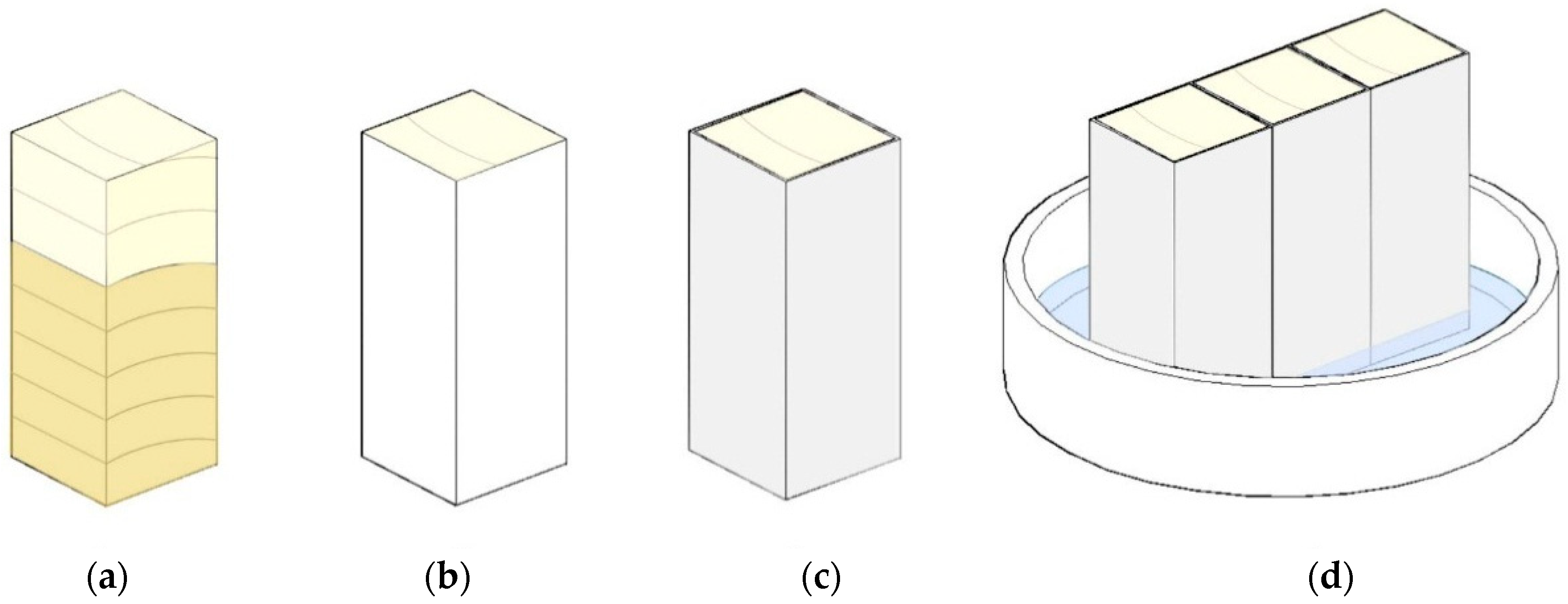
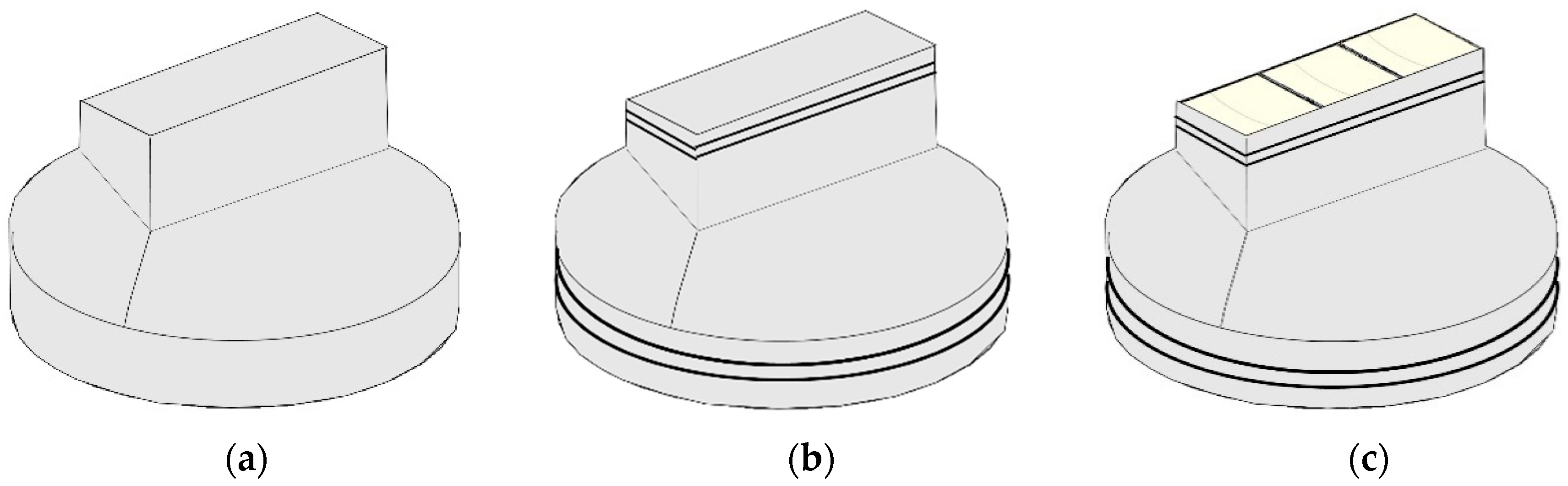
Samples without color defects, knots, and with apparent sapwood and heartwood were carefully selected (for a total of 120 samples). The pretreatment steps of the samples are shown in Figure 1. The sample was completely coated with silica gel and was wrapped with aluminum foil over an adhesive layer, and then the sample was placed in a Petri dish containing water, with the heartwood positioned so that it was in the water. The water in the Petri dish was continually replenished during the course of the experiment so that the dish never became dry. The equipment that was used to heat the wood in a vacuum was different from the equipment used to heat the wood in an oven and with saturated steam, in view of the low boiling point of water, and this is depicted in Figure 2. The vacuum device was obtained according to the following procedure: (1) the samples were wrapped in aluminum foil and placed in petri dishes, and they were held in place on the dish using a rubber band; (2) the aluminum foil was trimmed off the top of the specimen with a knife so that the dimensions of the aluminum foil were slightly smaller than the top of the wood and it snugly fit; and, (3) the three samples were tightened with a rubber band so that there was firm contact between the dish and the specimen.

The samples were heated in an oven at 90, 110, 130, and 150 °C for 3, 6, 9, and 12 h each. The thermal treatment temperatures in vacuum (0.08 MPa) were 90, 110, and in saturated steam were 130 °C, and 110 and 130 °C at the same treatment times. During the heating process, the water in the petri dish was maintained at all times, and a sample was taken every 3 h. All of the samples were removed after 12 h and were dried at atmospheric conditions to a moisture content of 12% for at least 15 days.

2.3. Color Measurement

The initial color parameters were measured for each sample using a Konica Minolta CM-2300d Chroma Meter (Konica Minolta Holdings, Inc., Tokyo, Japan), with a C standard illuminant and 8° standard observer, and simultaneous measurement of SCI (Specular Component Include) and SCE (Specular Component Exclude) was performed. The heated samples were cut into two parts along the center line of the radial direction, and then the color parameters inside the samples were measured. It performed three times of color test on six samples of each specimen. The color parameters L* (lightness), a* (green-red coordinate), and b* (blue-yellow coordinate) were measured for both the sample’s heartwood and sapwood. ΔL*, Δa*, Δb*, and ΔE* were calculated using the following Equations (1)–(4).

$$\Delta L^{*}=L_{heated}^{*}-L_{unheated}^{*}$$

(1)

$$\Delta a^{*}=a_{heated}^{*}-a_{unheated}^{*}$$

(2)

$$\Delta b^{*}=b_{heated}^{*}-b_{unheated}^{*}$$

(3)

$$\Delta E^{*}=\sqrt{{\left(\Delta L^{*}\right)}^2+{\left(\Delta a\right)}^2+{\left(\Delta b\right)}^2}$$

(4)

where ΔL*, Δa*, Δb*, and ΔE* represent the changes in the lightness, green/red coordinate, blue/yellow coordinate, and total color difference, respectively. The sapwood and heartwood of the samples were separately and repeatedly measured three times.

2.4. Kinetics Analysis

2.4.1. Arrhenius Equation and the Time-Temperature Superposition Principle

The temperature dependence chemical reaction rates of a substance can be expressed by the Arrhenius equation, according to Equation (5):

$$k=\mathrm{A}·\exp \left(-\frac{E_a}{RT}\right)$$

(5)

where k denotes the reaction rate constant, A denotes the frequency factor, E_a denotes the apparent activation energy, R denotes the gas constant, and T denotes the reaction absolute temperature. The calculation of E_a was obtained by the plot of ln (k)~1/T, according Equation (6).

$$\ln \left(k\right)=\ln \left(\mathrm{A}\right)-\frac{E_a}{RT}$$

(6)

The slope of the Arrhenius curve (ln (k)~1/T) is denoted by E_a. When the time-temperature equivalence principle (TTSP) is applied to the color change of wood, the same color change can be observed at short-term high temperatures and low temperatures for a long time. The behavior of increasing temperature is equivalent to prolonging the time. A smooth main curve can be obtained by moving the timeline and the color parameter axis. The shift distance of the time and color parameter axis is called the horizontal movement factor a_T (Equation (7)) and the vertical shift factor b_T (Equation (8)), respectively, as shown below:

$$a_T=\frac{t_T}{t_{ref}}$$

(7)

$$b_T=\frac{P_T}{P_{ref}}$$

(8)

where t_ref is the heat treatment time at a reference temperature T_ref, and t_T is the time that is required to give the same response at temperature T. P_T is the color parameter at T, and P_ref is the color parameter at T_ref. The calculation of a_T and b_T is based on the reference temperature of 130 °C.

2.4.2. Zero- and First-Order Reaction

The color changes in the wood surface are related to the reaction rate of the various chemical components within the wood. The equation representing the reaction rate is called the kinetic Equation (9):

$$\frac{dC}{dt}=-k{C}^n$$

(9)

where C denotes the quality factor (L*, a*, b*, and ΔE*); n denotes the reaction order; k denotes the reaction rate constant, h⁻¹; and, t denotes the reaction time, h.

In this study, zero order reactions (n = 0) and first order reactions (n = 1) were used. The kinetic equations are as follows:

$$\mathrm{zero}\mathrm{order}\mathrm{reaction}:kt=C_0-C$$

(10)

$$\mathrm{first}\mathrm{order}\mathrm{reaction}:kt=\mathrm{Ln}\left(C_0\right)-\mathrm{Ln}\left(C\right)$$

(11)

where C₀ denotes the initial quality factor.

2.5. Data Processing and Analysis

The mean values of L*, a*, b*, and ΔE* were calculated for each temperature and time after the data were obtained. The regression analysis of the data was carried out using Origin (Origin 8.5, OriginLab. Inc., Washington, DC, USA), Excel (Office 2013, Microsoft, Redmond, WA, USA), 1stOpt (1stOpt 1.5, 7D-Soft High Technology Inc., Beijing, China), and MATLAB (matlab2014a, MathWorks, Natick, MA, USA) software. A second-order polynomial was used to fit the data processed by the Arrhenius equation and the time-temperature superposition principle when using Matlab. The fitted degree of the experimental data and the model was measured using the coefficient of determination R² and the root mean square error RMSE as the standard. The values of R² that were closer to 1 indicated the better of the fitting model, and the smaller the RMSE, the higher the measurement accuracy.

3. Results and Discussion

3.1. The Color Change during Heat Treatment

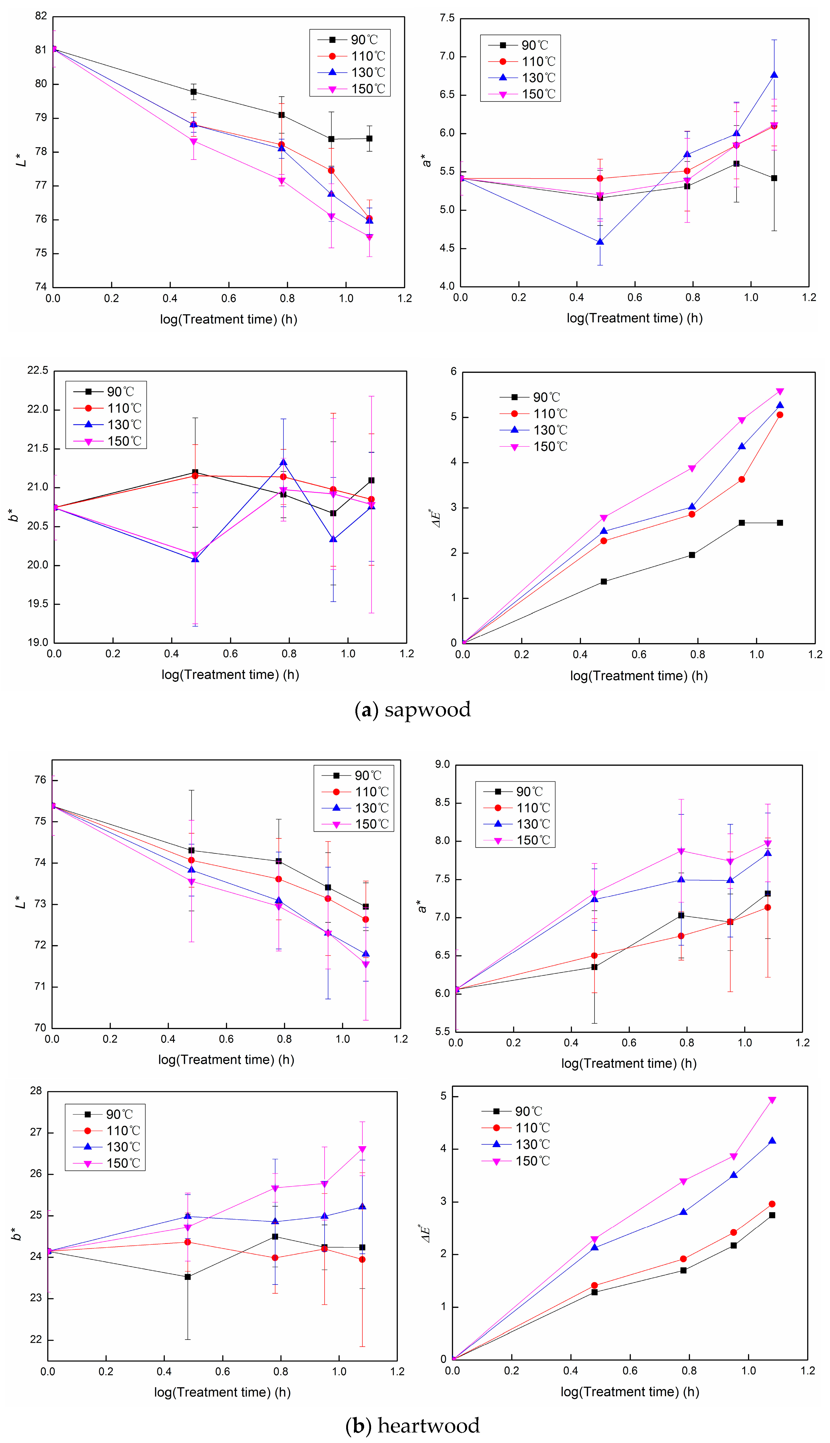
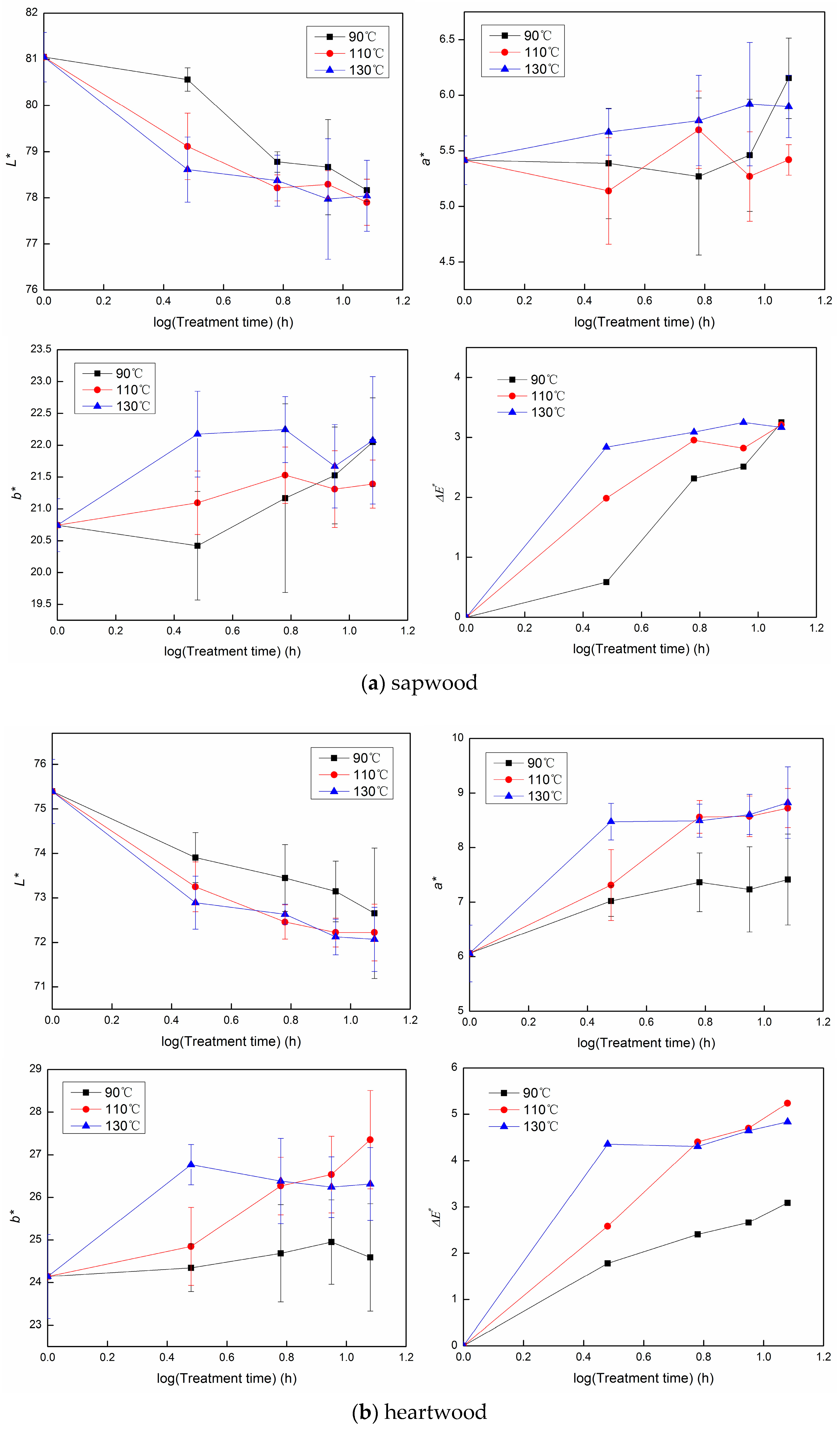
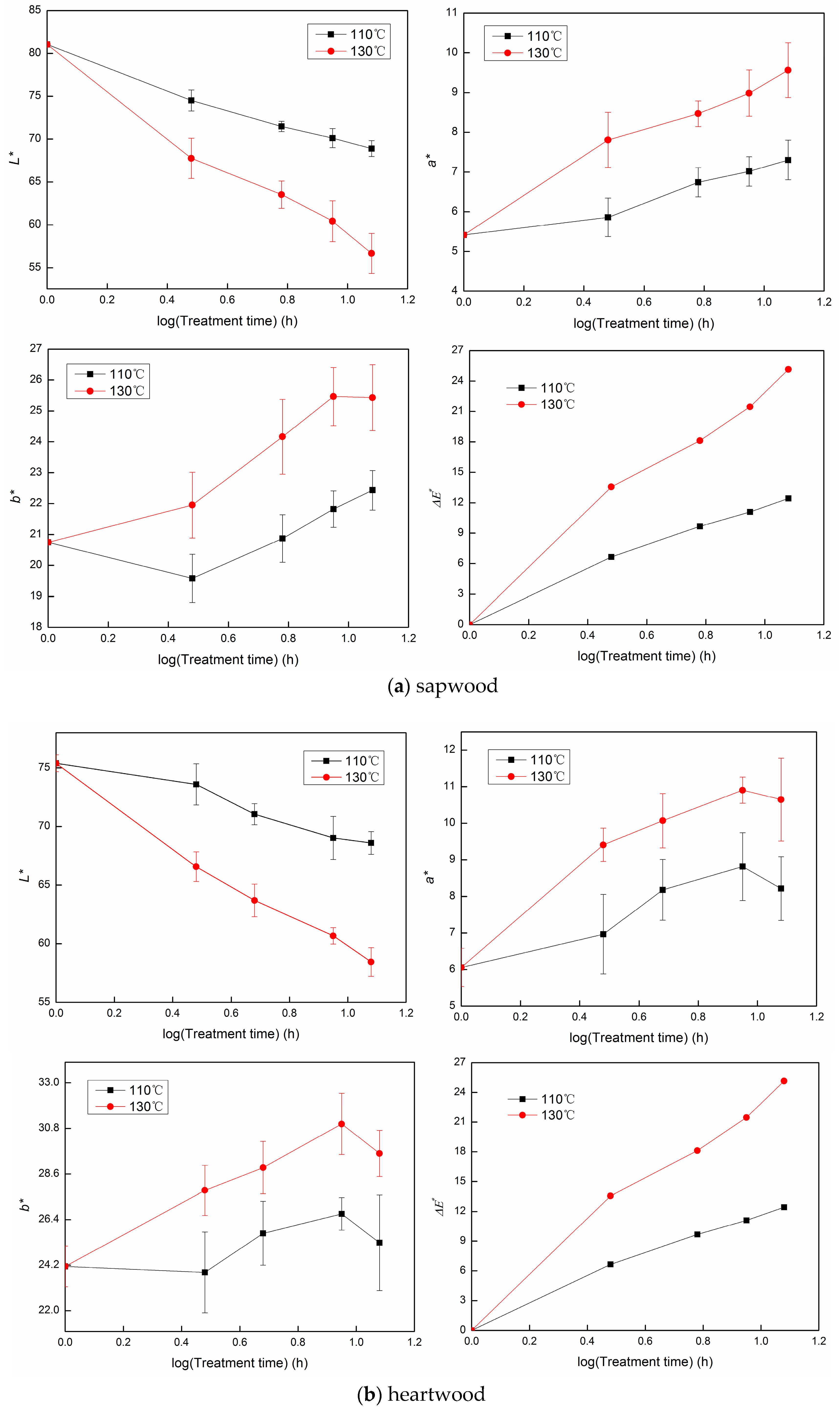
Figure 3, Figure 4 and Figure 5 show the L*, a*, b*, and ΔE* values of the sapwood and heartwood under different heating conditions. The surface color of the samples became darker after heat treatment. The brightness of the samples showed a decreasing trend with the increasing temperature and time, no matter the heat condition. These results have been verified by researchers such as Santos [38], W Ma [39] and Y Chen [8]. The changes in L* of the sapwood decreased from 81.05 to 56.68 when heated in saturated steam (130 °C/12 h), which in heartwood decreased from 75.39 to 58.45. The biggest changes occurred in saturated steam, which indicated that the chemical reaction was greatest in wood that received this treatment. The brightness of sapwood and heartwood was equal, at 68.88 and 68.59, respectively, when the samples were heated in saturated steam (110 °C/12 h). The a* and b* values increased overall after heat treatment, and these results differ from those of Sugi and Hiba [35]. The change trend of a* and b* values was different due to the different heat conditions and temperatures, suggesting that the changes in a* and b* were temperature dependent. The total color difference (ΔE*) increased with the increasing temperature and time, which was pronounced when wood was heated in saturated steam, as opposed to being heated in the oven and vacuum. The ΔE* in sapwood and heartwood increased from 0 to 25.16 and 18.38, respectively, when heated in saturated steam (130 °C/12 h). The changes in sapwood were significant when compared with heartwood, which may be due to the migration with water of the water-soluble extract in the heartwood to the sapwood. The result were also obtained in Araucaria angustifolia [40]. Monotone changes did not occur in the wood that was subject to a vacuum, which may be due to the evaporation of water in the petri dish that resulted in mutative vacuum conditions.

3.2. Kinetics Analysis

3.2.1. The Time-Temperature Superposition Principle (TTSP)

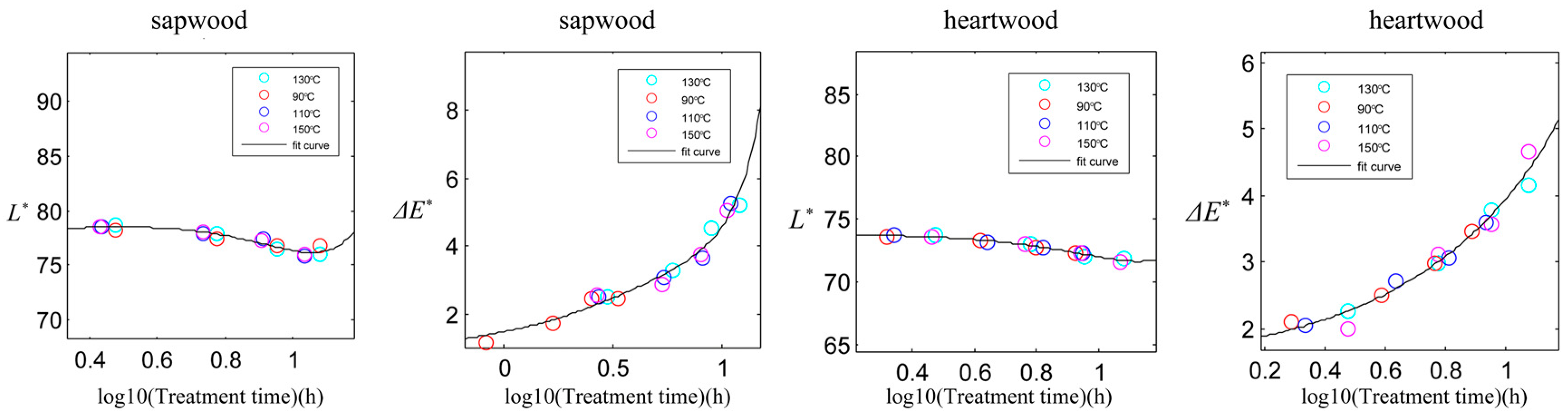
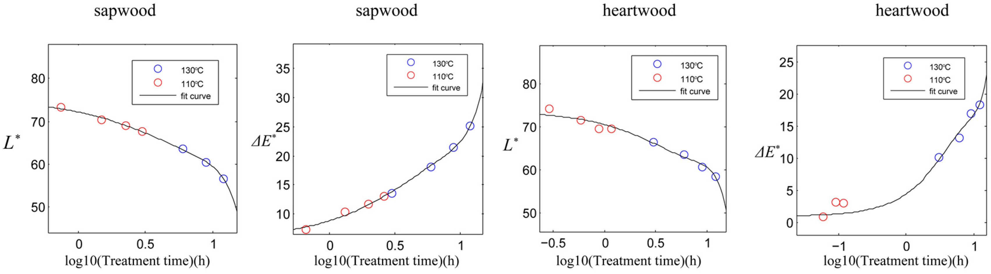
The changes in the L* and ΔE* values of the samples during the heat treatment were more regular, while the changes in a* and b* were relatively cluttered. Therefore, the kinetic analysis of this study was only for the L* and ΔE* of the samples. The smoothly fitted curves of the samples were obtained through the shift of the horizontal shift factor a_T and vertical shift factor b_T, which is shown in Figure 6, Figure 7 and Figure 8. Such a method has also been used to predict the color change during natural aging of Hinoki wood [41]. As shown in Figure 6, the fitted L* value decreased first and then slightly increased, which was different from the original change trend. However, the changes in the fitted ΔE* value for wood heated in an oven were similar to the original change trend. The fitted curve of L* and ΔE* for wood heated in a vacuum and saturated steam was the same as the previous trend (Figure 7 and Figure 8). Therefore, the TTSP method can be used to predict the color changes of samples.

Table 1. The coefficient of determination (R²) and root mean squared error (RMSE) of the samples under different heating conditions by time-temperature superposition principle (TTSP).

		Oven		Vacuum		Saturated Steam
		Sapwood	Heartwood	Sapwood	Heartwood	Sapwood	Heartwood
L*	R2	0.9987	0.9796	0.8180	0.9528	0.9972	0.9754
	RMSE	0.2769	0.2005	0.2989	0.0911	0.2735	0.8052
ΔE*	R2	0.9641	0.9717	0.8352	0.9108	0.9974	0.9575
	RMSE	0.2896	0.1884	0.3168	0.2351	0.2846	1.4888

summarizes the R² values for TTSP fitted to the data set at different heat conditions. The regression lines for the Arrhenius plot showed good linearity (R² > 0.822) for the hydrothermally treated wood in the treatment temperature range of 70–120 °C [35]. The R² value was less than 0.9 when the sapwood of the sample was heated in a vacuum, whereas the remaining samples were greater than 0.9. For the sapwood of the sample, the fitted result was R² (saturation steam) > R² (oven) > R² (vacuum), while the heartwood sample was R² (oven) > R² (saturation steam) > R² (vacuum). The fitted effect of the samples that were heated in the vacuum was the worst whether for the sapwood or heartwood. This indicated that the data set for wood treated in a vacuum was not suitable for TTSP. However, the fitted results of the samples under the remaining conditions were greater than 0.95, indicating that it is more optimal to use the TTSP to predict the color change of the samples when they are heated in an oven and are subjected to saturated steam.

3.2.2. Zero- and First-Order Reaction

The linear regression analysis was used with the L* and ΔE* values of the samples. The color parameters (L* and ΔE*) for the zero-order model are shown in

Table 2. The regression results from fitting the zero-order model to the L* value of the samples under different heating conditions.

		Oven				Vacuum			Saturated Steam
		90 °C	110 °C	130 °C	150 °C	90 °C	110 °C	130 °C	110 °C	130 °C
S 1	k	0.2638	0.4302	0.4595	0.5270	0.2635	0.3163	0.3226	1.1910	2.3079
	R2	0.8753	0.9317	0.9453	0.8892	0.9239	0.7514	0.6896	0.8304	0.8437
	RMSE	0.3781	0.4589	0.4450	0.7001	0.3605	0.6754	0.8533	1.9636	3.6164
H 2	k	0.2165	0.2513	0.3309	0.3473	0.2562	0.3354	0.3457	0.6308	1.6016
	R2	0.9458	0.9089	0.9384	0.9123	0.8454	0.7309	0.7127	0.9618	0.8724
	RMSE	0.2076	0.3040	0.3370	0.4133	0.3989	0.7600	0.8137	0.5262	2.2684

¹ sapwood ² heartwood.

and

Table 3. The regression results from fitting the zero-order model to the ΔE* value of the samples under different heating conditions.

		Oven				Vacuum			Saturated Steam
		90 °C	110 °C	130 °C	150 °C	90 °C	110 °C	130 °C	110 °C	130 °C
S 1	k	−0.1538	−0.3044	−0.3224	−0.3152	−0.2730	−0.1182	−0.0385	−0.6252	−1.2699
	R2	0.9298	0.9634	0.9794	0.9874	0.9218	0.8924	0.8894	0.9623	0.9958
	RMSE	0.1739	0.2172	0.1641	0.1228	0.3403	0.2318	0.1023	0.4538	0.2780
H 2	k	−0.1624	−0.1716	−0.2259	−0.2808	−0.1391	−0.2759	−0.0594	−0.5953	−0.9490
	R2	0.9942	0.9996	0.9998	0.9808	0.9754	0.9146	0.9113	0.9132	0.9757
	RMSE	0.0420	0.0106	0.0103	0.1372	0.0783	0.3763	0.0846	0.8263	0.5305

¹ sapwood ² heartwood.

, respectively, and the same parameters for the first-order kinetic model are shown in

Table 4. The regression results from fitting the first-order model to the L* value of the samples under different heating conditions.

		Oven				Vacuum			Saturated Steam
		90 °C	110 °C	130 °C	150 °C	90 °C	110 °C	130 °C	110 °C	130 °C
S 1	k	0.0033	0.0054	0.0058	0.0067	0.0033	0.0040	0.0067	0.0158	0.0331
	R2	0.9999	0.9999	0.9999	0.9999	0.9999	0.9999	0.9999	0.9999	0.9999
	RMSE	0.0047	0.0056	0.0054	0.0086	0.0045	0.0084	0.0107	0.0247	0.0448
H 2	k	0.0029	0.0034	0.0045	0.0047	0.0035	0.0045	0.0047	0.0087	0.0236
	R2	0.9999	0.9999	0.9999	0.9999	0.9999	0.9999	0.9999	0.9999	0.9999
	RMSE	0.0027	0.0040	0.0044	0.0054	0.0053	0.0102	0.0109	0.0071	0.0298

¹ sapwood ² heartwood.

and

Table 5. The regression results from fitting the first-order model to the ΔE* value of the samples under different heating conditions.

		Oven				Vacuum			Saturated Steam
		90 °C	110 °C	130 °C	150 °C	90 °C	110 °C	130 °C	110 °C	130 °C
S 1	k	−0.0771	−0.0881	−0.0873	−0.0775	−0.1742	−0.0466	−0.0127	−0.0671	−0.0674
	R2	0.9762	0.9994	0.9988	0.9988	0.9269	0.9739	0.9814	0.9990	0.9999
	RMSE	0.0941	0.0272	0.0384	0.0525	0.3246	0.0961	0.0337	0.0693	0.0349
H 2	k	−0.9844	−0.0818	−0.0744	−0.0810	−0.0584	−0.0730	−0.0129	−0.1391	−0.0679
	R2	0.9996	0.9979	0.9988	0.9967	0.9907	0.9886	0.9941	0.9906	0.9998
	RMSE	0.0110	0.0264	0.0262	0.0556	00471	0.1207	0.0188	0.2352	0.0497

¹ sapwood ² heartwood.

, respectively.

It can be seen from Table 2 and Table 4 that the k value from fitting the zero-order and first-order model to the L* value increased with the increasing temperature. The reaction rate constant (k) for wood heated in saturated steam was significantly larger than that obtained for the other two heating methods, indicating that the temperature and heating conditions have a great effect on the reaction rate of the samples. The larger the value of k, the greater the chemical reaction that occurred in the samples, and the greater the corresponding color change, which indicates that the color change that occurred in the wood that was subjected to saturated steam was largest. The k value from fitting the zero-order and first-order model to the ΔE* value was irregular when compared with the L* value, which may have occurred because of the existence of a* and b*.

R² reflects the precision of the data set to the fitted model. The larger the R² value and the lower the value of RMSE, the better the fit degree of the samples. When the zero-order reaction model was used to analyze the L* value of the samples (Table 2), the regression result R² for the sapwood was between 0.68 and 0.94, and the heartwood was 0.71 < R² < 0.96. The RMSE value of the zero-order model with that of TTSP (Table 1) were almost the same. When the ΔE* value was fitted (Table 3), the result for sapwood was 0.87 < R² < 0.99, and the heartwood was 0.91 < R² < 0.99. The R² value fitted to ΔE* was higher than L* in general, which demonstrated that the fitted degree of the zero-order model for the L* value was better than ΔE*.

The R² value of the samples was 0.9999 (Table 4) when the first-order reaction model was used to fit the L* values for linear regression, and the value of RMSE (RMSE < 0.1) was lower than TTSP and zero-order model, which illustrated that the use of the first-order reaction model for L* was very good. The R² value of the first-order model for ΔE* values (Table 5) was lower than the L* value, and the majority of wood samples were larger than 0.99, except for the data for the wood heated in vacuum.

When compared with the above four tables, it can be concluded that the R² (0.9999) for the first-order reaction model was greater than the R² value (R² < 0.99) for the zero-order reaction model when the L* value was fitted; the R² value for the zero-order model for the ΔE* value was lower than the R² for the first-order reaction model. Therefore, when compared with the zero-order reaction model, the first-order reaction model (RMSE < 0.1) was more favorable to correctly model the color changes of the samples.

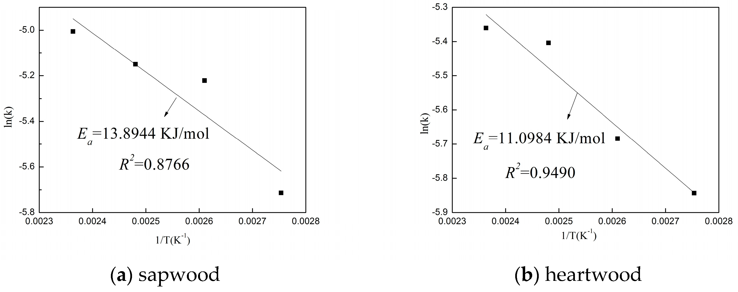
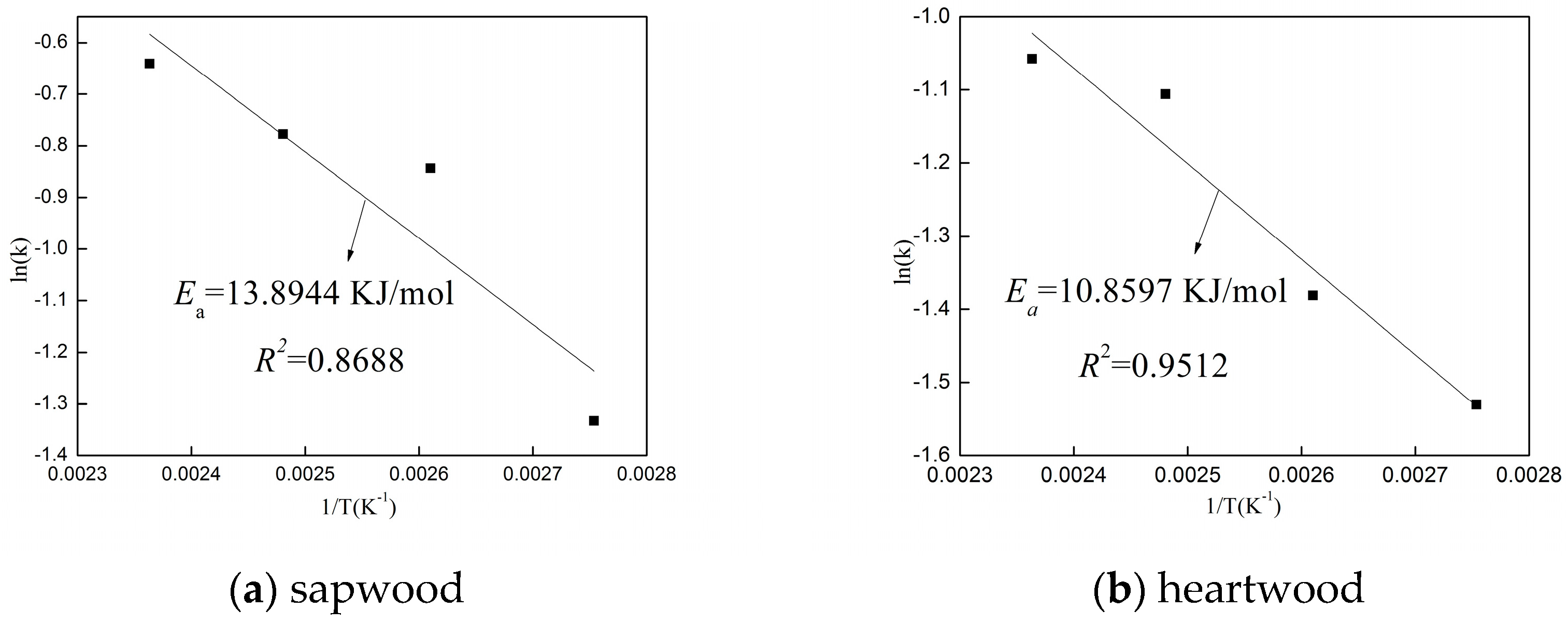
The apparent activation energy (Figure 9 and Figure 10) for change in L* of the sapwood and heartwood was calculated by the Arrhenius curve on the basis of the zero-order reaction and the first-order reaction. The E_a calculated by the zero-order model for the changes in L* of the sapwood and heartwood was 13.89 kJ/mol and 10.8597 kJ/mol, respectively, which was 14.2359 kJ/mol (sapwood) and 11.0984 kJ/mol (heartwood) by the first-order reaction. Both of the E_a values are lower than keyaki wood [33] and Hinokiwood [32]. The R² for the first-order reaction was greater than the zero-order reaction, which corresponded to the previous fitness result, and indicated that the first-order reaction can better express the apparent activation energy of the sample. The E_a of the sapwood was higher than that of the heartwood and it corresponded to the change in the k value between the sapwood and heartwood. The difference in apparent activation energy between the sapwood and heartwood may be related to distinct chemical components [33]. The E_a value calculated by the first-order model was higher than that of the zero-order model, indicating that the reactivity of the chemical composition in the sample represented by the first-order reaction was greater than the reactivity that was represented by the zero-order reaction.

3.2.3. The comparison of the Three Fitting Models

Table 6. The comparison of R² values after the fitting of the L* value using three kinetic models.

	TTSP	Zero-Order Reaction	First-Order Reaction
Sapwood	0.8180 < R2 < 0.9987	0.6896 < R2 < 0.9453	0.9999
Heartwood	0.9528 < R2 < 0.9796	0.7127 < R2 < 0.9618	0.9999

and

Table 7. The comparison of R² values after the fitting of the ΔE* value using three kinetic models.

	TTSP	Zero-Order Reaction	First-Order Reaction
Sapwood	0.8352 < R2 < 0.9974	0.8724 < R2 < 0.9958	0.9269 < R2 < 0.9999
Heartwood	0.9108 < R2 < 0.9717	0.9113 < R2 < 0.9998	0.9886 < R2 < 0.9998

summarize the R² of three kinetic models. In Table 6, the R² value for the L* value of the sapwood and heartwood fitted by the first-order models was highest and the zero-order model was the lowest. The R² for the ΔE* was still largest when compared with other methods, while for the TTSP, it was the worst (Table 7). Therefore, the first-order model was the best model for predicting the color change of sapwood and heartwood.

4. Conclusions

In this study, larch wood samples were heated in an oven (90, 110, 130, and 150 °C), vacuum (90, 110, and 130 °C), and under saturated steam (110 and 130 °C) for 3, 6, 9, and 12 h each. The color of all the samples was deepened after heat treatment. The color change of sapwood was greater than that of heartwood. The L* value decreased and the ΔE* value increased with increasing temperature and time. The changes in a* and b* were temperature dependent and varied in the sapwood and heartwood. The largest changes in L* and ΔE* occurred when wood was heated in saturated steam, and the smallest changes occurred in a vacuum. This may be due to the presence of moisture and oxygen during the heating process, which accelerated the chemical reaction within the samples.

Three types of kinetic models (TTSP, zero-order, and first-order model) were used to analyze the color change. The R² value for the L* value (R² = 0.9999) and ΔE* (R² > 0.92) of the sapwood and heartwood fitted by the first-order models was the highest. The E_a calculated by the first-order model for change in L* of the sapwood and heartwood was 14.2359 kJ/mol and 11.0984 kJ/mol, respectively. The results signified that the first-order model successfully modeled the color change of the samples. The results of this study can provide predictions for the color change of wood that occurs during the heat treatment process and can serve as a reference for the drying process and color control.

References

- Pâques, L.E.; García-Casas, M.D.C.; Charpentier, J.P. Distribution of heartwood extractives in hybrid larches and in their related European and Japanese larch parents: Relationship with wood colour parameters. Eur. J. For. Res. 2013, 132, 61–69. [Google Scholar] [CrossRef]
- Montes, C.S.; Hernández, R.E.; Beaulieu, J.; Weber, J.C. Genetic variation in wood color and its correlations with tree growth and wood density of Calycophyllum spruceanum at an early age in the Peruvian Amazon. New For. 2008, 35, 57–73. [Google Scholar] [CrossRef]
- Moya, R.; Berrocal, A. Wood colour variation in sapwood and heartwood of young trees of Tectona grandis and its relationship with plantation characteristics, site, and decay resistance. Ann. For. Sci. 2010, 67, 109. [Google Scholar] [CrossRef]
- Aguilartovar, D.; Moya, R.; Tenorio, C. Wood color variation in undried and kiln-dried plantation-grown lumber of Vochysia guatemalensis. Maderas Ciencia Y Tecnología 2009, 11, 207–216. [Google Scholar]
- Johansson, D.; Morén, T. The potential of colour measurement for strength prediction of thermally treated wood. Holz als Roh-und Werkstoff 2006, 64, 104–110. [Google Scholar] [CrossRef]
- Kubovský, I.; Kačík, F. Colour and chemical changes of the lime wood surface due to CO2 laser thermal modification. Appl. Surf. Sci. 2014, 321, 261–267. [Google Scholar] [CrossRef]
- Brischke, C.; Welzbacher, C.R.; Brandt, K.; Rapp, A.O. Quality control of thermally modified timber: Interrelationship between heat treatment intensities and CIE l*a*b* color data on homogenized wood samples. Holzforschung 2007, 48, 17–22. [Google Scholar] [CrossRef]
- Chen, Y.; Fan, Y.; Gao, J.; Stark, N.M. The effect of heat treatment on the chemical and color change of black locust (Robinia pseudoacacia) wood flour. Bioresources 2012, 7, 1157–1170. [Google Scholar] [CrossRef]
- Zanuncio, A.J.V.; Carvalho, A.G.; Souza, M.T.D.; Jardim, C.M.; Carneiro, A.D.C.O.; Colodette, J.L. Effect of extractives on wood color of heat treated Pinus radiata and Eucalyptus pellita. Maderas Ciencia Y Tecnologia 2015, 17, 857–864. [Google Scholar] [CrossRef]
- Tuong, V.M.; Li, J. Effect of heat treatment on the change in color. BioResources 2010, 5, 1257–1267. [Google Scholar]
- Sundqvist, B.; Morén, T. The influence of wood polymers and extractives on wood colour induced by hydrothermal treatment. Holz als Roh-und Werkstoff 2002, 60, 375–376. [Google Scholar] [CrossRef]
- Wei, Y.; Wang, M.; Zhang, P.; Chen, Y.; Gao, J.; Fan, Y. The role of phenolic extractives in color changes of locust wood (Robinia pseudoacacia) during heat treatment. BioResources 2017, 12, 7041–7055. [Google Scholar]
- Tjeerdsma, B.F.; Militz, H. Chemical changes in hydrothermal treated wood: Ftir analysis of combined hydrothermal and dry heat-treated wood. Eur. J. Wood Wood Prod. 2005, 63, 102–111. [Google Scholar] [CrossRef]
- Brosse, N.; Hage, R.E.; Chaouch, M.; Pétrissans, M.; Dumarçay, S.; Gérardin, P. Investigation of the chemical modifications of beech wood lignin during heat treatment. Polym. Degrad. Stab. 2010, 95, 1721–1726. [Google Scholar] [CrossRef]
- Chen, Y.; Gao, J.; Fan, Y.; Tshabalala, M.A.; Stark, N.M. Heat-induced chemical and color changes of extractive-free black locust (Robinia pseudoacacia) wood. Bioresources 2012, 7, 2236–2248. [Google Scholar] [CrossRef]
- Chen, Y.; Fan, Y.; Gao, J.; Tshabalala, M.A.; Stark, N.M. Spectroscopic analysis of the role of extractives on heat-induced discoloration of black locust (Robinia pseudoacacia). Wood Mater. Sci. Eng. 2012, 7, 209–216. [Google Scholar] [CrossRef]
- Srinivas, K.; Pandey, K.K. Effect of heat treatment on color changes, dimensional stability, and mechanical properties of wood. J. Wood Chem. Technol. 2012, 32, 304–316. [Google Scholar] [CrossRef]
- Windeisen, E.; Strobel, C.; Wegener, G. Chemical changes during the production of thermo-treated beech wood. Wood Sci. Technol. 2007, 41, 523–536. [Google Scholar] [CrossRef]
- Kačíková, D.; Kačík, F.; Cabalová, I.; Durkovič, J. Effects of thermal treatment on chemical, mechanical and colour traits in Norway spruce wood. Bioresour. Technol. 2013, 144, 669–674. [Google Scholar] [CrossRef] [PubMed]
- González-Peña, M.M.; Curling, S.F.; Hale, M.D. On the effect of heat on the chemical composition and dimensions of thermally-modified wood. Polym. Degrad. Stab. 2009, 94, 2184–2193. [Google Scholar] [CrossRef]
- Lixia, H.; Bo, L.; Shaojin, W. Kinetics of color degradation of chestnut kernel during thermal treatment and storage. Int. J. Agric. Biol. Eng. 2015, 8, 106–115. [Google Scholar] [CrossRef]
- Dong, Y.H.; Zhang, R.Y.; Zhang, Z.T.; Yang, L.W.; Xue, C.H.; Wei, J.; Yang, R.Y. Study on kinetics of color changes in thompson seedless grapes during drying process. Adv. Mater. Res. 2013, 726, 456–462. [Google Scholar] [CrossRef]
- Devi, M.K.; Das, S.K. Kinetics of color changes of popped rice during microwave popping: Effect of salt and moisture content. J. Food Process Eng. 2017, 40, e12560. [Google Scholar] [CrossRef]
- Pathare, P.B.; Opara, U.L.; Al-Said, F.A.-J. Colour measurement and analysis in fresh and processed foods: A review. Food Bioprocess Technol. 2013, 6, 36–60. [Google Scholar] [CrossRef]
- Gross, B. Time-temperature superposition principle in relaxation theory. J. Appl. Phys. 1969, 40, 3397. [Google Scholar] [CrossRef]
- Nakano, T. Applicability condition of time-temperature superposition principle (TTSP) to a multi-phase system. Mech. Time-Depend. Mater. 2013, 17, 439–447. [Google Scholar] [CrossRef] [Green Version]
- Peng, H.; Jiang, J.; Lu, J.; Cao, J. Application of time-temperature superposition principle to chinese fir orthotropic creep. J. Wood Sci. 2017, 63, 455–463. [Google Scholar] [CrossRef]
- Wang, F.; Huang, T.; Shao, Z. Application of ttsp to wood-development of a vertical shift factor. Holzforschung 2017, 71, 51–55. [Google Scholar] [CrossRef]
- Jabbar, A.; Militký, J.; Kale, B.M.; Rwawiire, S.; Nawab, Y.; Baheti, V. Modeling and analysis of the creep behavior of jute/green epoxy composites incorporated with chemically treated pulverized nano/micro jute fibers. Ind. Crops Prod. 2016, 84, 230–240. [Google Scholar] [CrossRef]
- Matsuo, M.; Umemura, K.; Kawai, S. Kinetic analysis of color changes in cellulose during heat treatment. J. Wood Sci. 2012, 58, 113–119. [Google Scholar] [CrossRef] [Green Version]
- Xu, C.; Xing, C.; Pan, H.; Kamdem, P.D.; Matuana, L.M.; Jian, W.; Wang, G. Time-temperature superposition principle application to the hygrothermal discoloration of colored high-density polypropylene/wood composites. Polym. Compos. 2016, 37, 1016–1020. [Google Scholar] [CrossRef]
- Matsuo, M.; Yokoyama, M.; Umemura, K.; Gril, J.; Yano, K.I.; Kawai, S. Color changes in wood during heating: Kinetic analysis by applying a time-temperature superposition method. Appl. Phys. A 2010, 99, 47–52. [Google Scholar] [CrossRef] [Green Version]
- Matsuo, M.; Umemura, K.; Kawai, S. Kinetic analysis of color changes in keyaki (zelkova serrata) and sugi (Cryptomeria japonica) wood during heat treatment. J. Wood Sci. 2014, 60, 12–20. [Google Scholar] [CrossRef]
- Inagaki, T.; Matsuo, M.; Tsuchikawa, S. Nir spectral–kinetic analysis for thermally degraded sugi (Cryptomeria japonica) wood. Appl. Phys. A 2016, 122, 208. [Google Scholar] [CrossRef]
- Matsuo, M.U.; Mitsui, K.; Kobayashi, I.; Kohara, M.; Yoshida, M.; Yamamoto, H. Effect of hygrothermal treatment on wood properties: Color changes and kinetic analysis using four softwood and seven hardwood species. Wood Sci. Technol. 2016, 50, 1145–1160. [Google Scholar] [CrossRef]
- Hu, T.; Sun, L.; Hu, H.; Weise, D.R.; Guo, F. Soil respiration of the dahurian larch (Larix gmelinii) forest and the response to fire disturbance in Da Xing’an Mountains, China. Sci. Rep. 2017, 7, 2967. [Google Scholar] [CrossRef] [PubMed]
- Robert Welzbacher, C.; Brischke, C.; Otto Rapp, A. Influence of treatment temperature and duration on selected biological, mechanical, physical and optical properties of thermally modified timber. Wood Mater. Sci. Eng. 2007, 2, 66–76. [Google Scholar] [CrossRef]
- Santos, D.V.B.D.; Moura, L.F.D.; Brito, J.O. Effect of heat treatment on color, weight loss, specific gravity and equilibrium moisture content of two low market valued tropical woods. Wood Res. 2014, 59, 253–264. [Google Scholar]
- Ma, W.; Qiang, T.; Guo, M. Effect of high temperature heat treatment on color change of imitate precious wood of larch. J. Northeast For. Univ. 2016, 44, 37–41. [Google Scholar]
- Oliveira, R.M.D.; Brisolari, A.; Sales, A.; Gonçalves, D. Wettability, shrinkage and color changes of Araucaria angustifolia after heating treatment. Mater. Res. 2010, 13, 351–354. [Google Scholar] [CrossRef]
- Matsuo, M.; Yokoyama, M.; Umemura, K.; Sugiyama, J.; Kawai, S.; Gril, J.; Kubodera, S.; Mitsutani, T.; Ozaki, H.; Sakamoto, M. Aging of wood: Analysis of color changes during natural aging and heat treatment. Holzforschung 2011, 65, 361–368. [Google Scholar] [CrossRef] [Green Version]
Figure 1.
The preprocessing of samples heated in an oven and subjected to saturated steam. (a) Original wood sample (including heartwood and sapwood); (b) the wood sample was coated on the outer surface with silica gel and the bottoms of the wood blocks were left open to the air, matching the tops (the white part in Figure 1b); (c) the wood sample was wrapped in aluminum foil (the silver part in Figure 1c) over an adhesive layer; and, (d) the treated heartwood sample was placed in a Petri dish containing water.
Figure 2.
The preprocessing of a sample heated in vacuum. (a) The sample were wrapped in aluminum foil and placed in petri dishes; (b) a rubber band was used to hold the samples in place on the dish; and, (c) the aluminum foil was trimmed off the top with a knife.
Figure 3.
The L*, a*, b*, and ΔE* values of the samples that were heated in an oven.
Figure 4.
The L*, a*, b*, and ΔE* values of the samples that were heated in a vacuum.
Figure 5.
The L*, a*, b*, and ΔE* values of the samples that were heated in saturated steam.
Figure 6.
The fitting model using horizontal shift factor aT and vertical shift factor bT for L* and ΔE* when samples were heated in an oven.
Figure 7.
The fitting model using horizontal shift factor aT and vertical shift factor bT for L* and ΔE* when samples were heated in a vacuum.
Figure 8.
The fitting model using horizontal shift factor aT and vertical shift factor bT for L* and ΔE* when samples were heated in saturated steam.
Figure 9.
Arrhenius plots for L* of samples in zero-order reaction, and calculated apparent activation energy (Ea).
Figure 10.
Arrhenius plots for L* of samples in first-order reaction, and calculated apparent activation energy (Ea).