


A Comparative Study of Deep-Learning Autoencoders (DLAEs) for Vibration Anomaly Detection in Manufacturing Equipment


Department of Aeronautics, Mechanical and Electronic Convergence Engineering, Kumoh National Institute of Technology, 61 Daehak-ro, Gumi-si 39177, Republic of Korea
*
Author to whom correspondence should be addressed.
Electronics 2024, 13(9), 1700; https://doi.org/10.3390/electronics13091700
Submission received: 28 March 2024
/
Revised: 15 April 2024
/
Accepted: 26 April 2024
/
Published: 27 April 2024
(This article belongs to the Special Issue Current Trends on Data Management)
Abstract
:Speed reducers (SR) and electric motors are crucial in modern manufacturing, especially within adhesive coating equipment. The electric motor mainly transforms electrical power into mechanical force to propel most machinery. Conversely, speed reducers are vital elements that control the speed and torque of rotating machinery, ensuring optimal performance and efficiency. Interestingly, variations in chamber temperatures of adhesive coating machines and the use of specific adhesives can lead to defects in chains and jigs, causing possible breakdowns in the speed reducer and its surrounding components. This study introduces novel deep-learning autoencoder models to enhance production efficiency by presenting a comparative assessment for anomaly detection that would enable precise and predictive insights by modeling complex temporal relationships in the vibration data. The data acquisition framework facilitated adherence to data governance principles by maintaining data quality and consistency, data storage and processing operations, and aligning with data management standards. The study here would capture the attention of practitioners involved in data-centric processes, industrial engineering, and advanced manufacturing techniques.
1. Introduction
The manufacturing industry is undergoing a transformational shift in the Industry 4.0/5.0 era, driven by the integration of advanced technologies and data-driven approaches. Among these innovations, predictive maintenance (PM) is becoming increasingly important, promising to revolutionize traditional maintenance strategies by leveraging real-time data. PM is a proactive approach to anticipating and resolving equipment failures preemptively. It mitigates downtime, cuts maintenance expenses, and amplifies operational efficiency and productivity. This study focuses on PM in the manufacturing sector, exploring its significance, challenges, and pivotal role in driving the evolution of Industry 4.0/5.0 [1,2,3,4].
In contemporary manufacturing, the seamless operation of adhesive coating equipment (ACE) is pivotal to achieving production efficiency and product quality. One integral component of this intricate machinery is the speed reducer. This device is fundamental in guiding workpieces through a multifaceted production cycle, where chambers are maintained at varying temperatures, each with specific characteristics. While this process allows for the application of adhesives such as Chemlok 205 (water-based solvent primers) + MIBK and Chemlok 6108 Mix (solvent adhesives), these variations in temperature and adhesive properties have raised concerns about the performance and reliability of the system. Figure 1 shows the overview of the ACE, showcasing the different components and sub-systems, providing an introductory glimpse into the apparatus.
Speed reducers (SR) are vital components in various industrial applications that help control and regulate the speed and torque of electric motors to ensure the efficient operation of machinery such as conveyor systems, pumps, mixers, and manufacturing equipment. However, faults or anomalies in SRs can seriously affect industrial processes, affecting equipment reliability, increasing energy consumption, and leading to unexpected downtime or even catastrophic equipment failure. For instance, a malfunctioning SR can cause excessive wear and tear on mechanical components, increased friction, and overheating, resulting in premature equipment failure and expensive repairs. Therefore, detecting and diagnosing faults in SR quickly is crucial to prevent disruptions to industrial operations, minimize maintenance costs, and ensure the safety and productivity of manufacturing processes. Utilizing efficient anomaly detection (AD) methods using vibration signals is instrumental for detecting potential problems at their nascent stages. This proactive approach facilitates timely maintenance interventions and enhances the overall operational efficiency and performance of equipment [5,6,7].
Vibration analysis (VA) is a powerful tool for detecting general industrial machinery anomalies. Engineers and maintenance professionals can identify unusual patterns or deviations from expected behavior by monitoring and analyzing the vibration signatures produced during operation. VA can reveal early signs of wear, imbalance, misalignment, bearing defects, and other mechanical issues, allowing for timely intervention and preventive maintenance. In addition, VA enables PM strategies, where potential faults or failures are detected before they escalate into critical issues. VA would ensure SR reliability, efficiency, and safety in various industrial applications [8,9,10].
Several methods and techniques are used to detect anomalies in machinery, focusing on vibration-based approaches due to their effectiveness in identifying early signs of mechanical faults. One commonly used technique is spectral analysis [11,12,13], which involves analyzing the frequency spectrum of vibration signals to detect abnormal patterns that may indicate faults, such as bearing wear or gear damage. Another approach is time-domain analysis [14,15,16,17], which focuses on extracting statistical features from vibration signals, such as RMS values or kurtosis, on identifying deviations from normal operating conditions. Machine learning algorithms, including supervised [18,19,20] and unsupervised techniques [21,22,23], have become more prevalent in detecting anomalies in industrial machinery applicable to industry 4.0/5.0. Supervised algorithms, such as SVM [24] or random forests [25], are trained on labeled vibration data to identify normal and abnormal operating conditions. Unsupervised algorithms, such as k-means clustering or autoencoders, can detect anomalies without labeled data by recognizing patterns that deviate significantly from the norm. Moreover, advanced signal processing techniques, such as wavelet analysis [26,27,28,29] or Hilbert transform [30,31,32], can enhance the effectiveness of vibration-based AD by providing insights into the time-frequency characteristics of the signals. These methods enable engineers to identify subtle changes in vibration patterns associated with incipient faults, facilitating proactive maintenance and reducing downtime in industrial machinery.
Numerous studies in recent years have explored the effectiveness of autoencoders across various domains for detecting anomalies [33,34,35,36,37]. This literature has highlighted the versatility of autoencoders in multiple domains. Different types of autoencoders, such as vanilla [38], variational [39], convolutional [40], and recurrent [41], offer flexible architectures suited to varying data types. These models have demonstrated the capability to learn meaningful representations of input data and effectively reconstruct anomalies. Further study into the performance and applicability of each autoencoder type is vital for advancing AD techniques and addressing real-world challenges in cybersecurity [42,43], finance [44,45], manufacturing [46,47,48,49], healthcare [50,51], and beyond. The chosen case study on ACE is highly relevant to real-world industrial applications, and has the potential to benefit from effective AD techniques. Our primary objective is to evaluate the effectiveness of various deep-learning models and autoencoders in detecting anomalies and malfunctions within the SRs employed in ACE. The case study will demonstrate the proposed techniques in a real-world industrial setting, providing valuable insights into the effectiveness and applicability of vibration-driven AD for improving equipment reliability and performance.
Traditional AD relied on predefined rules, including statistical methods, rule-based systems, and feature engineering. However, these methods needed to work on complex patterns and required manual tuning. Autoencoders revolutionized AD by enabling automatic feature learning and superior performance in identifying subtle anomalies across various domains. The landscape of deep-learning methodologies has evolved significantly in the pursuit of AD. Early endeavors predominantly focused on singular model approaches, each demonstrating commendable capabilities in isolation. However, as the complexity of AD tasks grows, so does the necessity for comparative analysis across multiple deep-learning architectures. Our study builds upon this foundation to elucidate the nuanced performance variations between prominent models, including GRU, CNN, RNN, and LSTM. While previous studies laid the groundwork by showcasing the efficacy of individual models, our work leaps forward by conducting a comprehensive comparative assessment. By systematically evaluating each model’s performance under identical conditions, we provide a holistic understanding of their strengths, weaknesses, and suitability for AD tasks. Our findings deepen our understanding of deep-learning-based AD, and offer invaluable insights for practitioners seeking to leverage these models in real-world applications.
In [52], the study proposes a method for AD in metro train Brake Operating Units (BOU) using a one-class LSTM autoencoder. It involves extracting BC pressure data, splitting it into subsequences, and training the autoencoder with normal data. Anomalies are detected by comparing mean absolute errors with a predefined threshold. Experimental results validate the method’s effectiveness. Interestingly, in [53], the study explores intelligent systems for structural health monitoring, emphasizing the importance of automatically detecting structure changes. Two deep-learning approaches, a physics-informed autoencoder and a data-driven autoencoder, are applied to a small building model test rig. Both outperform traditional methods, demonstrating enhanced damage detection and localization capabilities. However, in [54], the study addresses cybersecurity challenges in Industry 4.0, emphasizing the need for advanced AD methods. It proposes a variational fuzzy autoencoder (VFA) methodology for identifying defects resulting from cyberattacks in production lines. The system achieves accurate anomaly evaluation and categorization in complex environments by leveraging fuzzy entropy and Euclidean fuzzy similarity measurement.
A study in [55] presented a deep-learning LSTM autoencoder for continuous monitoring and AD in sodium-cooled fast reactor cold traps. The model is trained on normal and startup operation regimes using data from the mechanisms engineering test loop (METL) facility. Anomalies induced by blowers’ temporary choke are detected through the mean absolute error loss function. Results show effective AD with a sensor-averaged signal-to-noise ratio < 1. Another study in [56] introduced AIrSense, an AI-based framework for enhancing reliability in air quality sensing applications using low-cost sensors. It employs AD and repair procedures on raw sensor data before calibration, considering temporal sequences and feature correlations. Experiments on 12 sensors show improved calibration performance, highlighting the significance of data cleaning in sensor applications. One on hand, a study in [57] addresses real-time AD in industrial furnaces, which is crucial for timely maintenance. It proposes a method involving filtering and preprocessing time series data, followed by applying distinct univariate deep-learning models based on autoencoders. Various autoencoder architectures are tested, with LSTM layers proving the most effective in accurately detecting anomalies and issuing timely alarms in real-time monitoring scenarios.
On the other hand, another study in [58] introduces a novel bidirectional LSTM and GRU neural network-based hybrid autoencoder for real-time AD in time series data. Trained on features from healthy machine operation, the autoencoder reconstructs new data. If the reconstruction error exceeds a threshold, anomalies are detected, prompting maintenance actions. The study also presented a deep-learning-based approach for supervised multi-time series AD in industrial sensor data. It combines CNN and RNN using independent CNNs, termed convolutional heads, to handle anomalies in multi-sensor systems without preprocessing. When evaluated on an industrial case study monitoring a service elevator, the Multi-head CNN-RNN architecture demonstrated promising results for detecting various anomaly types [59]. Prior research has explored the application of autoencoder and individual deep-learning models; however, there have been limited endeavors in conducting comparative evaluations among a suite of deep-learning models combined with autoencoder techniques.
The remaining sections of the paper are arranged as follows: Section 2 provides a breakdown of the proposed methodology, deep-learning model architecture, data preprocessing, training and testing, and performance metrics. Section 3 describes the working principle of the ACE, sensor placement, and data acquisition steps. In contrast, Section 4 discusses the comparative assessment of the models and draws insight to select the best model, while Section 5 discusses the limitations and open issues of the study. The study summary is provided in Section 6.
2. Materials and Methods
2.1. Convolutional Neural Networks
Convolutional Neural Networks (CNNs) are potent tools for AD tasks, particularly in image analysis. Inspired by the intricate organization of neurons in the visual cortex of animals, CNNs meticulously analyze input images through multiple layers. By employing convolutional operations with small filters (kernels), they extract vital features such as edges, textures, and shapes. Integrated pooling layers condense spatial dimensions, while fully connected layers facilitate final anomaly classification. During training, CNNs optimize their weights using algorithms like stochastic gradient descent (SGD) and backpropagation, minimizing a loss function that quantifies differences between predicted and actual outputs. This ability to learn hierarchical representations directly from raw data autonomously has revolutionized AD across various domains, including computer vision and medical imaging. The CNN architecture used is similar to the research in [60]. The mathematical expression for a convolutional layer can be represented as:
where is the output of the layer, represents the weights of the layer, is the input from the previous layer, is the bias term, and f is the activation function.
2.2. Gated Recurrent Units
GRUs are a popular type of RNN architecture that addresses the problem of vanishing gradients and improves the learning of long-range dependencies in sequential data. While similar to LSTM networks, GRUs have a more straightforward structure with reset and update gates. The architecture of a GRU model is showcased in Figure 2, highlighting its internal gating mechanism for memory and information flow control in sequential data processing. The update gate, reset gate, and final output are reflected in blue, green, and yellow colors, respectively. The mathematical expressions for gated recurrent units are as follows:
2.3. Long-Short Term Memory
Unlike RNNs, LSTMs can capture and retain crucial information from preceding sequences, enabling informed decision-making across multiple iterations. LSTMs comprise input, short-term, and long-term memory managed by specialized gating mechanisms. These mechanisms, Input, Forget, and Output gates, play pivotal roles in data filtration, retaining pertinent information while discarding extraneous data. Leveraging specialized memory cells and gating structures, LSTMs excel in learning and predictive tasks across diverse temporal domains, making them indispensable in various applications requiring sequential data analysis. Figure 3 illustrates the model architecture, showcasing the specialized memory cells and gates, enabling effective learning and prediction tasks across different temporal domains, with red, green, and blue dashed lines delineating the input gate, forget gate, and output gate, respectively [61]. The mathematical expressions for the LSTM are as follows:
2.4. Recurrent Neural Networks
Recurrent Neural Networks (RNNs) constitute a category of neural networks specifically engineered to handle sequential data by preserving a memory of previous inputs. In contrast to feedforward neural networks, which linearly analyze data, RNNs incorporate an internal state or memory, enabling them to process sequences of inputs over time effectively. Mathematically, an RNN can be expressed as follows:
where is the hidden state (memory) at time step t, is the input at time step t, and are weight matrices for the recurrent and input connections, respectively, is the weight matrix for the output connections, and are bias vectors, and f and g are activation functions, such as the sigmoid or tanh functions.
At every time step t, the hidden state undergoes an update influenced by the current input and the preceding hidden state . This iterative approach empowers RNNs to grasp temporal relationships within sequential data. Nonetheless, conventional RNNs encounter challenges associated with the vanishing gradient issue, which hampers their capacity to capture distant dependencies effectively. More sophisticated RNN variations like LSTM and GRU have been introduced to overcome this obstacle. These models integrate gating mechanisms that control the information flow, enabling them to capture long-term dependencies with greater efficacy.
2.5. Autoencoders
Autoencoders represent a category of neural networks employed in unsupervised learning tasks, primarily focusing on dimensionality reduction and feature learning. This architecture comprises two main components: an encoder and a decoder. The encoder function compresses the input data into a condensed latent space representation, while the decoder reconstructs the initial input based on this condensed representation. Mathematically, an autoencoder can be represented as follows:
For a dataset with n samples, the reconstruction loss L using means square error (MSE) and mean absolute error (MAE) can be expressed as follows:
where x is the input data, h is the latent representation (also called encoding), is the reconstructed output, and and are the encoder and decoder functions parameterized by and , respectively.
2.6. Proposed Methodology
The proposed methodology for anomaly detection in this study harnesses the power of autoencoders and deep-learning models. This innovative approach aims to effectively capture intricate patterns and temporal dependencies inherent in sequential data obtained from an SR within industrial ACE. The process commences with preprocessing the sequential data, which is then inputted into the autoencoder network. Here, the autoencoder network learns to compress the input data into a lower-dimensional latent space representation while simultaneously reconstructing it. The system computes the reconstruction error by comparing the reconstructed output with the original input. Subsequently, the DLAE models are trained on these reconstruction errors to understand the system’s typical behavior. These models capture temporal dependencies and spatial patterns within the reconstruction errors, enabling accurate differentiation between normal operations and anomalies. During inference, the trained models predict the reconstruction errors for new data samples, allowing anomalies to be detected based on significant deviations from the expected reconstruction errors. The performance of the models in AD is quantified using regression metrics such as MSE, MAE, and RMSE. By integrating the complementary strengths of autoencoders and DLAE models, this methodology establishes a robust AD framework for ACE’s electric motor speed reducer system.
The original dataset is structured as a time sequence, where each sequence X comprises fixed length time window data . The data will be reshaped into a two-dimensional array representing samples and time steps, ensuring compatibility with the DLAE architecture. The DLAE encoder works as a layer that folds sequences, converting features into batches of time-based feature sequences. The interaction between the autoencoder (AE) scheme is shown in Figure 4, with the LSTM, RNN, GRU, and CNN cells trained to identify essential features in the input sequence. Each time series is transformed into a 2D dataset and fed into the encoder. The first layer of the encoder processes each sample sequentially, with the relevant information identified by each cell passed on to the subsequent cells, leading to the final cell outputting encoded features as a vector. After folding the input data on timesteps, the decoder acts as a sequence unfolding layer to reconstruct the data’s structure. Detailed interactions between the decoder and the cells showcase the output reconstruction process. Utilizing reconstruction error rates can establish a threshold for AD. The DLAE decoder reproduces the fixed-size input sequence from the reduced representation in the latent space, enabling AD based on deviation from expected reconstruction accuracy.
2.6.1. Deep-Learning Model Architecture
The deep-learning model architecture is designed to detect anomalies in vibration data by using RNN, GRU, CNN, and LSTM for sequence modeling. The LSTM model consists of an encoder–decoder structure. The encoder utilizes stacked LSTM layers with decreasing units, each followed by dropout regularization, to extract features from the input sequence. The decoder mirrors this structure with LSTM layers to decode the encoded features into a sequence. Time-distributed dense layers provide the output predictions.
Similarly, the GRU model follows an encoder–decoder layout with GRU layers instead of LSTM layers. The RNN model employs a simpler RNN architecture with increasing and decreasing units in both the encoder and decoder sections.
In contrast, the CNN model uses its convolution layers to extract features from the input sequence, followed by upsampling layers in the decoder part to reconstruct the output sequence. Dropout layers are included to prevent overfitting. The training process uses MAE loss and is optimized using the Adam optimizer. This architecture can capture temporal dependencies and efficiently reconstruct sequential data, making it well-suited for AD tasks in industrial settings. Table 1 showcases the overall parameters of the individual DLAE models used in this study.
2.6.2. Data Pre-Processing
Practical data analysis requires a critical first step: pre-processing. It is essential when preparing data for deep-learning models. Various pre-processing techniques are employed to clean and transform raw vibration data for AD. The process starts by importing essential libraries and configuring the environment. It includes setting up GPU utilization for faster computation. Next, data are loaded from CSV files, representing vibration measurements over time. Each file undergoes several pre-processing steps:
- Data cleaning and formatting: the raw data are loaded into Pandas DataFrames, where missing values are handled, and columns are correctly labeled. Time data are converted into a standardized format for analysis.
- Data visualization: graphs are plotted to visualize the vibration data over time, aiding in understanding its patterns and identifying potential anomalies.
- Data standardization: Techniques like min/max normalization standardize vibration data. It ensures that all features have a similar scale and distribution.
- Segmentation: the data are segmented into smaller intervals, and outliers are removed by calculating each segment’s mean and standard deviation.
- Sequence generation: data sequences are created to train the DLAE model. Each sequence represents a window of observations over time.
2.6.3. Training and Testing
During training, a callback function called ModelCheckpoint monitors the validation loss. It constantly checks for any improvement in validation loss and saves the model weights whenever such an improvement occurs. It ensures that the best-performing model is saved for future use. The training process uses the fit method, where the training data (denoted as ) is passed as input and target output. This setup is typical for autoencoder-type models, which aim to reconstruct the input data. The training runs for 50 epochs, each with a batch size of 512 samples. Additionally, the validation-split parameter sets 10% of the training data aside for validation. Two callbacks are employed during training: EarlyStopping and ModelCheckpoint. EarlyStopping halts the training process if the validation loss fails to improve for a specified number of epochs, thus preventing overfitting. Lastly, the training progress is visualized by plotting the training and validation loss curves using Matplotlib. This visualization helps monitor the model’s learning process and aids in identifying issues such as overfitting or underfitting. Performance metrics such as MSE, MAE, and RMSE are crucial for evaluating the effectiveness and accuracy of a model in capturing and predicting patterns within the data, providing quantifiable measures of its predictive capabilities and overall performance. The mathematical expressions are explained as follows:
3. Experiment, Data Acquisition, Management, and Visualization
ACEs are pivotal in various industries, particularly automotive and machinery. These machines are designed to spray adhesives efficiently onto multiple components, including automotive, metal rubber, and shock absorber metal parts. Additionally, they can be used for surface painting parts in the machinery industry. One of the key advantages of these machines is their high degree of automation, which streamlines production processes and reduces the need for manual intervention. The ACE encompasses 220 jigs, with a maximum capacity of five workpieces per jig. Hence, the processing rate per jig for the ACE stands at 5 s. Moreover, ACEs are environmentally friendly, as they minimize waste and ensure precise adhesive application, reducing environmental impact. Another significant benefit is their high productivity, allowing for rapid and efficient coating of components, thereby contributing to enhanced operational efficiency and cost-effectiveness. Overall, ACE offers a compelling solution for industries seeking to optimize manufacturing processes, improve product quality, and achieve higher productivity levels while adhering to environmental standards.
The strategic placement of the NI 9234 on top of the SR, connected to the electric motor via a chain belt, is shown in Figure 5. The placement of the sensors is critical in capturing mechanical vibrations from the SR during operation, which provides us with real-time and accurate data on the health status of the SR. The vibration sensors allow us to detect potential anomalies or malfunctions early on. We have carefully considered the location of the vibration sensors to ensure optimal coverage of critical components and effective monitoring of mechanical performance. This sensor placement strategy is a crucial part of our proposed methodology for AD, as it provides valuable insights into the operational integrity of the SR and contributes to the overall effectiveness of the predictive maintenance framework.
Our study is motivated by a significant observation of the operation of ACE. It has been noted that chains, which are connected diagonally to the topmost part of the equipment, frequently break. This recurring issue is believed to have a cascading effect on the performance of the SR, which is crucial to the equipment’s functionality. We placed vibration sensors on top of the SR connected to the electric motor via chain belts to address this issue. These sensors will capture and analyze mechanical vibrations that could indicate early signs of deterioration or impending failures.
Raw vibration data capture vibrations and oscillations in machinery, structures, or systems, providing a rich pool of information for analysis. As shown in Figure 6, these data reflect the complex interplay of forces, resonances, and mechanical interactions within the system, offering valuable clues about its performance, operational conditions, and potential anomalies. The AD process utilizes a high-performance computing system powered by an AMD Ryzen 5 5600X Octa-Core Processor, paired with 64 GB of RAM and supported by an NVIDIA GeForce RTX 3070 GPU with 8 GB and 32 GB of dedicated memory. These insights (from the raw data) can help optimize maintenance schedules, predict failures, enhance operational efficiency, and ensure the reliability and safety of industrial assets. Understanding their characteristics and nuances is essential to unlocking the full potential of raw vibration data in engineering domains.
Given the vibration data variable x (raw data) in the range ( and ), the normalized value can be calculated as follows:
Variables in the raw data have different scales, and it is right to ensure all variables have similar scales, preventing one variable from dominating the others simply because of their large magnitude. Figure 7a shows the raw vibration data, while Figure 7b shows the normalized vibration dataset. During our data collection phase, we encountered a significant issue. Unbeknownst to us, the gateway had compressed the raw dataset, leading to distortion of the data. To address this, we implemented normalization techniques to standardize the scale of the vibration data, ensuring accurate analysis. It effectively counters any scaling discrepancies introduced by the gateway, thereby standardizing the scale of the data points across the dataset. This standardization is crucial, as it allows for consistent analysis and comparison of the vibration signals, even in the presence of previous scaling issues. It not only enhances the accuracy and reliability of our findings, but also acts as a guardian of the dataset’s integrity. By ensuring that the data are consistently represented and standardized, normalization paves the way for meaningful insights into the underlying phenomena, instilling confidence in the reliability of our analysis.
4. Result and Discussion
The trajectories of training and validation loss are essential indicators of how well machine learning models perform and generalize. The dataset consists of 118,687 samples for training, each with 64 features. The AD model comprises 65,729 parameters, all of which are trainable, contributing to its robustness and adaptability. In our study, we trained four models—LSTM, GRU, RNN, and CNN—and observed distinct behaviors in their loss trends. For the LSTM model, as shown in Figure 8a, we noticed fluctuations in training and validation losses over the epochs displayed on the x-axis. Despite these fluctuations, both losses showed a decreasing trend, indicating that the model was effectively learning and improving its performance.
In contrast, as shown in Figure 8b, the GRU model showed a smoother decrease in training and validation losses over the epochs. The training loss decreased steadily from the initial epochs, indicating effective learning, while the validation loss followed a similar decreasing trend, albeit with more fluctuations. The RNN model, as shown in Figure 8c, presented a different pattern, with fewer visible epochs (0 to 7) on the x-axis. Initially, the training loss showed an upward trend, suggesting challenges in learning. However, the loss decreased from the third epoch onwards, indicating improved model performance. The validation loss followed a similar trend, albeit with fluctuations. Lastly, as shown in Figure 8d, the CNN model consistently decreased training and validation losses over epochs. While the training loss decreased steadily, the validation loss exhibited fluctuations, but generally followed a decreasing trend, indicating effective learning and generalization.
Figure 9a–d shows the visualization of anomalies detected across the DLAE models. The blue line represents the raw data, while the red line represents the anomalies detected. Anomalies were identified where the MAE loss exceeds the set threshold, visually representing these anomalies. The LSTM and CNN models had almost similar anomaly prediction samples, while the GRU had very high anomaly prediction samples compared to the RNN with the anomalies detected. We analyze the distribution of reconstruction errors in the training data to detect anomalies in the data and establish a threshold. This is performed by calculating the mean absolute error (MAE) loss values during training and determining the 95th percentile of the distribution. The threshold is then set based on this percentile value, ensuring that 95% of the data points fall below it. During inference, any deviation beyond this threshold is considered a potential anomaly. To adjust the sensitivity of the AD system, we can fine-tune the percentile value.
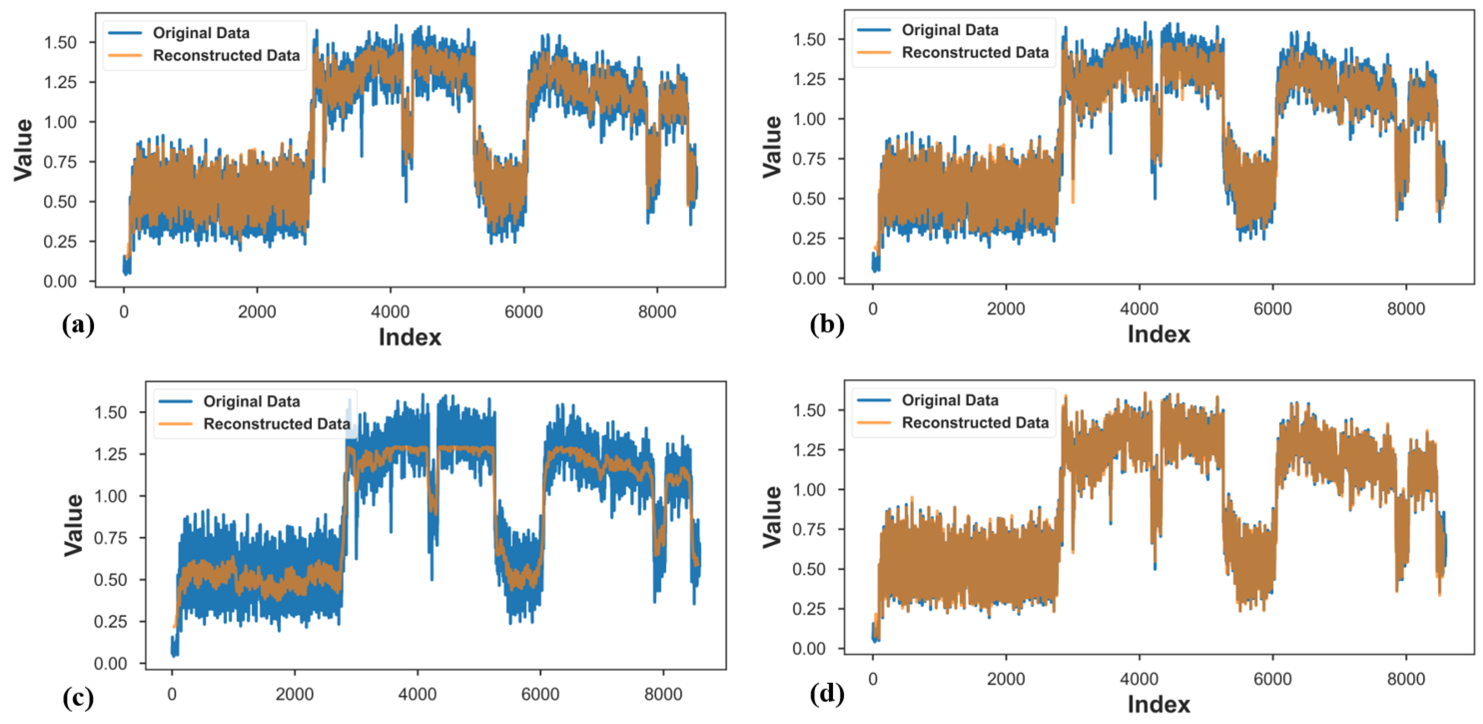
Interestingly, by comparing the original and reconstructed data as shown in Figure 10a–d, we can assess the accuracy of the AD framework. Anomalies detected in the DLAE model correspond to discrepancies between the original data and reconstructed data across the LSTM, GRU, and CNN models, with the RNN showing little or low glimpses of reconstructing the original data. Additionally, as observed in the figure, the DLAE models comprising the LSTM, GRU, and CNN validated the severity of detected anomalies. Moreover, the RNN showed larger discrepancies between the original and the reconstructed data, which showed the model performing poorly.
The following bar plot in Figure 11a depicts the performance of four models (LSTM, GRU, RNN, and CNN) based on three error metrics: MSE, MAE, and RMSE. Upon examining the bar plot, it is evident that for all three error metrics:
- MSE: The CNN model has the lowest MSE, followed closely by the GRU model. The LSTM and RNN models exhibit slightly higher MSE values than GRU and LSTM.
- MAE: Similar to MSE, the CNN model achieves the lowest MAE, indicating better performance in terms of average absolute error. Again, the GRU model closely follows the CNN model regarding performance. The LSTM and RNN models have higher MAE values than GRU and CNN.
- RMSE: The CNN model also demonstrates the lowest RMSE, signifying superior performance regarding the root mean squared error. Once more, the GRU model closely trails the CNN model in performance. The RNN and LSTM models exhibit higher RMSE values than GRU and CNN.
Based on the bar plot, it is evident that the CNN model consistently outperforms the other models across all three error metrics, indicating its superiority in terms of predictive accuracy. The GRU model closely follows the CNN model in terms of performance. On the other hand, the RNN and LSTM models exhibit higher error values, suggesting relatively poorer performance than GRU and CNN. Therefore, the bar plot highlights the CNN model as the best-performing model among the four considered in this analysis regarding predictive accuracy and error minimization. On the other hand, the RNN and LSTM models exhibit relatively inferior performance.
Heatmap analysis: As shown in Figure 11b, the heatmap provides a comprehensive overview of the model performances across different error metrics. The CNN model consistently outperforms the other models across all metrics, displaying the lowest error values for MSE, MAE, and RMSE. The GRU model closely follows the CNN model in performance, demonstrating slightly higher error values, but still outperforming the LSTM and RNN models. The LSTM and RNN models exhibit relatively higher error values across all metrics, indicating inferior performance compared to CNN and GRU.
Box plot analysis: Besides the heatmap analysis, the box plot, as shown in Figure 11c, provides insights into the variability of error values for each model across the three metrics. Consistent with the heatmap findings, the CNN model showcases the smallest spread of error values, indicating more consistent performance. The GRU model follows closely in performance, displaying slightly higher variability but still outperforming the LSTM and RNN models. The LSTM and RNN models exhibit higher variability in error values, reflecting less consistent performance than GRU and CNN.
Overall implications: Both visualizations confirm the superiority of the CNN model in predictive accuracy, as it consistently achieves the lowest error values and demonstrates minor variability across all error metrics. The GRU model also performs competitively, while the LSTM and RNN models exhibit less consistent performance and higher error variability. Integrating insights from the heatmap and box plot provides a comprehensive understanding of the model’s performance and valuable guidance for selecting the most effective deep-learning model. A detailed comparison of the overall MAE, MSE, and RMSE results is provided in Table 2 for a comprehensive assessment of the model’s predictive capabilities.
5. Limitations and Open Issues
Combining autoencoders with deep learning models like LSTM, GRU, RNN, and CNN is a reliable feature learning and AD approach across various applications, including predictive maintenance. However, this method faces several challenges and open issues. One significant challenge is the poor quality and sensitivity of the collected vibration signals. Low-sensitivity signals can result in noisy data, making it difficult for the models to learn meaningful representations and accurately detect anomalies [62].Additionally, the complex and high-dimensional nature of vibration data poses a challenge for dimensionality reduction techniques used by autoencoders. Balancing information compression with preserving important features is crucial yet challenging. Moreover, deep learning models’ computational complexity and training time can be significant, especially when combined with autoencoders. It poses practical challenges, particularly in real-time or resource-constrained environments [63].
Furthermore, interpreting these models’ learned representations and decision-making processes can be challenging, hindering trust and acceptance, particularly in critical domains like industrial systems [64]. Lastly, ensuring the generalization and adaptability of the models to unseen data or changing environments remains an ongoing challenge, requiring further study and innovation [65]. To address these challenges and open issues, advancements in data preprocessing, model architecture design, regularization techniques, and interpretability methods are necessary, alongside domain-specific knowledge and expertise.
6. Conclusions and Future Works
This study proposes a novel anomaly detection (AD) based on deep-learning autoencoders (DLAE). The proposed method uses vibration data from a speed reducer (SR) within adhesive coating equipment (ACE) under prolonged automobile bushing production. These are the main steps carried out in the proposed method: (1) A novel method is presented to assess the AD of SR using vibration data. We ensured the position of the NI 9234 sensor close to the bearing casing of the SR to help capture the normal and faulty patterns from the SR during its working conditions. (2) DLAE is utilized to perform the AD of the SR. The experiment showcases that the method effectively detects anomalies from the vibration signals. Our DLAE model captures long-term dependencies in time series data with a comparative assessment between the DLAE models. The autoencoder generates encoded features while preserving these dependencies. The MAE from training the model serves as the threshold for AD. Observations with reconstruction loss exceeding the threshold are flagged as anomalies during testing. The anomalies detected through the DLAE models give insight into replacing the chain within the ACE.
For future works, we would delve into two methodologies: (1) Optimizing sensor placement and integrating multi-sensor data are essential to improving the effectiveness of AD systems. By placing sensors in the correct positions, comprehensive vibration data can be captured, reflecting the actual health status of the equipment. (2) Integrating data from multiple sensors strategically positioned across different equipment components can provide a more holistic view of the equipment’s health. Leveraging advanced techniques in sensor fusion and data integration can also extract valuable insights from the collective information gathered, enhancing the AD system’s overall predictive capabilities.
Author Contributions
Conceptualization S.L. and A.B.K. methodology S.L. and A.B.K.; software S.L., A.B.K. and J.-W.H.; validation S.L. and A.B.K.; formal analysis S.L. and A.B.K.; investigation S.L. and A.B.K.; data curation S.L. and A.B.K.; writing—original draft preparation A.B.K.; writing—review and editing A.B.K.; and visualization S.L. and A.B.K.; resources and supervision J.-W.H.; project administration J.-W.H.; and funding acquisition J.-W.H. All authors have read and agreed to the published version of the manuscript.
Funding
This work was supported by the Innovative Human Resource Development for Local Intellectualization program through the Institute of Information & Communications Technology Planning & Evaluation(IITP) grant funded by the Korean government(MSIT) (IITP-2024-2020-0-01612).
Institutional Review Board Statement
Not applicable.
Informed Consent Statement
Not applicable.
Data Availability Statement
The data presented in this study are available on request from the corresponding author. The data are not publicly available due to laboratory regulations.
Conflicts of Interest
The authors declare no conflicts of interest.
Abbreviations
The following abbreviations are used in this manuscript:
| AD | Anomaly detection |
| ACE | Adhesive coating equipment |
| CNN | Convolutional Neural Networks |
| CSV | Comma separated values |
| DLAE | Deep learning autoencoder |
| GRU | Gated recurrent units |
| LSTM | Long Short-Term Memory |
| MAE | Mean absolute error |
| METL | Mechanisms engineering test loop |
| MSE | Mean square error |
| SGD | Stochastic gradient descent |
| RET | Reconstruction Error Threshold |
| RMSE | Root mean square error |
| RNN | Recurrent Neural Network |
| SR | Speed reducer |
| VFA | Variational fuzzy autoencoders |
References
- Pech, M.; Vrchota, J.; Bednář, J. Predictive Maintenance and Intelligent Sensors in Smart Factory: Review. Sensors 2021, 21, 1470. [Google Scholar] [CrossRef] [PubMed]
- Çınar, Z.M.; Abdussalam Nuhu, A.; Zeeshan, Q.; Korhan, O.; Asmael, M.; Safaei, B. Machine Learning in Predictive Maintenance towards Sustainable Smart Manufacturing in Industry 4.0. Sustainability 2020, 12, 8211. [Google Scholar] [CrossRef]
- Molęda, M.; Małysiak-Mrozek, B.; Ding, W.; Sunderam, V.; Mrozek, D. From Corrective to Predictive Maintenance—A Review of Maintenance Approaches for the Power Industry. Sensors 2023, 23, 5970. [Google Scholar] [CrossRef] [PubMed]
- Achouch, M.; Dimitrova, M.; Ziane, K.; Sattarpanah Karganroudi, S.; Dhouib, R.; Ibrahim, H.; Adda, M. On Predictive Maintenance in Industry 4.0: Overview, Models, and Challenges. Appl. Sci. 2022, 12, 8081. [Google Scholar] [CrossRef]
- Gorla, C.; Davoli, P.; Rosa, F.; Longoni, C.; Chiozzi, F.; Samarani, A. Theoretical and Experimental Analysis of a Cycloidal Speed Reducer. ASME J. Mech. Des. 2008, 130, 112604. [Google Scholar] [CrossRef]
- Hermes, G.; Simone, C.; Giovanni, L. A Practical Approach to the Selection of the Motor-Reducer Unit in Electric Drive Systems. Mech. Based Des. Struct. Mach. 2011, 39, 303–319. [Google Scholar] [CrossRef]
- Giberti, H.; Cinquemani, S.; Legnani, G. Effects of transmission mechanical characteristics on the choice of a motor-reducer. Mechatronics 2010, 20, 604–610. [Google Scholar] [CrossRef]
- Teng, W.; Ding, X.; Tang, S.; Xu, J.; Shi, B.; Liu, Y. Vibration Analysis for Fault Detection of Wind Turbine Drivetrains—A Comprehensive Investigation. Sensors 2021, 21, 1686. [Google Scholar] [CrossRef] [PubMed]
- Kafeel, A.; Aziz, S.; Awais, M.; Khan, M.A.; Afaq, K.; Idris, S.A.; Alshazly, H.; Mostafa, S.M. An Expert System for Rotating Machine Fault Detection Using Vibration Signal Analysis. Sensors 2021, 21, 7587. [Google Scholar] [CrossRef] [PubMed]
- Tiboni, M.; Remino, C.; Bussola, R.; Amici, C. A Review on Vibration-Based Condition Monitoring of Rotating Machinery. Appl. Sci. 2022, 12, 972. [Google Scholar] [CrossRef]
- Cui, L.; Zhao, X.; Liu, D.; Wang, H. A spectral coherence cyclic periodic index optimization gram for bearing fault diagnosis. Measurement 2024, 224, 113898. [Google Scholar] [CrossRef]
- Du, W.; Yang, L.; Wang, H.; Gong, X.; Zhang, L.; Li, C.; Ji, L. LN-MRSCAE: A novel deep-learning-based denoising method for mechanical vibration signals. J. Vib. Control 2024, 30, 459–471. [Google Scholar] [CrossRef]
- Guishuai, F.; Qiang, L.; Tengfei, W.; David, P.C.; Kaiwen, L. Frequency Spectra Analysis of Vertical Stress in Ballasted Track Foundations: Influence of Train Configuration and Subgrade Depth. Transp. Geotech. 2024, 44, 101167. [Google Scholar] [CrossRef]
- Akpudo, U.E.; Jang-Wook, H. A Multi-Domain Diagnostics Approach for Solenoid Pumps Based on Discriminative Features. IEEE Access 2020, 8, 175020–175034. [Google Scholar] [CrossRef]
- Li, H.; Wang, D. Multilevel feature fusion of multi-domain vibration signals for bearing fault diagnosis. SIViP 2024, 18, 99–108. [Google Scholar] [CrossRef]
- Zeng, Y.; Zhang, J.; Zhong, Y.; Deng, L.; Wang, M. STNet: A Time-Frequency Analysis-Based Intrusion Detection Network for Distributed Optical Fiber Acoustic Sensing Systems. Sensors 2024, 24, 1570. [Google Scholar] [CrossRef]
- Li, E.; Jian, J.; Yang, F.; Ma, Z.; Hao, Y.; Chang, H. Characterization of Sensitivity of Time Domain MEMS Accelerometer. Micromachines 2024, 15, 227. [Google Scholar] [CrossRef]
- Pang, B.; Liu, Q.; Sun, Z.; Xu, Z.; Hao, Z. Time-frequency supervised contrastive learning via pseudo-labeling: An unsupervised domain adaptation network for rolling bearing fault diagnosis under time-varying speeds. Adv. Eng. Inform. 2024, 59, 102304. [Google Scholar] [CrossRef]
- Mafla-Yépez, C.; Castejon, C.; Rubio, H.; Morales, C. A Vibration Analysis for the Evaluation of Fuel Rail Pressure and Mass Air Flow Sensors on a Diesel Engine: Strategies for Predictive Maintenance. Sensors 2024, 24, 1551. [Google Scholar] [CrossRef]
- Meng, F.; Shi, Z.; Song, Y. A Novel Fault Diagnosis Strategy for Diaphragm Pumps Based on Signal Demodulation and PCA-ResNet. Sensors 2024, 24, 1578. [Google Scholar] [CrossRef]
- Shayan, G.; Hosseinzadeh, S.A.A. A novel unsupervised deep-learning approach for vibration-based damage diagnosis using a multi-head self-attention LSTM autoencoder. Measurement 2024, 229, 114410. [Google Scholar] [CrossRef]
- Fei, J.; Qin, L.; Zhaoqian, W.; Yicong, K.; Shaohui, Z.; Jinglun, L. A zero-cost unsupervised transfer method based on non-vibration signals fusion for ball screw fault diagnosis. Knowl.-Based Syst. 2024, 288, 111475. [Google Scholar] [CrossRef]
- Mao, W.; Wang, Y.; Feng, K.; Kou, L.; Zhang, Y. SWDAE: A New Degradation State Evaluation Method for Metro Wheels With Interpretable Health Indicator Construction Based on Unsupervised deep-learning. IEEE Trans. Instrum. Meas. 2024, 73, 3507313. [Google Scholar] [CrossRef]
- Zhang, T.; Zhou, L.; Li, J.; Niu, H. Health Management of Bearings Using Adaptive Parametric VMD and Flying Squirrel Search Algorithms to Optimize SVM. Processes 2024, 12, 433. [Google Scholar] [CrossRef]
- Seo, M.-K.; Yun, W.-Y. Gearbox Condition Monitoring and Diagnosis of Unlabeled Vibration Signals Using a Supervised Learning Classifier. Machines 2024, 12, 127. [Google Scholar] [CrossRef]
- Łuczak, D. Machine Fault Diagnosis through Vibration Analysis: Continuous Wavelet Transform with Complex Morlet Wavelet and Time–Frequency RGB Image Recognition via Convolutional Neural Network. Electronics 2024, 13, 452. [Google Scholar] [CrossRef]
- Zhang, Q.; Song, C.; Yuan, Y. Fault Diagnosis of Vehicle Gearboxes Based on Adaptive Wavelet Threshold and LT-PCA-NGO-SVM. Appl. Sci. 2024, 14, 1212. [Google Scholar] [CrossRef]
- Zhang, X.; He, W.; Cui, Q.; Bai, T.; Li, B.; Li, J.; Li, X. WavLoadNet: Dynamic Load Identification for Aeronautical Structures Based on Convolution Neural Network and Wavelet Transform. Appl. Sci. 2024, 14, 1928. [Google Scholar] [CrossRef]
- Akpudo, U.E.; Hur, J.-W. A Wavelet-Based Diagnostic Framework for CRD Engine Injection Systems under Emulsified Fuel Conditions. Electronics 2021, 10, 2922. [Google Scholar] [CrossRef]
- Okwuosa, C.N.; Hur, J.-W. An Intelligent Hybrid Feature Selection Approach for SCIM Inter-Turn Fault Classification at Minor Load Conditions Using Supervised Learning. IEEE Access 2023, 11, 89907–89920. [Google Scholar] [CrossRef]
- Qin, Y.-F.; Fu, X.; Li, X.-K.; Li, H.-J. ADAMS Simulation and HHT Feature Extraction Method for Bearing Faults of Coal Shearer. Processes 2024, 12, 164. [Google Scholar] [CrossRef]
- Zhenhua, N.; Fuquan, L.; Jun, L.; Hong, H.; Yizhou, L.; Hongwei, M. Baseline-free structural damage detection using PCA- Hilbert transform with limited sensors. J. Sound Vib. 2024, 568, 117966. [Google Scholar] [CrossRef]
- Song, Y.; Hyun, S.; Cheong, Y.-G. Analysis of Autoencoders for Network Intrusion Detection. Sensors 2021, 21, 4294. [Google Scholar] [CrossRef] [PubMed]
- Chen, S.; Guo, W. Auto-Encoders in deep-learning—A Review with New Perspectives. Mathematics 2023, 11, 1777. [Google Scholar] [CrossRef]
- Karim, A.M.; Kaya, H.; Güzel, M.S.; Tolun, M.R.; Çelebi, F.V.; Mishra, A. A Novel Framework Using Deep Auto-Encoders Based Linear Model for Data Classification. Sensors 2020, 20, 6378. [Google Scholar] [CrossRef] [PubMed]
- Rosafalco, L.; Manzoni, A.; Mariani, S.; Corigliano, A. An Autoencoder-Based deep-learning Approach for Load Identification in Structural Dynamics. Sensors 2021, 21, 4207. [Google Scholar] [CrossRef] [PubMed]
- Pisa, I.; Morell, A.; Vicario, J.L.; Vilanova, R. Denoising Autoencoders and LSTM-Based Artificial Neural Networks Data Processing for Its Application to Internal Model Control in Industrial Environments—The Wastewater Treatment Plant Control Case. Sensors 2020, 20, 3743. [Google Scholar] [CrossRef] [PubMed]
- Miranda-González, A.A.; Rosales-Silva, A.J.; Mújica-Vargas, D.; Escamilla-Ambrosio, P.J.; Gallegos-Funes, F.J.; Vianney-Kinani, J.M.; Velázquez-Lozada, E.; Pérez-Hernández, L.M.; Lozano-Vázquez, L.V. Denoising Vanilla Autoencoder for RGB and GS Images with Gaussian Noise. Entropy 2023, 25, 1467. [Google Scholar] [CrossRef] [PubMed]
- Junges, R.; Lomazzi, L.; Miele, L.; Giglio, M.; Cadini, F. Mitigating the Impact of Temperature Variations on Ultrasonic Guided Wave-Based Structural Health Monitoring through Variational Autoencoders. Sensors 2024, 24, 1494. [Google Scholar] [CrossRef]
- La Grassa, R.; Re, C.; Cremonese, G.; Gallo, I. Hyperspectral Data Compression Using Fully Convolutional Autoencoder. Remote Sens. 2022, 14, 2472. [Google Scholar] [CrossRef]
- Cong, X.; Shicheng, Z.; Yuanlin, H.; Xiaolong, G.; Xingfang, M.; Tong, Z.; Jianbing, J. Robust optimization of geo-energy production using data-driven deep recurrent auto-encoder and fully-connected neural network proxy. Expert Syst. Appl. 2024, 242, 122797. [Google Scholar] [CrossRef]
- Saminathan, K.; Mulka, S.T.R.; Damodharan, S.; Maheswar, R.; Lorincz, J. An Artificial Neural Network Autoencoder for Insider Cyber Security Threat Detection. Future Internet 2023, 15, 373. [Google Scholar] [CrossRef]
- Alsaade, F.W.; Al-Adhaileh, M.H. Cyber Attack Detection for Self-Driving Vehicle Networks Using Deep Autoencoder Algorithms. Sensors 2023, 23, 4086. [Google Scholar] [CrossRef] [PubMed]
- Singh, A.; Ogunfunmi, T. An Overview of Variational Autoencoders for Source Separation, Finance, and Bio-Signal Applications. Entropy 2022, 24, 55. [Google Scholar] [CrossRef] [PubMed]
- Albahli, S.; Nazir, T.; Mehmood, A.; Irtaza, A.; Alkhalifah, A.; Albattah, W. AEI-DNET: A Novel DenseNet Model with an Autoencoder for the Stock Market Predictions Using Stock Technical Indicators. Electronics 2022, 11, 611. [Google Scholar] [CrossRef]
- Bampoula, X.; Siaterlis, G.; Nikolakis, N.; Alexopoulos, K. A deep-learning Model for Predictive Maintenance in Cyber-Physical Production Systems Using LSTM Autoencoders. Sensors 2021, 21, 972. [Google Scholar] [CrossRef] [PubMed]
- Ribeiro, D.; Matos, L.M.; Moreira, G.; Pilastri, A.; Cortez, P. Isolation Forests and Deep Autoencoders for Industrial Screw Tightening AD. Computers 2022, 11, 54. [Google Scholar] [CrossRef]
- Kaupp, L.; Humm, B.; Nazemi, K.; Simons, S. Autoencoder-Ensemble-Based Unsupervised Selection of Production-Relevant Variables for Context-Aware Fault Diagnosis. Sensors 2022, 22, 8259. [Google Scholar] [CrossRef]
- Mehta, D.; Klarmann, N. Autoencoder-Based Visual Anomaly Localization for Manufacturing Quality Control. Mach. Learn. Knowl. Extr. 2024, 6, 1–17. [Google Scholar] [CrossRef]
- García-Ordás, M.T.; Benítez-Andrades, J.A.; García-Rodríguez, I.; Benavides, C.; Alaiz-Moretón, H. Detecting Respiratory Pathologies Using Convolutional Neural Networks and Variational Autoencoders for Unbalancing Data. Sensors 2020, 20, 1214. [Google Scholar] [CrossRef]
- Xu, W.; He, J.; Li, W.; He, Y.; Wan, H.; Qin, W.; Chen, Z. Long-Short-Term-Memory-Based Deep Stacked Sequence-to-Sequence Autoencoder for Health Prediction of Industrial Workers in Closed Environments Based on Wearable Devices. Sensors 2023, 23, 7874. [Google Scholar] [CrossRef]
- Kang, J.; Kim, C.-S.; Kang, J.W.; Gwak, J. AD of the Brake Operating Unit on Metro Vehicles Using a One-Class LSTM Autoencoder. Appl. Sci. 2021, 11, 9290. [Google Scholar] [CrossRef]
- Bono, F.M.; Radicioni, L.; Cinquemani, S.; Bombaci, G. A Comparison of deep-learning Algorithms for AD in Discrete Mechanical Systems. Appl. Sci. 2023, 13, 5683. [Google Scholar] [CrossRef]
- Wei, J. A Machine Vision AD System to Industry 4.0 Based on Variational Fuzzy Autoencoder. Comput. Intell. Neurosci. 2022, 2022, 1945507. [Google Scholar] [CrossRef] [PubMed]
- Akins, A.; Kultgen, D.; Heifetz, A. AD in Liquid Sodium Cold Trap Operation with Multisensory Data Fusion Using Long Short-Term Memory Autoencoder. Energies 2023, 16, 4965. [Google Scholar] [CrossRef]
- Rollo, F.; Bachechi, C.; Po, L. AD and Repairing for Improving Air Quality Monitoring. Sensors 2023, 23, 640. [Google Scholar] [CrossRef] [PubMed]
- Marco, P.; Giuseppe, D.-P.; Massimo, E. Real-time AD on time series of industrial furnaces: A comparison of autoencoder architectures. Eng. Appl. Artif. Intell. 2023, 124, 106597. [Google Scholar] [CrossRef]
- Patra, K.; Sethi, R.N.; Behera, D.K. AD in rotating machinery using autoencoders based on bidirectional LSTM and GRU neural networks. Turk. J. Electr. Eng. Comput. Sci. 2022, 30, 30. [Google Scholar] [CrossRef]
- Mikel, C.; Isaac, T.; Angel, C.; Enrique, O. Multi-head CNN–RNN for multi-time series AD: An industrial case study. Neurocomputing 2019, 363, 246–260. [Google Scholar] [CrossRef]
- Khan, S.W.; Hafeez, Q.; Khalid, M.I.; Alroobaea, R.; Hussain, S.; Iqbal, J.; Almotiri, J.; Ullah, S.S. AD in Traffic Surveillance Videos Using deep-learning. Sensors 2022, 22, 6563. [Google Scholar] [CrossRef]
- Do, J.S.; Kareem, A.B.; Hur, J.-W. LSTM-Autoencoder for Vibration AD in Vertical Carousel Storage and Retrieval System (VCSRS). Sensors 2023, 23, 1009. [Google Scholar] [CrossRef]
- Esmaeili, F.; Cassie, E.; Nguyen, H.P.T.; Plank, N.O.V.; Unsworth, C.P.; Wang, A. AD for Sensor Signals Utilizing Deep Learning Autoencoder-Based Neural Networks. Bioengineering 2023, 10, 405. [Google Scholar] [CrossRef] [PubMed]
- Ajani, T.S.; Imoize, A.L.; Atayero, A.A. An Overview of Machine Learning within Embedded and Mobile Devices–Optimizations and Applications. Sensors 2021, 21, 4412. [Google Scholar] [CrossRef]
- Linardatos, P.; Papastefanopoulos, V.; Kotsiantis, S. Explainable AI: A Review of Machine Learning Interpretability Methods. Entropy 2021, 23, 18. [Google Scholar] [CrossRef] [PubMed]
- Taye, M.M. Understanding of Machine Learning with Deep Learning: Architectures, Workflow, Applications and Future Directions. Computers 2023, 12, 91. [Google Scholar] [CrossRef]
Figure 1.
An overview of the adhesive coating equipment. (a) The bushing undergoes a controlled heating process within a preheated oven to maintain a uniform surface temperature. (b) Subsequently, it is conveyed to a designated spray booth where the atomized adhesive (Chemlok 6108) is applied onto the inner surface of the tube via a specialized nozzle. (c) Following that application, the bushing proceeds through a base coat drying oven to undergo a drying cycle. (d) After the base coat stage, the bushing advances to another spray booth, where a topcoat of adhesive (Chemlok 205 + MIBK) is administered using a similar method employed in the previous stage. (e) Finally, the topcoat undergoes drying within a dedicated oven, mirroring the drying process observed in the preceding stage.

Figure 2.
A flow diagram of a GRU neural network model showcasing its internal gating mechanisms for memory and information flow control in sequential data processing.
Figure 2.
A flow diagram of a GRU neural network model showcasing its internal gating mechanisms for memory and information flow control in sequential data processing.

Figure 3.
A flow diagram illustrating the Long Short-Term Memory (LSTM) neural network model.

Figure 4.
Proposed model architecture illustrating the DLAE components for AD.

Figure 5.
Experiment view capturing the vibration sensor, electric motor, and speed reducer.

Figure 6.
Visualization of the vibration raw data from the speed reducer.

Figure 7.
Plot showing the original data alongside detected anomalies. (a) Raw data, (b) normalized data.
Figure 7.
Plot showing the original data alongside detected anomalies. (a) Raw data, (b) normalized data.

Figure 8.
Comparison of training and validation loss (a) LSTM, (b) GRU, (c) RNN, (d) CNN.

Figure 9.
Anomalies detected using an autoencoder-based approach for LSTM, GRU, RNN, and CNN models. The plot showcases highlighted regions indicating abnormal patterns in the data, aiding in predictive maintenance and system health monitoring. (a) LSTM, (b) GRU, (c) RNN, (d) CNN.
Figure 9.
Anomalies detected using an autoencoder-based approach for LSTM, GRU, RNN, and CNN models. The plot showcases highlighted regions indicating abnormal patterns in the data, aiding in predictive maintenance and system health monitoring. (a) LSTM, (b) GRU, (c) RNN, (d) CNN.

Figure 10.
Reconstruction plot showcasing the performance of LSTM, GRU, RNN, and CNN autoencoders in capturing anomalies within vibration data from industrial machinery. Each curve represents the reconstructed data overlaid with the original signal, demonstrating the efficacy of each model in capturing anomalies and preserving signal characteristics. (a) LSTM, (b) GRU, (c) RNN, (d) CNN.

Figure 11.
Side-by-side comparison of performance metrics (MSE, MAE, RMSE) across various deep-learning models, illustrated with a (a) bar plot, (b) heatmap, (c) box plot.
Figure 11.
Side-by-side comparison of performance metrics (MSE, MAE, RMSE) across various deep-learning models, illustrated with a (a) bar plot, (b) heatmap, (c) box plot.


Table 1.
DLAE model architecture parameters.
| Model | Parameters | Values |
|---|---|---|
| LSTM, GRU | Units (Encoder) | 512, 256, 128, 64, 32 |
| Units (Decoder) | 32, 64, 128, 256, 512 | |
| Activation function | tanh | |
| Dropout rate | 0.1 | |
| Batch Size | 512, 128 | |
| Epoch | 50 | |
| Validation Split | 0.1 | |
| CNN | Units (Encoder) | 128, 64, 32 |
| Pooling (Encoder) | 2 × 2 Max Pooling | |
| Units (Decoder) | 32, 64, 128 | |
| Pooling (Decoder) | 2 × 2 UpSampling | |
| Activation function | ReLU | |
| Dropout rate | 0.1 | |
| Batch Size | 128 | |
| Epoch | 50 | |
| Validation Split | 0.1 | |
| Kernel Size | 3 | |
| RNN | Units (Encoder) | 128, 64, 32 |
| Units (Decoder) | 32, 64, 128 | |
| Activation function | tanh | |
| Dropout rate | 0.1 | |
| Batch Size | 128 | |
| Epoch | 50 | |
| Validation Split | 0.1 |
Table 2.
Global performance comparison of DLAE models.
| Model | MSE (%) | MAE (%) | RMSE (%) | RET * |
|---|---|---|---|---|
| LSTM | 0.2841 | 0.4130 | 0.5539 | 0.0562 |
| GRU | 0.2676 | 0.4186 | 0.5076 | 0.0539 |
| RNN | 0.2983 | 0.4661 | 0.5982 | 0.1806 |
| CNN | 0.2643 | 0.4115 | 0.5037 | 0.0201 |
* Reconstruction Error Threshold
Disclaimer/Publisher’s Note: The statements, opinions and data contained in all publications are solely those of the individual author(s) and contributor(s) and not of MDPI and/or the editor(s). MDPI and/or the editor(s) disclaim responsibility for any injury to people or property resulting from any ideas, methods, instructions or products referred to in the content. |
© 2024 by the authors. Licensee MDPI, Basel, Switzerland. This article is an open access article distributed under the terms and conditions of the Creative Commons Attribution (CC BY) license (https://creativecommons.org/licenses/by/4.0/).
Share and Cite
MDPI and ACS Style
Lee, S.; Kareem, A.B.; Hur, J.-W. A Comparative Study of Deep-Learning Autoencoders (DLAEs) for Vibration Anomaly Detection in Manufacturing Equipment. Electronics 2024, 13, 1700. https://doi.org/10.3390/electronics13091700
AMA Style
Lee S, Kareem AB, Hur J-W. A Comparative Study of Deep-Learning Autoencoders (DLAEs) for Vibration Anomaly Detection in Manufacturing Equipment. Electronics. 2024; 13(9):1700. https://doi.org/10.3390/electronics13091700
Chicago/Turabian StyleLee, Seonwoo, Akeem Bayo Kareem, and Jang-Wook Hur. 2024. "A Comparative Study of Deep-Learning Autoencoders (DLAEs) for Vibration Anomaly Detection in Manufacturing Equipment" Electronics 13, no. 9: 1700. https://doi.org/10.3390/electronics13091700
Note that from the first issue of 2016, this journal uses article numbers instead of page numbers. See further details here.