Article

Innovative Artificial Intelligence Approach for Hearing-Loss Symptoms Identification Model Using Machine Learning Techniques

by
Mohd Khanapi Abd Ghani
1,
Nasir G. Noma
2,
Mazin Abed Mohammed
3,*,
Karrar Hameed Abdulkareem
4,
Begonya Garcia-Zapirain
5,*,
Mashael S. Maashi
6 and
Salama A. Mostafa
7
1
Biomedical Computing and Engineering Technologies (BIOCORE) Applied Research Group, Faculty of Information and Communication Technology, Universiti Teknikal Malaysia Melaka, Melaka 76100, Malaysia
2
Research & Development Department, Nigerian Communications Commission, Abuja FCT 257776, Nigeria
3
Information Systems Department, College of Computer Science and Information Technology, University of Anbar, Ramadi, Anbar 31001, Iraq
4
College of Agriculture, Al-Muthanna University, Samawah 66001, Iraq
5
eVIDA Lab, University of Deusto, Avda/Universidades 24, 48007 Bilbao, Spain
6
Software Engineering Department, College of Computer and Information Sciences, King Saud University, Riyadh 11451, Saudi Arabia
7
Faculty of Computer Science and Information Technology, Universiti Tun Hussein Onn Malaysia, Batu Pahat 86400, Malaysia
*
Authors to whom correspondence should be addressed.
Sustainability 2021, 13(10), 5406; https://doi.org/10.3390/su13105406
Submission received: 19 March 2021 / Revised: 7 May 2021 / Accepted: 9 May 2021 / Published: 12 May 2021

Abstract

:
Physicians depend on their insight and experience and on a fundamentally indicative or symptomatic approach to decide on the possible ailment of a patient. However, numerous phases of problem identification and longer strategies can prompt a longer time for consulting and can subsequently cause other patients that require attention to wait for longer. This can bring about pressure and tension concerning those patients. In this study, we focus on developing a decision-support system for diagnosing the symptoms as a result of hearing loss. The model is implemented by utilizing machine learning techniques. The Frequent Pattern Growth (FP-Growth) algorithm is used as a feature transformation method and the multivariate Bernoulli naïve Bayes classification model as the classifier. To find the correlation that exists between the hearing thresholds and symptoms of hearing loss, the FP-Growth and association rule algorithms were first used to experiment with small sample and large sample datasets. The result of these two experiments showed the existence of this relationship, and that the performance of the hybrid of the FP-Growth and naïve Bayes algorithms in identifying hearing-loss symptoms was found to be efficient, with a very small error rate. The average accuracy rate and average error rate for the multivariate Bernoulli model with FP-Growth feature transformation, using five training sets, are 98.25% and 1.73%, respectively.

1. Introduction

More than 5 percent (466 million) of the world’s population is affected by hearing loss (432 million adults, 34 million children). It is predicted that over 900 million people, or one out of ten, will experience hearing loss by 2050 [1]. Restricted hearing loss is more than 40 decibels (dB) in the better ear of an adult and more than 30 dB in that of a child. Most people living in low- and middle-income countries suffer from hearing loss [1]. Around a third of people over the age of 65 suffer from disabling hearing loss. In South Asia, the Asia Pacific and sub-Saharan Africa, the frequency of this age group is greatly increased. Statistics show that in the Asia Pacific, an area of which Malaysia is part, the occurrence of affected hearing loss is very high [2]. About 31,000 hearing loss cases were reported in Malaysia alone during 1980. In 2005, national survey disorder statistics indicate that the population prevalence was 17.4%, and during this time about 3,962,879 cases were reported. The Ministry of Health of Malaysia reported hearing loss as one of the top 10 illnesses [3].
Hearing loss is among the most prominent diseases harming children as well as younger and older adults, and can contribute to impairment if they are not properly diagnosed early. An otorhinolaryngologist categorizes the symptoms of a patient according to his/her expertise and after the specific evaluation of the symptoms of hearing loss. Such procedures include five steps followed by an order, which include a collection of patient case history, otoscopy, audiometric hearing tests, tympanometry and acoustic reflex. Given the number of patients who usually visit ENT departments of various hospitals to get their hearing problem treated and the amount of time it takes for each procedure to be performed during a consultation with the otorhinolaryngologist, these phases may delay treatment process and makes patients leaving the hospital because they already waited for a long time [4]. A long waiting time can cause anxiety and stress in the patients in the queue [5]. The patients’ understanding of the health system, therefore, tampers with possible solutions, and thus it is important to reduce the average waiting time of patients so that the overall cost of consulting hearing-loss patients is reduced [6,7,8]. Procedures or measures to evaluate hearing loss in patients are available. The first step in the investigation is pure tone audiometry [9]. Hearing tests are carried out in a room that is very quiet and noise-free. Sounds are conveyed by audiologists on earphones at various frequencies (250–8000 Hz) and sound intensities (−10–140 dB), who advises the patient to hit the button for the least possible-to-hear sound. The test results are recorded on a soundtrack.
Figure 1 displays the hearing loss investigation approach. On a patient’s first appointment, physicians refer him to an ENT specialist. Once hearing issues begin, the physician will ask for the case history of one of the most common and basic audiological tests for hearing loss, making differential diagnoses possible with the patient’s case history [10]. The following test will be done using an otoscope; the physician will then visually examine the external auditory channel [11]. The ENT professional then refers the patient to an audiologist who examines the patient’s hearing loss by using an audiometer, integrating clarity of tone at various frequencies. In conjunction with an examination, tympanometry helps physicians to assess how well the conducting pathway passes sounds to the inner ear. Acoustic reflexes test stapedial muscle contraction in the middle ear to respond to severe sound [12]. During all of the following examination stages, the physician can diagnose whether it is conductive hearing loss, sensorineural or mixed hearing loss or normal hearing sensitivity to the illnesses or diseases that cause patients to lose their hearing ability. If conductive or mixed hearing loss occurs, the patient must go for a follow-up audiological evaluation after therapy by an ENT specialist. The ENT practitioner should create an auditory aid trail for the patient that is influenced by the way it is used and managed concerning sensorineural hearing loss. The ENT physician also organizes schedules with the patient after a few months or weeks for further evaluation [13]. The basic diagnosis and assessment protocol of hearing-loss symptoms for a patient with a hearing problem is illustrated in Figure 2.
Figure 2 illustrates the basic diagnosis and assessment protocol of hearing-loss symptoms for a patient with a hearing problem. Without these fundamental procedures, every audiological evaluation process is incomplete to determine the symptoms and type of hearing loss experienced by the patient [14]. Such five medical symptoms of hearing loss listed above are essential and fundamental clinical audiological medical techniques. One should disregard the amount of time spent on the procedures given their significance in diagnosing the forms and symptoms of hearing loss. The study carried out by [15] demonstrates that it takes a great deal of time to collect case history alone but offers interesting information. To treat certain waiting patients, the diagnostic process must always be accelerated. If a variety of tests are needed before the diagnosis findings are obtained by the specialist, then this may directly impact certain patients to be treated. Another study by [16] implies that a physician can classify signs of hearing loss considerably based on the case history and otoscopy. This reveals that the diagnostic protocol can be minimized and yet the expert can understand the issue by following all processes. Because numerous studies have shown how symptoms of hearing loss are linked to certain variations in the audiogram, a specialist may determine the form and symptoms of the hearing loss without necessarily performing all the diagnostic procedures using air and bone transmission.
The main objective of the study is to identify signs of hearing loss efficacy from the threshold of pure-tone air and bone conduction so that hearing loss is easier to investigate. This method includes identifying and using associations between pure sound audiometry and the signs and other features in the patient’s health audiology datasets to classify symptoms of hearing loss. The symptoms can indeed be precisely predicted using a diagnosis model that uses hybrid machine learning approaches, which can predict a class of pure audiometric data for the input air or bone conduction. Vast quantities of untapped and potentially useful data produced by healthcare providers have potential information. In determining the symptoms of a disease, medical professionals depend on their experience and knowledge and a practical diagnostic mechanism. Many diagnostic stages and longer procedures will lead to longer appointments, which means that those waiting to be treated have a longer time to wait. This can contribute to anxiety and stress in these patients. However, the contribution of our study can be seen as follows:
  • This work provides an important opportunity to boost the diagnostic process of hearing-loss symptoms by proposing a model of symptom detection to accurately classify symptoms of hearing loss based on pure audiometry data from air and bone conduction. The symptoms can indeed be precisely predicted using a diagnosis model that uses hybrid machine learning approaches, which can predict a class of pure audiometric data for the input air or bone conduction.
  • The model is implemented using Frequent Pattern Growth (FP-Growth) and the naïve Bayes (NB) algorithm, where FP-Growth is an unsupervised method that used for the feature extraction purpose while NB models are supervised models that are hired for the classification target.
  • FP-Growth was first applied with small sample and large sample datasets to analyze the correlation among both the hearing thresholds and symptoms of hearing loss. The results of these experiments showed hybridization of the FP-Growth and NB models, shown to work effectively with a very low error rate to determine hearing-loss symptoms.
The organization of this paper is as follows: Section 2 presents the related work for hearing loss identification. Section 3 describes the Materials and Methods for the classification of the hearing-loss symptoms identification model. The experimental results obtained are discussed in Section 4. The study constraints and limitations are discussed in Section 5. The conclusion of this study is made in Section 6.

2. Related Work

Numerous studies have developed hearing loss strategies or techniques that can boost or ease the role of otolaryngology clinicians. To aid physicians with hearing loss diagnosis [17], cluster forms of audiograms in homogenous and inhomogeneous clusters are applied using the K-mean technique for diagnosing hearing loss. Their research used pure tone data from 1633 individuals. The audiogram format was categorized by the K-means clustering algorithm in different cluster numbers, namely, 4, 5, 6, 7, 8, 9, 10 and 11. ANOVA, to test the presumption of homogeneity between the audiogram styles, was used to evaluate the clusters and the results were tested using the mentioned tool. The researchers in this study show that the judgment of a clinician during the diagnosis is based on their personal experiences that are not free of errors. Besides, there is a need for a consistent audiogram classification that can aid doctors in the diagnosis. The researchers did not reveal any pathology, signs, or frequency in relation to the classification of these audiograms. This correlation allows clinicians to understand the connection between other audiogram types and the characteristics of certain patients.
Moein et al. [18] has built a decision-support system for the evaluation of symptoms of hearing loss. Throughout their study, 150 patients from an otolaryngology clinic had been gathered. The Multi-Layer Perceptron Neural Network (MLP) and Support Vector Machine (SVM) were used for classification of hearing loss signs in six classes, namely, serous otitis media, otitis media, conductive fixation, cochlear age, cochlear noise and normal. The ear condition frequency in the dataset and the given labels for the MLP and SVM are displayed in Table 1.
Table 1 displays each ear condition frequency in the dataset and the given labels for the MLP and SVM. According to the results of the study, in the data classification, the SVM is stronger than the MLP, where SVM help achieving a 92.5% accuracy compared to MLP, with an accuracy of 77.5%. Despite the high SVM accuracy that can enhance patient diagnosis, only patients with particular or few symptoms or a disorder numbering to six were included in the experiments for small datasets. A dataset that would contain more typical signs would be more fitting and would have been better tested to determine the efficacy of the SVM on hearing-loss symptoms. Additionally, the Otoneurological System was created by [19] to help identify vertigo hearing-loss symptoms. To assess the accuracy of the machine training techniques and the accuracy of classification, the combination of the knowledge learned from machine learning techniques with expert knowledge to obtain information from the patient data, which will help with the diagnosis, the researchers focused on testing the mechanism of nearest K and naive Bayes classification techniques. An otoneurological dataset consisting of 815 experimental cases were collected. The data collection reveals acoustic neurinoma, Meniere’s disease, benign positional vertigo, sudden deafness, traumatic vertigo and vestibular neuritis. The researchers have used an extra 1030 cases of a vertigo dataset collected from the Helsinki University Central Hospital in the process of evaluating the accuracy of these techniques. In the study, two vertigo datasets were used for the technique of knowledge exploration and a comparison was made with the otolaryngologist’s knowledge. To assess the influence of both the otolaryngology information and the results of the machine learning technology, the classification accuracy is often combined in different ways. The findings showed the highest accuracy of classification by combining otolaryngologist knowledge with professional knowledge. The system was intended only for diagnosis of vertigo symptoms and more focus was put on testing the dataset system that only comprises vertigo cases. The method used to estimate the predictive accuracy of the information gained from the learning method was another drawback of this experiment. Approximately 70% of cases were used for algorithms training and only 30% were used for testing [19]. Thompson et al. [20] used a medical records database to find information on the causes and treatments of tinnitus to enhance tinnitus detection, interpretation of outcomes and an overall understanding. This is also the study that established a diagnostic method for the diagnosis of a single hearing loss symptom.
The diagnostic model for the identification of vestibular schwannomas from audiometric data has been developed and validated by [21], a company that provides an online audiometric hearing test service, by using an online application to play a range of tones at varying levels to the users whom will be asked to select the particular tones they can hear. A report of the result will be sent to them to view in AudioGen, which is a method that contains machine learning techniques to determine the genetic cause of hearing loss in people segregating autosomal prevalent non-individual hearing loss using phenotypical information derived from audiometric data. The study results show the predictability of the causative gene within the three top predictions, with an algorithm accuracy at 68%. However, the study by [21] only provides an audiometric hearing test, a process that is only one out of the five of the procedures of diagnosing hearing loss. Although AudioGene is a step forward in this regard, because of the immense importance of understanding the genetic cause of hearing loss, understanding other symptoms are also very important and a prediction accuracy of 68% is a level of accuracy that has to be applied with caution in healthcare [22,23,24].
Bing et al. [1] proposed a predictive model for the hearing result in sudden sensorineural hearing misfortune through machine learning techniques. The SSHL may be a multifactorial disease with tall heterogeneity, hence the results change broadly. Their research aided to create prescient models based on four machine learning strategies for SSHL, recognizing the most excellent entertainer for clinical application. The deep learning method has been used with support vector machine, logistic regression and neural network, and were created to classify the dichotomized hearing result of SSHL by contributing six features collected from 149 potential indicators. Precision, accuracy, review, F-score, recall and ROC curve were used to compare the predictive execution of the diverse methods. Generally, excellent predictive capacity was achieved by the DBN approach when tested within the crude information set with 149 factors, accomplishing a precision of 77.58% and AUC of 0.84. Shew and Staecker [25] utilized ML to construct disease-specific methods to anticipate different degrees of SNHL in numerous inward ear pathologies based on a perilymph-derived miRNA expression profile alone. They collected 2–5 μL of perilymph from patients whose internal ears were opened as part of the cochlear implantation and stapedectomy method. At that point, they analyzed the miRNA dataset special to internal ear pathologies, employing a directed machine learning classification, showing and considering multiple-choice models, counting multiclass decision forest, decision jungle, calculated relapse and neural systems. They made the demonstration by employing a 70/30 part, where 70% of the patients were utilized to build the demonstration and the other 30% were utilized to test the ML demonstration. The stage of highlighting the of significance in ML allows it to get which component, and at what weighted esteem that component was utilized, to be attained.
Nisar et al. [26] presented a new model that naturally identifies hearing impedance based on a cognitively inspired features extraction and discourse identification method. In the proposed approach, the client is inquired to rehash words articulated by the machine. Client reaction is first captured through the discourse signal, and the framework identifies right and off-base surmises articulated by the client, to create an audiogram and discourse identification limit naturally. Several machine learning-based classification methods were finally utilized, including the Hidden Markov Model (HMM), k-NN, SVM, and AdaBoost. Generally, the large absolute error of the proposed approach when compared with the specialized audiologist testing is less than 4.9 dB and 4.4 dB for the pure tone and discourse audiometry testing, respectively, accomplishing a precision up to 96.67% utilizing the Hidden Markov model. Cárdenas et al. [27] also displayed a machine learning implementation to consequently distinguish and classify hearing loss conditions based on feature extraction from artificially created brainstem sound-related evoked possibilities, a need given the shortage of fully fledged databases. The method is based on a multi-layer perceptron, which has illustrated to be a valuable and effective instrument in this field. Preparatory outcomes appear to have exceptionally empowering outcomes, with precision outcomes over 90% for an assortment of hearing loss conditions; this framework is to be conveyed as equipment execution for making a reasonable and convenient therapeutic gadget, as detailed in past work.
In the related works, many studies have proposed many computerized hearing loss testing strategies [28,29]. The main aim of the related works was to precisely analyze the hearing disability by minimizing the absolute error rate and maximizing the precision. However, the method is confined to air conduction audiometry, and in this way, the total assessment of the patient is not conceivable without getting to other testing modalities, such as bone conduction and discourse audiometry. Famously, most of the previously mentioned mechanized techniques suffer from issues such as wrong outcomes at lower frequencies, surrounding noise, difficulty in recognizing conductive and sensorineural hearing losses, less precision and effectivity because of nonappearance of the discourse audiometry, etc. This work provides an important opportunity to boost the diagnostic process of hearing-loss symptoms by proposing a model of symptom detection to accurately classify symptoms of hearing loss based on pure audiometry data from air and bone conduction. The model is implemented using FP-Growth and NB, where FP-Growth is an unsupervised method that is used for the feature extraction purposes while NB models are supervised models hired for the classification target. For this purpose, FP-Growth was first applied with small sample and large sample datasets to analyze the correlation among both hearing thresholds and symptoms of hearing loss.

3. Materials and Methods

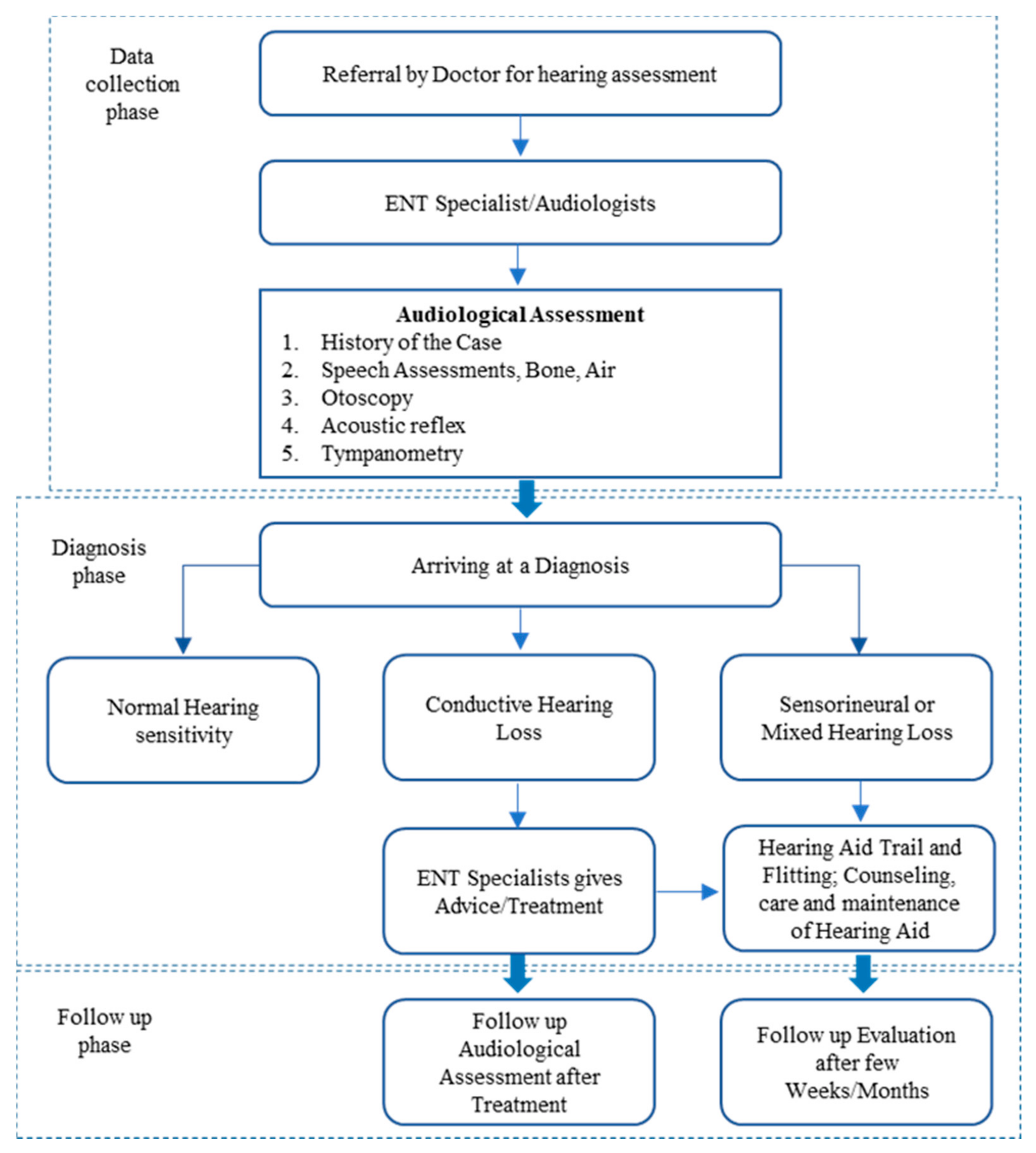
3.1. Proposed Identification Model

In this section, we introduce and discuss in detail our proposed detection model for hearing-loss symptoms. The model diagram shows the components of the proposed model and how each component processes the data. The NB algorithms and Frequent Pattern (FP Growth) were employed in the model as machine learning (ML) methods. A full description of those methods with the reasons behind employing them in the model is provided in this section. In healthcare literature [30,31,32], these methods are commonly used for similar illness and they were reasonably efficient and successful. This has motivated us to utilize these methods in our proposed model. In 
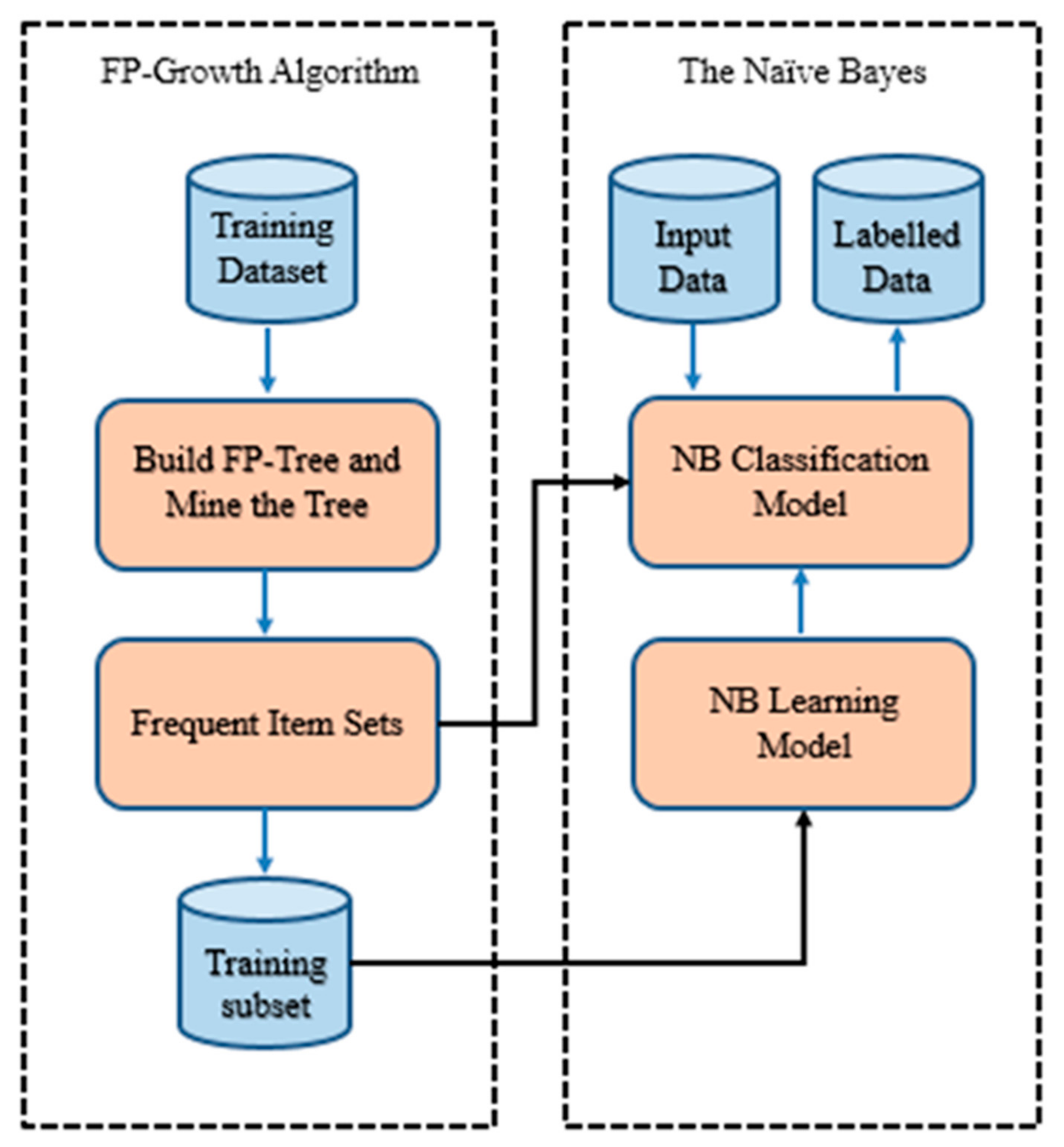
Figure 3, our proposed classification model for hearing-loss symptoms, and how the extracted data are frequently processed using the FP-Growth algorithm, is illustrated.
Each item set from the dataset reflect several features, each feature is a part of the vocabulary. In this model, the FP-Growth algorithm, utilized for processing the feature transformation after the process of selection and extraction of the feature, was conducted. The NB classification method was used for training a subset of frequent item sets that achieved the minimum support threshold, as shown in Figure 3. In this example, 242 training item sets out of total 399 training item sets achieved the minimum support threshold to be within the training set in the NB classifiers. Our model can minimize the data dimensionality and requirement repository for the classification methods. Besides, it can enhance the performance of the classification methods and eliminate redundancies. In a specific condition, the dimensionality of the whole training data is minimized and added to the training set for the classification method. Therefore, each training example should include some frequent features that achieve the minimum support threshold considered within the training set for the neural network classification method.
The requirement repository of the classification method is reduced in case frequent features are composed. This is opposite to the traditional method when consisting of the entire features of the training dataset. The common characteristics of the datasets are redundancies and noise. The redundancies can be removed when choosing one frequent item set in the data. It is obvious that the algorithm’s speed and performance can be increased once the dataset becomes small. In our proposed model, feature transformation advantages can be obtained, including construction, selection and extraction. New features can be created through all these feature transformation forms [33]. Functional mapping is used to extract new features from old ones [34]. The most important method in the dataset is a frequent feature extraction. Another important method in the dataset is a feature construction that generates additional features to replace the missing data. In this study, we employ the FP-Growth algorithm as linear and non-linear spaces to offer a feature construction process to minimize the data dimensionality and recovering the missing information [33]. Less data dimensionality makes the process easier and faster. However, feature selection can reduce the requirement repository and enhance the performance of the algorithm by removing the redundancies and noise [34].
An associative classification, which is a combination of unsupervised learning methods, such as the FP-Growth algorithm or association rule and NB classifiers, performs much better than the standalone classification method [35]. The hybrid of the FP-Growth algorithm and K-nearest neighbor (KNN) can obtain a high classification accuracy [36]. Our hearing loss detection model has utilized a combination of unsupervised and supervised learning ML methods, particularly the FP-Growth algorithm and NB classifier. The two versions of the naïve Bayes classification models, which are the multivariate Bernoulli and multinomial model, were explained. The multivariate Bernoulli naïve Bayes model was the model of choice for the classifier as the implementation with the FP-Growth algorithm has proven to be more efficient than the multinomial model. This is against the argument by other researchers that indicate that the multinomial model outperforms the multivariate Bernoulli in every respect, as depicted in the chapter using different kinds of datasets. The justifications for adopting these as the techniques for implementing the model are explained using various research in healthcare that uses a similar method with varying degree of success, as well as by the literature that support the efficiency of these techniques. The identification model for hearing-loss symptoms was depicted in a diagram and all the components that make up the model explained. The FP-Growth algorithm serves as a pre-processing mechanism that provides all the elements of data transformation to the data before it becomes part of the classifier’s vocabulary. With that, the advantages inherent in data extraction, selection and construction techniques were all achieved. These advantages include discarding redundant and noisy features in the data, reducing storage requirements and improving the classification algorithm’s performance.
The calculation of these parameters for the prior can be represented as follows:
From the union of all item sets that meets the minimum threshold, extract the vocabulary (V) for each class and get the training cases that have that class:
Calculate P( C j )terms
For each C j in C do
Training cases  t j ← All the training cases with class = C j
P C j = / t j / / T o t a l #   t r a i n i n g   c a s e s /
The algorithm shows the steps used to calculate the prior probability. The vocabulary of the classifier is extracted from the union of all the features in the item sets generated by the FP-Growth algorithm. Then, for every class of the training examples that qualifies to be in the training set, which in this case is the 242 training examples from the 399 in the dataset, calculate the probability of each particular class P(Cj) by getting all the training examples with class Cj among all the classes and divide it by the total number of all the training examples.
The calculation of these parameters for the multinomial likelihood can be represented as follows:
Calculate P( t k / C j )terms
Thresholdsj ← single set containing union of all frequent items sets (vocabulary)
For each t k in vocabulary
n k ← # of occurrence of t k in the training cases of class = C j
P t k / C j = / n k + α / / n + α \ v o c a b u l a r y /
The algorithm shows the steps for calculating the parameters for multinomial likelihood. To calculate the probability of a class given a particular training example.
P(tk/Cj), the vocabulary, is formed from the union of item sets of the thresholds. Then the number of occurrences of the threshold tk in the training examples of class Cj is calculated plus the alpha (α) divided by the total number of tokens (n) in class Cj plus additive smoothing alpha (α).
The calculation of these parameters for the multivariate Bernoulli likelihood can be represented as follows:
Calculate P( d k / C j )terms
Thresholdsj ← single set containing union of all frequent items sets (vocabulary)
For each t k in vocabulary
n k ← # of training cases where t k is present
P d k / C j = n k + α n + α \ v o c a b u l a r y
The algorithm shows the steps for calculating the parameters for the multivariate Bernoulli likelihood. To calculate the probability of a class given a particular training example P d k / C j , the number of training examples nk where the threshold t k is present is added to the smoothing parameter alpha (α) and divided by total number of tokens plus the alpha (α).

3.2. Identifying the Relationship with Association Analysis Algorithms

Unsupervised learning methods, such as association analysis algorithms, have the capability to find a correlation with invisible datasets [37]. Frequent features (item sets) and association rules can be found using this method as discovered segments. If there is a strong relationship between more than two item sets in the dataset, then this is a suggestion of an association rule, which is represented by A → B, where A and B are distinct item sets. The support and confidence metrics are used to measure the correlation of the item set elements in a dataset. Support metric reflects the frequent number of a rule that is used in the dataset at hand. ADi audiology data compresses the S item set where S is a subset of ADi, mathematically formulated as follows:
σ S = | { A D i | S A D i , A D i D } |
σ(S) represents support for an itemset S. ADi represents individual audiology data with S as its subset (SADi). This is means that each item of S is can be an item in ADi, where ADi is also an element of the dataset (D). A confidence metric is used to measure the interface reliability of an association rule. It suggests a strong correlation between items within an itemset in the preceding and succession of the rule. In instance, the rule TNTS → 2000:30 shows a big confidence value with a big probability hearing threshold between 2000 and 30 in the individual audiology data ADi that included TNTS. The confidence metric reflects the frequency of a number of elements in the S itemset in ADi data that compress the T item. The Confidence and Support measurements can be formulated as follows:
S u p p o r t S = e s / N A D i
C o n f i d e n c e S     T = e s T / e s
The combination of the FP-Growth algorithm and association analysis is powerful and have a capability of item extraction from the dataset [38]. The FP-Growth algorithm is used to generate a frequent itemset within a dataset for patients with hearing loss. The FP-Growth algorithm represents the dataset in a tree data structure known as the FP-tree. Each FP-tree has a path that maps to certain training example after it is scanned by the FP-Growth algorithm [39]. Different features can be reflected by various training examples. The deep interference of the structure of the FP-tree leads to better dataset compression for the FP-tree. 
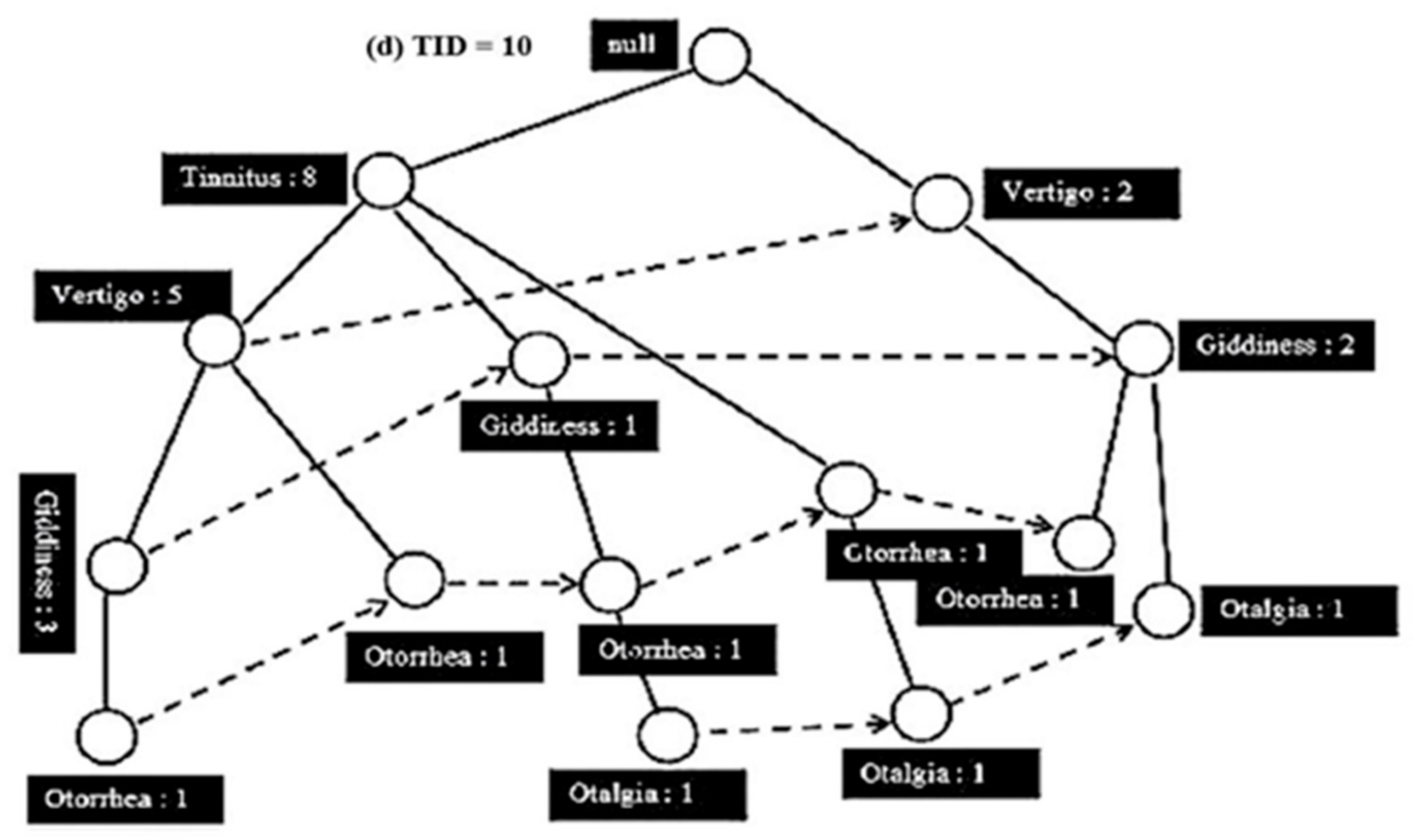
Table 2 illustrate the structure of the dataset in details.
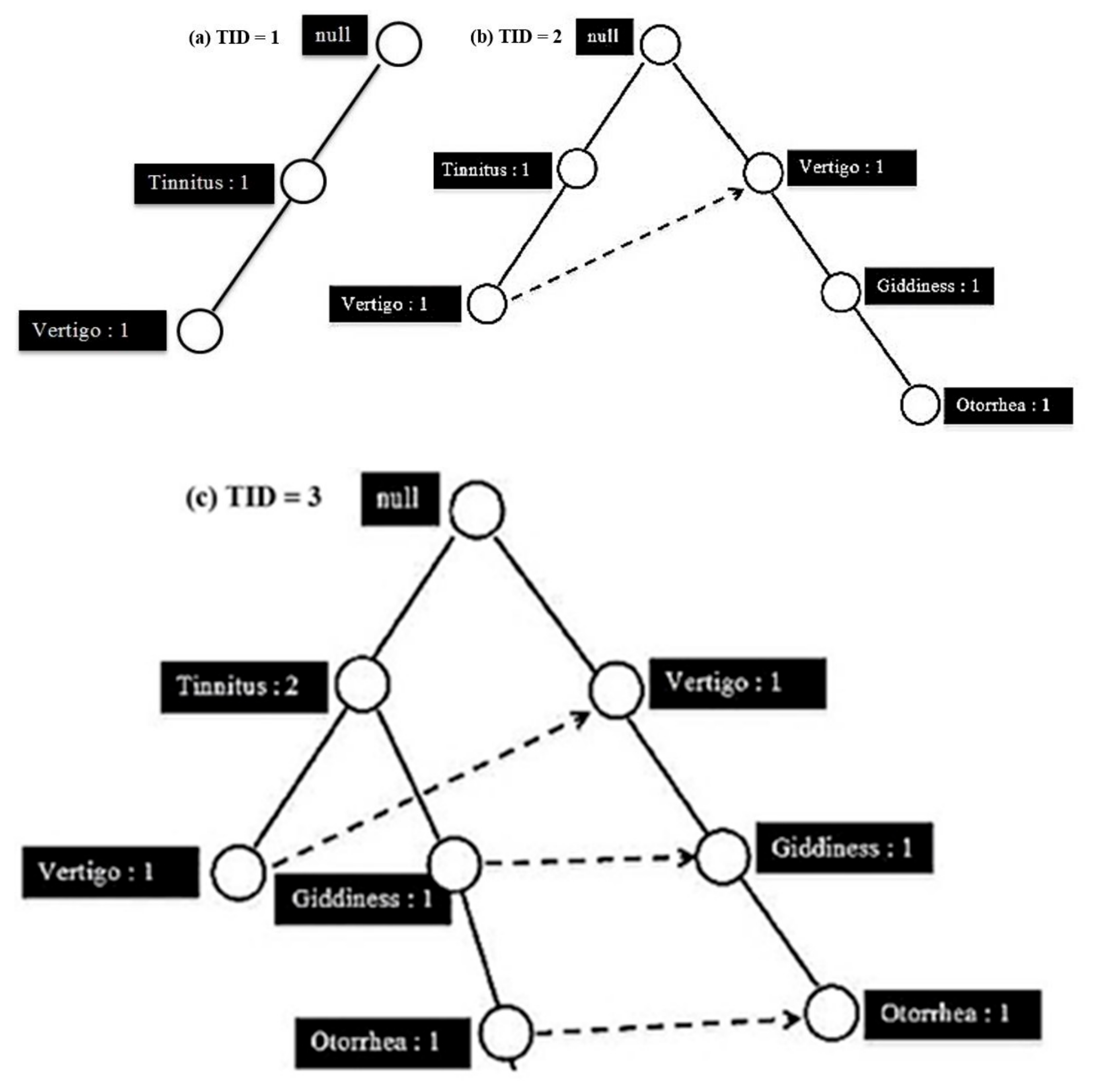
Figure 4 illustrates the FP-tree structure of the dataset where each consists of five features and ten training examples, including (a) TID 1, (b) TID 2, (c) TID 3 and (d) TID 10.
In the FP-tree, for each given path, each node represents a feature with a counter for the training example number that is mapped to this path. In the FP-tree, null is the root node, representing the starting point of the FP-tree. Firstly, the FP-Growth algorithm scans the number of frequencies for each item in the dataset and then it removes the item with no frequency count. Thus, an infrequent item leads to infrequency as well. Then the FP-Growth algorithm rescans the number of frequencies to build the structure of FP-tree to extract the frequent item sets [40]. For example, tinnitus is the most frequent item set in our dataset, followed by vertigo and then giddiness, otorrhea and lastly otalgia. After the FP-Growth algorithm generates an FP-tree structure, it crosses the first training example to generate the nodes as Tinnitus → Vertigo. Initially, the FP-tree start from the null node then the other path will be created by the training example as null → Tinnitus → Vertigo. In the example, each node in this path has a frequency count equal to 1. In the second training example, another path will be created from nodes the Vertigo, Vertigo, Giddiness and Otorrhea as null → Vertigo → Giddiness → Otorrhea. The second path is created due to there being no overlap with the first training example that represents the first feature (tinnitus). However, in the third training example, there is an overlap with the first training example in the first feature (tinnitus). So, for the path of null → Tinnitus → Giddiness → Otorrhea → Otalgia, the count feature (tinnitus) becomes two as it is overlapping with the third training example.
FP-Growth algorithm repeats this process until to reach the tenth training example. In addition, frequent item sets are generated by the FP-Growth algorithm to build a conditional branch of FP-tree in a bottom–top approach. The FP-Growth algorithm finds the frequent item sets ending with otalgia, and then it looks for another itemset that ends with otorrhea, giddiness, vertigo and tinnitus. This process is reasonable as each branch in the FB-tree is mapped to each training example. Therefore, for a given feature, a path is traversing to generate frequent item sets. We used settings 0.1 and 0.7 for the minimum support threshold and confidence thresholds, respectively, on the sample audiology dataset of 50 patients. Furthermore, we used settings of 0.2 and 0.7 for the minimum support threshold and confidence thresholds, respectively, on the sample audiology dataset of 339 patients. It is hard to find lower values for the minimum support and confidence threshold measurements. Therefore, we chose 0.2 (20%) and 0.7 (70%) for the minimum support and confidence threshold values as it could achieve the result at an acceptable level. Setting the values to less than 0.1 (10%) of the dataset leads to an undesired result.

3.3. Feature Transformation with FP-Growth Algorithm

The FP-Growth algorithm was applied on an audiometry dataset of 399 patients using air and bone conduction audiology medical records. The FP-Growth algorithm acts as a frequent item set extraction algorithm with a setting of 0.4 (40%), the minimum support threshold. Each item set in the training examples that pass the minimum threshold is integrated into the training set for the NB as a classification method. Opposite to the traditional method, which extracts the vocabulary form of all item sets (features) in the training examples, the NB extracts the item sets from a union set of item sets. Only 242 out of 399 training examples were found after the process of the item set generation. Those training examples do not belong to their subset of the generated item sets. Only three symptom types were found from the extracted item sets. From 242 training examples, there are tinnitus symptoms and some symptoms of both tinnitus and vertigo and other symptoms with tinnitus, vertigo and giddiness. The FP-Growth algorithm is fed by the neural network by three labels to identify the symptom of the air and bone conduction audiometry. The first label is tinnitus, the second label is tinnitus and vertigo and the third label a collection of tinnitus, giddiness and vertigo. The air and bone conduction thresholds could consist of undesired frequent aspects for the same frequency or decibel for hearing in both ears of the patient. This can lead to increasing the dataset and features’ dimensionality and resulting in noisy features. The FP-Growth algorithm extracts features patterns to build up the classification vocabulary. New features can be created by one of the common feature transformations, such as feature construction, selection and extraction [41]. The feature extraction method is used to extract the frequent item sets from the dataset. The feature construction method is a pre-processing method used to reduce the dataset dimensionality. It is a very critical method as the success of machine learning approaches depends on this process. The feature selection method is used to select features from the dataset to reduce the requirements repository and enhance the performance of the classification algorithm [42].
In this study, we employed all three feature transformation techniques. Extracted item sets (features) were used to build up the vocabulary. This leads to minimizing the feature number for vocabulary. Thus, this minimizes the feature dimensionality as well, which helps the vocabulary keeping the relevant data. The vocabulary consists of a number of disjoint item sets (features) in the training examples [43]. Thus, the three feature transformations, extraction, selection and construction, are attained. Reducing the requirements repository, removing the noisy feature and lowering the computational complexity result in enhancing the performance of the classification algorithm, and a lower feature number means higher speed processing. Factor analysis, independent component analysis and principal component are the most common techniques used to reduce the feature dimensionality [44]. In this research, we employ the FP-Growth algorithm in our detection model to offer a feature construction process to minimize the data dimensionality and recovering the missing information [45].

3.4. Patterns Evaluation

A large number of item sets and form patterns can be generated by the FP-Growth algorithm within the minimum support threshold. The FP-Growth algorithm tends to generate a huge number of patterns since the size of the dataset is very big. The issue is that some of these generated patterns are undesirable. It is not a trivial process to identify the desirable patterns and undesirable ones as this decision depends on many aspects. Thus, using standard evaluation methods for pattern quality is a necessity. Statistical methods are one of these methods used to evaluate the quality of the generated patterns [46]. It can be considered that the item sets that have a lower number of items or are discovered in less of the training examples are undesirable item sets. An objective interestingness metric can be used to remove these item sets. An objective interestingness metric is based on statistical analysis that identifies which item set should be removed. In the literature, several objective interestingness metrics is proposed to discover the desirable item sets concerning specific aspects. An aggregating method is proposed in [47] to discover the desirable association rules using an advanced aggregator. The ranking method comprises two processes. The first process is based on the chi-square test technique while the second process is measuring the objective interestingness. Objective interestingness measurement is commonly used in the literature. It relies on the relationship of the confidence threshold and minimum support threshold [48].
A study on the objective interestingness measurement was conducted by [49], demonstrating that some interestingness measurements can reduce the association rules number efficiently. However, the accuracy quality is not improved. In addition, no individual interestingness metric is superior to others. Another standard evaluation method in the evaluation of desirable item set quality is subjective arguments. In this method, the itemset can be desired if it offers unpredicted beneficial information for the discovered data. In this study, we employed subjective knowledge arguments as an evaluation method. This is because of the advanced knowledge obtained from the patients’ medical audiology data. The template-based method is employed as a subjective knowledge evaluator to evaluate the extracted item set quality. Thus, the generated item set using the FP-Growth algorithm is allowed to be restricted as all the items are filtered, keeping only the itemset that has one or more symptoms, such as vertigo, tinnitus, otalgia, Meniere, and others. In this paper, the template-based method is used because of its advantages that has been demonstrated in many recent studies. Besides, it can enhance the search of keywords using semantic data [50]. Researchers and scientists who are experts in this domain can only use their knowledge and experience to discover the important patterns. So, the patterns selected by the expert template only were extracted.

3.5. Symptoms Identification with the Naïve Bayes Algorithm

We performed the classification process on the output of the training set obtained from the recurrent item sets when applied on the FP-growth algorithm. We used two common methods of naïve Bayes, including a multinomial model [17] and multivariate Bernoulli, to find out the most accurate solution. The naïve Bayes method is applied to the hearing loss classification problem to detect the symptoms for the thresholds of bone conduction audiology and the pure-tone air. In the multivariate Bernoulli method, the vocabulary and a training example act as inputs, after which they are processed to obtain the binary output classification. The binary classification can be represented by a vector of ones to reflect the condition of the existing hearing threshold while it can be represented by a vector of zeros to reflect the condition of the absence hearing threshold. The vocabulary consists of several different features that form the training examples [18]. The vocabulary length binary should be the same length as the binary vector. The vocabulary results contain various features and thresholds. For a given class, the multinomial model produces the portion of times that the threshold values of the training examples appear. In our proposed model, the threshold value of the frequent item set is insignificant compared to the threshold value state, whether in existence or absent in the training example. Therefore, we employed the multivariate Bernoulli for this purpose. The training example was divided into a number of feature sets to extract the features, including the bone conduction audiology thresholds and symbols of air from the dataset. The threshold of audiology hearing reflects the given frequency level and decibel at the point of hearing the pure tone. A vector of ones and zeros symbols represent every training example. A one value indicates that the symbols are available in the training example while the zero values indicate that the symbols are unavailable the training example. The estimated training examples of the probabilities and conditional probabilities for the given class feature were used to train the classification methods [19]. The naïve Bays process is formulated in the mathematical equations as follows:
The Bayes rule is formulated as in [17,20]:
P ( C | D ) = ( P ( D | C ) P C ) / P D
This is applied in the classification method and formulated as
C _ m a p = a r g m a x   P C / D   c C
C_map represents the best class, which is the one excluded from all classes that maximize the values argmax and P(C/D). Using the Bayes rule, every class is maximized by Equations (4) and (5):
C _ m a p = P D / C   P C   c C
The class that could maximize the product of P(D/C) P(C) is most likely to be selected. The goal is selecting the class that is associated with the probability bigger than the specific audiology thresholds that have the symptom or set of symptoms.
Equation (6) can be reformulated as
C _ m a p = a r g m a x   P x _ 1 , x _ 2 , x _ 3 x _ n / C P C   c C
The common probability of x_1 via xn conditioned on a class can be symbolized as the product of independent probabilities P x _ 1 / C   P x _ 2 / C   P x _ 3 / C . .   P x _ n / C .
To calculate the most likely class, the probability of the initial of likelihood features is multiplied by the class probability. This can be reformulated as
C _ N B = a r g m a x   P C _ j P x / C _ j   c C   x X
C_NB is the best class that maximizes the advance class probability P(Cj) multiplied by each probability of the feature in the given feature class. In the data, for each hearing threshold position in the given class probability, the class is computed and assigned the best probability. The frequent item sets in the data were computed for classification training purposes.
For the advance training example (t) that is available in a class (Cj), the number of training examples in class (Cj) was divided by all training examples counted, as represented by the following equation:
P ^ ^   C _ j = t c o u n t c = C j / N t
In in multinomial model, the likelihood and the threshold probability i (ti) for the given class (Cj) can be calculated by the number of times the threshold of i (ti) is counted for the given class (Cj) in the training example and then dividing it by the overall threshold number across all training examples of class (Cj), as represented in the following equation:
P ^ ^   ( t i | C j ) =   c o u n t t i , C j / c o u n t t , C j   W V
The portion of training examples of class (Cj) of the appeared threshold in the multivariate Bernoulli method is divided by the overall training examples number in class (Cj), as represented in the following equation:
P ^ ^   ( d i | C j ) =   c o u n t d i , C j / c o u n t d , C j   W V

4. Results

This section discusses the first and second experimental results of the study that is aimed at finding a relationship between the audiometry thresholds and attributes in hearing-loss patient medical records, using association analysis. The section also presents the results of the implementation of the identification for hearing-loss symptoms using the FP-Growth feature transformation and the performance of the two naïve Bayes classification models; multivariate Bernoulli and multinomial models with and without the FP-growth feature transformation technique. The reason why the multivariate Bernoulli naïve classifier model is adopted for the implementation of the proposed model is also explained in this section.

4.1. Dataset Used

The National Medical Research Register (NMRR) in Malaysia is considered the official data bank in the medical field. Researchers can register their medical research online at NMRR for review and get approval for sample data collection by the concerned authorities. Our research has obtained NMRR registration and sample data collection approval. The type of data used for this research is secondary data. The type of secondary data collected for the research is the medical records of hearing-loss patients, including their audiometry data. This type of data is typically recorded by the audiologist and otolaryngology specialists in the course of diagnosing the patient during consultation. A collection of the audiometric data from the period between 2003 and 2012 were obtained from an otolaryngology department in a Malaysian local hospital. The collection data belonged to 399 patients with hearing difficulties aged from 3 to 88 years old. The data collection ranged from 0.125 kHz to 8 kHz for 11 frequencies measurements. To find out the link between the symptoms of hearing loss and audiometry threshold of pure-tone air conduction, a Frequent Pattern Growth algorithm (FP-Growth) combined with rule mining algorithm were used on a sample dataset of 50 patients with hearing difficulties with a setting of 0.7 and 0.1 for the confidence thresholds and the support threshold, respectively. The FP-Growth and rule mining algorithm were also employed on another bigger sample dataset of 399 patients with hearing difficulties with the setting of 0.7 and 0.2 for the confidence thresholds and the minimum support of the item set generation, respectively. Both studies reveal that there is a correlation between the audiometry thresholds and the symptoms of hearing loss, such as dizziness, vertigo, tinnitus and other medical information.
The small dataset: FP-Growth algorithm combined with the rule algorithm were employed to find the correlation of audiometric configuration and the characteristic of patients with hearing difficulties on a sample of pure-tone air conduction audiometry data, collected from 50 medical records of patients with hearing loss. The hearing loss characteristics included data structures of age, gender and symptoms. The confidence thresholds were set to 0.7 and the minimum support was 0.1, as the association rule that set to 0.1 (10% of the dataset) or more is more motivated than an association rule that is set to less than 10% of the dataset. The dataset included a collection of data of pure-tone audiometry thresholds and the characteristic of hearing loss from medical records. Around 349 frequent item sets were generated using the FP-Growth algorithm based on the association rules mentioned above.
Large sample dataset: Using the same method, the experiment is repeated on the entire dataset that contains data of 399 hearing-loss patients, including the sample data that applied in the initial experiment. The value of the confidence thresholds has not changed, which is equal to 0.7, while the value of the minimum support is increased to 0.2.

4.2. Data Preparation

We prepared the dataset in a way that is easier for the algorithm to read and apply it. Discrete data are more likely to be chosen because of the sorting way of the item sets. Some symptoms of the hearing loss were abbreviated, including vertigo as (VTG) and tinnitus (TNTS), while other symptoms were not abbreviated, including rhinitis, prescubysis, otalgia, giddiness and otorrhea. The patient’s characteristics and attributes also were abbreviated, including gender represented male as (M) and female as (F). The patient’s age was abbreviated as early (E), mid (M) and (L) late. For instance, 5 M (the mid 50 s) is representing a male of 55 years old and 8 L (the late 80 s) is representing a male of 89 years old. We used a colon (:) in the hearing thresholds as a separator between the sound frequencies and the sound dB. For instance, hearing thresholds of 500:45 R represent a 500 Hz frequency and 45 sound dB for the right ear, while 8000:80 L represents 80,000 Hz frequency and 80 sound dB for the left ear. In another study [30], symptoms of hearing loss, attributes and structured data, such as date of birth, gender, type of hearing device and other medical information, were abbreviated and applied on statistical and neural methods for patients classification to help in selecting the most beneficial hearing device for the appropriate patients. It is necessary to change the data format to be acceptable for the given algorithm.

4.3. Performance Evaluation and Validation

The error rate metric was used to measure the performance of our detection model. To calculate the error rate, a cross-validation technique was applied, and the random sub-sampling validation method was used to repeatedly divide the dataset into two sets: one used for the training while the other used for the validation. To validate our model, a validation technique was applied to randomly divide the dataset to obtain training and test sets during the execution time. The validation technique was iteratively repeated ten times and then the average error rate was computed. For each training example, this method was applied to select the sets for the test and training. Each grouped training example was chosen randomly after was divided at each iteration. The errors rate was averaged after a number of iterations for each partition group. It suggested applying the NB on the dataset prior to the pre-processing step to make a performance comparison using a different representation. It also suggested taking the risk of using the whole information and data rather than the risk of reduced information. Our model was implemented by the Python programming language. The testing also was conducted in the same programming language. Python was chosen as it is a powerful and efficient programming language for mathematical computation [51,52,53,54]. Otorhinolaryngology specialists are involved in the validation process in the first and second experiments for the results confirmation purpose. These experiments were based on the extracted patterns that reflect the correlation of the audiology thresholds and symptoms of hearing-loss symptoms.

4.4. Results from the Association Analysis Using the Small Sample Dataset

The pure-tone air conduction audiometry data for 50 hearing-loss patients were collected to find any possible connection between the audiogram configuration and attributes in the hearing-loss patients’ medical records. These attributes consist of structured data, such as symptoms, gender and age. The FP-Growth algorithm and association rule algorithm was used for this purpose. The minimum support for item set generation was set to 10% (0.1) and the minimum confidence for the association rule was set to 70% (0.7). The dataset comprised pure-tone audiometry threshold data in a combined form with additional characteristics as found in the medical records. The FP-Growth algorithm generates 349 frequent item sets from which association rules are generated. The results of some association rules are interesting, of which 93 are depicted in the exact format of the output of the FP-Growth and association rule algorithm (Table 3, Table 4 and Table 5). Moreover, the association rules are further summarized in Table 6, Table 7 and Table 8.
These rules show the hidden relationships in the small sample dataset (50 cases) using 0.1 (10%) as the minimum support threshold. The confidence in the rightmost column is used to measure the strength of association between items in the dataset. From the item sets above, the association rule (TNTS → 2000:30 R, F) denotes a strong correlation between the symptoms of tinnitus (TNTS) with a 2000:30 hearing threshold in the right (R) ear among females (F) in the sample dataset of 50 hearing-loss patients. Table 7 provides the summary and meaning of the abbreviations in Table 3. 2000:30 R is a threshold at the frequency of 2000 Hz at sound decibel of 30 dB. The confidence thresholds on both tables mean the percentage of the training examples in the dataset containing a given rule. For example, a 1.000 confidence in the rule (TNTS → 2000:30 R, F) means that, in 100% of the training examples in the dataset containing TNTS (Tinnitus), the rule is correct.
The result (TNTS → 500:55 L, 250:60 L) means a strong relationship between tinnitus and the hearing threshold at a mid-frequency of 500 Hz and 55 dB (sound decibel). This rule also shows a possible tinnitus connection with 250 Hz (low frequency) at 60 dB, all in the left (L) ear. The other generated association rules in the table also show interesting relationships between tinnitus and hearing thresholds and other attributes in the dataset. According to evidence from other researchers, flat, cochlear-type hearing impairment can be detected on the audiogram of tinnitus patients and that low frequencies are most affected. In addition, the shape of the audiogram is often flat or rising but any configuration is possible. From the results, a low frequency of 250 Hz can be seen. Moreover, as evidenced by the literature, the shape of the audiogram is often flat; that is, the hearing thresholds are mostly at lower sound decibels but at various frequencies. Table 7 shows a summary of all the discovered rules.
Table 5 shows the association rules for vertigo. One of the symptoms of hearing loss diagnosed in patients is vertigo. The level of confidence met by the item sets depicts an interesting relationship between vertigo and hearing threshold and other attributes. The rule (VTG → 1000:10 L, 500:20 L) denotes the probability that vertigo patients experience hearing loss from a mid (500 Hz) to high (1000 kHz) frequency at lower sound decibels (10–20 dB) in the left ear. Looking at the whole association rules, it can be observed that, bilaterally, there is a relationship between normal hearing (NH) and vertigo, depicting a mid to high frequency (1000 kHz, 2000 kHz and 4000 kHz) for normal hearing. The rule (VTG → 4000:65 L, F) denotes a possibility of females having hearing loss with an extreme frequency of 4000 kHz at 65 dB given that vertigo exists. Table 6 shows the summary of all the discovered rules in Table 5, which includes the symptom of vertigo and some hearing thresholds.
Table 4 shows the association rules within the item sets consisting of vertigo together with tinnitus. A correlation between the vertigo and tinnitus and hearing threshold values are shown by all the rules. As evidenced by other studies, vertigo and tinnitus can also occur together [55]. Table 8 shows a summary of all the discovered rules in Table 5 that includes the symptom of tinnitus and vertigo and some hearing thresholds.
Table 9 depicts the relationship between giddiness and the hearing threshold inside the right ear occurring at a low frequency and low sound decibels in females (GIDDINESS → 250:35, F). The other rule (TNTS, GIDDINESS → 250:35 R, F) shows a similar interesting relationship between giddiness, tinnitus and a low-frequency threshold among females. Table 10 shows the summary of all the discovered rules in Table 9, which includes the symptom of giddiness and some hearing thresholds.

4.5. Results from Association Analysis Using Large Sample Dataset

Table 3, Table 4 and Table 5 and Table 9 present the pure-tone audiometry measures obtained from the dataset of 50 patients involved in a primary study [56]. Correspondingly, Table 11 and Table 12 compare the previous results with that of an air and bone conduction audiometry data carried out on 339 patients. The study by [56] stated that from the dataset of the primary study involving 50 patients with hearing loss, it was gathered that a correlation exists between audiometry thresholds, gender and hearing-loss symptoms. Furthermore, each of Table 13 and Table 14 presented results from Table 11 and Table 12.
The outcome of the primary research on the 50-patient dataset and pure-tone audiometry processes are illustrated in Table 3, Table 4 and Table 5 and Table 9. A comparison with the outcome for the research on 339 patients’ air and bone conduction audiometry data is in Table 11 and Table 12 below. There is a connection between the hearing-loss symptoms, gender and audiometry thresholds from an initial study on a dataset of 50 hearing-loss patients [26]. The tinnitus was represented as TNTS, vertigo as VTG, normal hearing as NH, BILATERAL referred to the two ears, M referred to male while F referred to female, L represented left ear while R represented right ear. The support value for itemset generation was set at 0.1 (10%) while the confidence value for the association rule was set at 0.7 (70%). The correlations between pure-tone audiometry thresholds and vertigo, tinnitus and giddiness were an interesting discovery.
Table 11 and Table 12 present the results of the current study on association rules. The comparison between Table 3 (observed tinnitus association rules) and Table 11 (the latest observed results of tinnitus and vertigo association rules) reveals the correlation between tinnitus symptoms and normal hearing threshold occurring at 500 Hz (500:15 R, → ONOFF TNTS) inside the right ear—R‖, as presented in Table 3. Table 11 presents the reflection of this in the results of the current study involving 339 patients depicting a relationship between tinnitus symptoms and vertigo and normal hearing threshold occurring at 500 Hz (TNTS, VTG → 500:20 R, M) in male patients’ right ears—RI. Akin to this kind of relationship is that seen between the normal hearing threshold and vertigo (VTG, M → 500:20 R, NH, BILATERAL) and (VTG → 500:15 R, F) in Table 3 for the initially observed vertigo association rule. Table 11 presents the results of the association rules (TNTS, VTG → 250:40 R, 400:45 R, F). These rules can be likened to those observed in the primary study as depicted by Table 3 (TNTS → 250:30 R, F), (TNTS, M → 250:60 L) and (TNTS → GIDDINESS, 250:35 R, F). A close look at both studies (the primary study and second study) shows some similarities, as seen in the low-frequency, mild–moderate hearing loss in patients with the tinnitus condition. Table 5 depicts a reflection of the results (250:35 R → VRTG, F).
The correlation between giddiness symptoms and pure-tone thresholds is presented in Table 12. This signifies a correlation between giddiness and hearing normal at high-frequency thresholds inside the left ear and right ear (GIDDINESS → 1000:10 L, 500:20 L, 250:25 R). A related result is reflected in the primary study presented in Table 9 (500:20 R → GIDDINESS). Table 13 and Table 14 shows the summary of all the discovered rules in Table 11 and Table 12, respectively, including the symptom of tinnitus/vertigo, giddiness and some hearing thresholds.

4.6. Symptoms Prediction and Model Evaluation

The significance of the feature extraction methods cannot be overemphasized. It is significant in the accomplishment of many AI methods [56]. The exhibitions of the classifiers utilizing both multivariate Bernoulli and multinomial models with and without features extraction were compared. Our study displays the validation outcomes of the machine learning assessment used in the dataset with 242 training samples. The validation outcomes utilizing the multivariate Bernoulli model (MVB-FPG) with FP-Growth feature transformation appear in Figure 5. Also, further details have provided in Table 15.
Figure 6 display the 10 iterations utilizing 5 unique segments of the cross-approval method with the average error rate (Repeated Random Sub-Sampling Validation Technique), a technique that is used to test the accuracy of a classifier. Using 10 training samples, there is a 100% expectation of exactness utilizing allotment; also, the ratio can be predicated as 99.5% precision with 20 training samples; in addition, 99% with 30 training samples, 98.25% with 40 training samples and 94.60% prediction with 50 training samples. Therefore, the average error rates for the five distinct segments were 0, 0.5, 1, 1.75 and 5.4%, respectively. The ML method work astoundingly with the multivariate Bernoulli model (MVB) with FP-Growth features processing.
Figure 7 illustrates the validation outcomes above 10 iterations utilizing diverse segments. The assessment acquired from the multivariate Bernoulli model without FP-Growth features processing differs from the outcomes acquired with FP-Growth features processing. Figure 6 displays the average error rates utilizing the multivariate Bernoulli approach without the features processing. The average error rate for every segment is a high ratio. The segments with 50 and 40 training samples have the worst average identification incorrectness with a 57% and 56% average error rates, respectively. The segments with 10, 20 and 30 training samples have up to 50% error rates. Table 16 shows the summary of all the percentage error and accuracy rate of the multivariate Bernoulli naïve Bayes classifier (MN-FPG) model without FP-Growth feature transformation.
Figure 8 shows that the average error rates rely on 10 iterations utilizing the 5 diverse segments of the validation group, and the outcome of the multinomial NB method with FP-Growth features processing. The segment with 50 training samples have achieved the best, with 10% error rates averaged over 10 iterations task. Therefore, the identification rates were precisely 90%. While, the minimum average error rates were 2%, which is for the segment with 10 training samples. It can be concluded to use average error rates of 3%, 3.9% and 8.5% for 20, 30 and 40 segments, respectively. Table 17 shows the summary of all the percentage error and accuracy rates of the multinomial naïve Bayes classifier (MN-FPG) model with FP-Growth feature transformation.
Figure 8 displays the validation outcomes utilizing the multinomial model without FP-Growth features processing. The segment with 10 training samples have acquired the minimum average error rate of 42%. While, the maximum value for a segment with 20 training samples achieving a 53% average error rate. The segments with 30, 40 and 50 training samples got error rates of 48%. All the error rates are averaged above 10 iterations. Table 18 shows the summary of all the percentage error and accuracy rates of the multinomial naïve Bayes classifier model without FP-Growth feature transformation. According to Table 15, Table 16, Table 17 and Table 18, the results indicated that a low average (AV) error rate and high average (AV) accuracy for the proposed models are achieved only when adopting the FP-Growth feature transformation.

4.7. Discussion

The results of this study indicate a possible connection between patients’ audiogram configuration and some attributes in their medical records. These attributes include age, gender, symptoms, medical history, etc., as evidenced in other studies stated in Section 2 of this study. This experiment has detected evidence of the relationship between the patient’s audiogram configuration and hearing-loss symptoms when experimenting with both a small sample dataset of 50 hearing-loss patients and a larger dataset of 399 patients. The initial study using a smaller sample dataset found a relationship among tinnitus symptoms, vertigo symptoms, giddiness symptoms and hearing thresholds at different frequencies and sound levels. These include some attributes such as age and gender in the relationship. The most interesting findings were that the results of the first experiment with the smaller data sample correlate with the results of the second experiment with a larger dataset sample of 399 hearing-loss patients. For example, the results in the second experiment show the symptoms of tinnitus and vertigo to be related with mild hearing loss at lower frequencies in females (TNTS, VTG → 250:40 R, 400:45 R, F). There were similar results seen in the first experiment in Table 1 where the symptoms of tinnitus is related to mild hearing loss at a low frequency (TNTS → 250:30 R, F), (TNTS, M → 250:60 L) and (TNTS → GIDDINESS, 250:35 R, F). This implies that a huge similarity exists between the two results since low-frequency, mild–moderate hearing loss exists among tinnitus patients in both results. The same was found in the case of symptoms of vertigo. The result is in Table 3 (250:35 R, VTG → 500:25, F), and 250:35 R → VRTG, F is also reflected in Table 5 (250:35 R → VRTG, F).
A significant result was the correlation of the input data used in the Bayesian classifier and the high accuracy of predicting hearing-loss symptoms. It shows that the prediction accuracy is becoming high when the vocabulary of the classification method consists of item sets with a high frequency. The comparison results show that the multivariate Bernoulli method is superior to the multinomial method alone or even when combined with the FP-Growth feature transformation technique in terms of the prediction accuracy. The multivariate Bernoulli method integrated with the FP-Growth algorithm obtains a 5.4% average error rate on 50 training examples for ten iterations for random sub-sampling. The multinomial method with FP-Growth obtains a 10% average error rate on the same number of training examples and iterations. As the testing and validation process that used a big number of random training examples yields a better accurate result and more reliable model, we prefer to use 50 partitioned training examples. The experiment results demonstrate that both the multinomial and multivariate Bernoulli method with no FP-Growth combination perform badly in a partition with 50 training examples and yields the biggest average error rates of 48% and 57%, respectively. The absence of a feature transformation technique affect the performance of both methods negatively with this size of the dataset. It is surprising to note that the average error rates for both methods without the feature transformation technique are high in all five partitions at the tenth iteration. In addition, the average error rate of the multivariate Bernoulli is quite higher compared to the multinomial method. These findings support the outcome of another study in [4], which demonstrate the multinomial method is superior to the multivariate Bernoulli method on four diverse datasets. Other findings show that the multinomial method is superior to the other four probabilistic methods, including the multivariate Bernoulli methods on three text classification problems. Despite these findings, the multivariate Bernoulli method is superior to the multinomial method when combined with the FP-Growth algorithm. The average error rate of the multivariate Bernoulli method is smaller than the multinomial method when both combined with the FP-Growth algorithm in the five partitions. However, these outcomes are in contrast to findings in [4], which indicates the multinomial method performs better than the multivariate Bernoulli with respect to the prediction accuracy because of the number of word frequency. In [4], an argument was based on the vocabulary size, as the multinomial method yields better results on the smaller size while the multivariate Bernoulli method yields better results on the bigger size [4].
However, a contradiction to this argument is in [57], as it shows that the word information size does not affect the performance of both methods and the multinomial method is superior to multivariate Bernoulli method regardless of the information count. Moreover, the author of [57] argues that minimization of the word information count lead to improvement in classifier performance. Despite all previous studies that reinforced the multinomial classifier, our study demonstrates that the multivariate Bernoulli method is better than the multinomial method when the vocabulary formation includes frequent item sets of subsets that belongs to every training example in our dataset.
According to the SD analysis in Figure 9, overall we found that MVB-FBG and MN-FPG have scored highest and almost the same values in all training and validation data splitting approaches; this confirms the stability of the classification performance (accuracy) of the proposed models.
As shown in Figure 10, of the analysis of the error rate, we found that MVB-FBG and MN-FPG have scored the lowest and almost the same values in all training and validation data splitting approaches; this confirms the stability of with a low error rate performance (misclassification) for the proposed models.
However, we performed the Wilcoxon signed-rank statistical test [58] to verify, on the one hand, whether a significant difference exists between MVB-FPG and MVB. On the other hand, whether there is a difference between MN-FPG and MN. Error rate and accuracy values for all classifiers with five training sets were the main input for the Wilcoxon signed-rank statistical test, as shown in Table 19.
In the Wilcoxon signed-rank statistical test the main indicator is T-sig. The result is significant when T-sig < 0.05. According to the Table 19, all of the tested results are significant and satisfied the Wilcoxon test.

5. Limitations of the Study

This study is not without constraints and limitations. The size of the sample dataset available for the research is a limitation that cannot be overlooked. The accuracy of the prediction from a large dataset better shows the efficiency of the algorithm than the accuracy of prediction from a mid-range or small dataset. It is believed the higher the amount of training sets and validation data available for machine learning algorithms, the more reliable the classification or prediction result will be. This limitation is due to the fact that a lot of patient data collected from the Department of Ear, Nose and Throat at Hospital Pakar Sultanah Fatimah, Muar, was without an audiogram. This is because some of the patients were diagnosed with either nose or throat disease. Thus, this does not require any hearing measurement. Another constraint is the format in which the collected data comes with. The data collected is in paper format; therefore, there is the need to convert it into a digital format. This has become tedious work because each and every air and bone conduction hearing threshold value has to be recorded with the corresponding patient data. One of the drawbacks of using a small dataset is that not all training examples in a small dataset can have an itemset as a subset that pass the minimum support value. This can result in the exclusion of those training examples from those that will be chosen as the training set, as seen in this study where only 242 were chosen out of the 399 training examples in the dataset. In the case of a very large dataset, a large percentage of the training examples can form the training set because most of them will contain an item set that passes the set minimum support value.

6. Conclusions

The main contribution of this work is proposing a model of symptom detection to accurately classify symptoms of hearing loss based on hybrid machine learning approaches, Frequent Pattern Growth (FP-Growth) and naïve Bayes (NB) algorithm, where FP-Growth is an unsupervised method that is used for the feature extraction purpose while the NB models are supervised models hired for the classification target. The correlation between the hearing thresholds and symptoms of hearing loss were identified. Furthermore, the experiments were conducted based on two scenarios: small sample and large sample datasets. The proposed model efficiently solved the challenges relevant to diagnosis and features extraction. This study has shown that FP-Growth and association analysis algorithms can be used to uncover the hidden relationships between the hearing-loss symptoms and audiometry thresholds in patients with hearing loss. The strong correlation between some pure-tone audiometry thresholds and tinnitus, giddiness and vertigo symptoms was discovered in a sample air conduction pure-tone audiometry data of 50 patients. One of the more significant findings to emerge from this study is the correlation between the results for the first study on a smaller data sample and that of the extension of that study on a dataset sample of 399 hearing-loss patients. These findings suggest that there is a connection between audiometry thresholds and hearing-loss symptoms. The result of these two experiments showed the existence of this relationship and the performance of the hybrid of the FP-Growth and naïve Bayes algorithms in identifying hearing-loss symptoms was found to be efficient with a very small error rate. The results also presented a high accuracy rate when adopting the proposed hybrid model. The average accuracy rate and average error rate for the multivariate Bernoulli model with FP-Growth feature transformation with five training set is a 98.25% accuracy and 1.73% error rate. The statistical test confirmed that the proposed model has showed significant performance.
In future work, the dataset samples need to be increases to ensure a better efficiency of the machine learning techniques. It is believed the more training sets and validation data available for a machine learning algorithm, the more reliable the classification or prediction result will be. To obtain a higher accuracy and training process, it is also suggested to use deep learning methods.

Author Contributions

M.K.A.G., N.G.N., M.A.M., K.H.A., B.G.-Z., M.S.M. and S.A.M. All of mentioned authors contributed equally to the final dissemination of the research investigation as a full article. All authors have read and agreed to the published version of the manuscript.

Funding

This research received funding from Basque Country Government.

Institutional Review Board Statement

Not applicable.

Informed Consent Statement

Not applicable.

Data Availability Statement

The data presented in this study are available on request from the corresponding author. The data are not publicly available due to our research has obtained NMRR registration and sample data collection approval. The type of data used for this research is secondary data.

Conflicts of Interest

The authors declare no conflict of interest.

References

  1. Bing, D.; Ying, J.; Miao, J.; Lan, L.; Wang, D.; Zhao, L.; Yin, Z.; Yu, L.; Guan, J.; Wang, Q. Predicting the hearing outcome in sudden sensorineural hearing loss via machine learning models. Clin. Otolaryngol. 2018, 43, 868–874. [Google Scholar] [CrossRef] [PubMed] [Green Version]
  2. Park, K.V.; Oh, K.H.; Jeong, Y.J.; Rhee, J.; Han, M.S.; Han, S.W.; Choi, J. Machine Learning Models for Predicting Hearing Prognosis in Unilateral Idiopathic Sudden Sensorineural Hearing Loss. Clin. Exp. Otorhinolaryngol. 2020, 13, 148–156. [Google Scholar] [CrossRef] [PubMed] [Green Version]
  3. Liu, Y.W.; Kao, S.L.; Wu, H.T.; Liu, T.C.; Fang, T.Y.; Wang, P.C. Transient-evoked otoacoustic emission signals predicting outcomes of acute sensorineural hearing loss in patients with Ménière’s disease. Acta Oto-Laryngol. 2020, 140, 230–235. [Google Scholar] [CrossRef] [Green Version]
  4. Noma, N.G.; Ghani, M.K.A. Discovering pattern in medical audiology data with FP-growth algorithm. In Proceedings of the 2012 IEEE-EMBS Conference on Biomedical Engineering and Sciences, Langkawi, Malaysia, 17–19 December 2012; pp. 17–22. [Google Scholar]
  5. Noma, N.G.; Ghani, M.K.A. Predicting Hearing Loss Symptoms from Audiometry Data Using Machine Learning Algorithms. In Proceedings of the Software Engineering Postgraduates Workshop (SEPoW), Penang, Malaysia, 19 November 2013; p. 86. [Google Scholar]
  6. Al-Dhief, F.T.; Latiff, N.M.A.; Malik, N.N.N.A.; Salim, N.S.; Baki, M.M.; Albadr, M.A.A.; Mohammed, M.A. A Survey of Voice Pathology Surveillance Systems Based on Internet of Things and Machine Learning Algorithms. IEEE Access 2020, 8, 64514–64533. [Google Scholar] [CrossRef]
  7. Noma, N.G.; Ghani, M.K.A.; Abdullah, M.K. Identifying Relationship between Hearing loss Symptoms and Pure-tone Audiometry Thresholds with FP-Growth Algorithm. Int. J. Comput. Appl. 2013, 65, 24–29. [Google Scholar]
  8. Mohammed, M.A.; Abdulkareem, K.H.; Mostafa, S.A.; Ghani, M.K.A.; Maashi, M.S.; Garcia-Zapirain, B.; Oleagordia, I.; AlHakami, H.; Al-Dhief, F.T. Voice Pathology Detection and Classification Using Convolutional Neural Network Model. Appl. Sci. 2020, 10, 3723. [Google Scholar] [CrossRef]
  9. Cha, D.; Shin, S.H.; Kim, S.H.; Choi, J.Y.; Moon, I.S. Machine learning approach for prediction of hearing preservation in vestibular schwannoma surgery. Sci. Rep. 2020, 10, 1–6. [Google Scholar] [CrossRef] [PubMed]
  10. Liu, Y.-C.C.; Ibekwe, T.; Kelso, J.M.; Klein, N.P.; Shehu, N.; Steuerwald, W.; Aneja, S.; Dudley, M.Z.; Garry, R.; Munoz, F.M. Sensorineural hearing loss (SNHL) as an adverse event following immunization (AEFI): Case definition & guidelines for data collection, analysis, and presentation of immunization safety data. Vaccine 2020, 38, 4717–4731. [Google Scholar]
  11. Dixon, P.R.; Feeny, D.; Tomlinson, G.; Cushing, S.; Chen, J.M.; Krahn, M.D. Health-Related Quality of Life Changes Associated With Hearing Loss. JAMA Otolaryngol. Neck Surg. 2020, 146, 630. [Google Scholar] [CrossRef]
  12. Bakar, A.A.; Othman, Z.; Ismail, R.; Zakari, Z. Using rough set theory for mining the level of hearing loss diagnosis knowledge. In Proceedings of the 2009 International Conference on Electrical Engineering and Informatics, Bangi, Malaysia, 5–7 August 2009; Volume 1, pp. 7–11. [Google Scholar]
  13. Cai, Y.; Li, J.; Chen, Y.; Chen, W.; Dang, C.; Zhao, F.; Li, W.; Chen, G.; Chen, S.; Liang, M.; et al. Inhibition of Brain Area and Functional Connectivity in Idiopathic Sudden Sensorineural Hearing Loss with Tinnitus Based on Resting-state EEG. Front. Neurosci. 2019, 13, 851. [Google Scholar] [CrossRef] [Green Version]
  14. Cai, Y.; Chen, S.; Chen, Y.; Li, J.; Wang, C.-D.; Zhao, F.; Dang, C.-P.; Liang, J.; He, N.; Liang, M.; et al. Altered Resting-State EEG Microstate in Idiopathic Sudden Sensorineural Hearing Loss Patients With Tinnitus. Front. Neurosci. 2019, 13, 443. [Google Scholar] [CrossRef] [Green Version]
  15. Gleeson, M.; Clarke, R. Scott-Brown’s Otorhinolaryngology: Head and Neck Surgery, 7th ed.; CRC Press: Boca Raton, FL, USA, 2008. [Google Scholar]
  16. Helmons, P.J.; Grouls, R.J.; Roos, A.N.; Bindels, A.J.; Wessels-Basten, S.J.; Ackerman, E.W.; Korsten, E.H. Using a clinical decision support system to determine the quality of antimicrobial dosing in intensive care patients with renal insufficiency. BMJ Qual. Saf. 2010, 19, 22–26. [Google Scholar] [CrossRef] [PubMed]
  17. Lee, C.-Y.; Hwang, J.-H.; Hou, S.-J.; Liu, T.-C. Using cluster analysis to classify audiogram shapes. Int. J. Audiol. 2010, 49, 628–633. [Google Scholar] [CrossRef]
  18. Moein, M.; Davarpanah, M.; Montazeri, M.A.; Ataei, M. Classifying ear disorders using support vector machines. In Proceedings of the 2010 Second International Conference on Computational Intelligence and Natural Computing, Wuhan, China, 13–14 September 2010; Volume 1, pp. 321–324. [Google Scholar]
  19. Varpa, K.; Iltanen, K.; Juhola, M. Machine learning method for knowledge discovery experimented with otoneurological data. Comput. Methods Programs Biomed. 2008, 91, 154–164. [Google Scholar] [CrossRef]
  20. Thompson, P.; Zhang, X.; Jiang, W.; Ras, Z.W. From Mining Tinnitus Database to Tinnitus Decision-Support System, Initial Study. In Proceedings of the 2007 IEEE/WIC/ACM International Conference on Intelligent Agent Technology (IAT’07), Fremont, CA, USA, 2–5 November 2007; pp. 203–206. [Google Scholar]
  21. Contrera, K.J.; Wallhagen, M.I.; Mamo, S.K.; Oh, E.S.; Lin, F.R. Hearing Loss Health Care for Older Adults. J. Am. Board Fam. Med. 2016, 29, 394–403. [Google Scholar] [CrossRef] [PubMed] [Green Version]
  22. Elhoseny, M.; Mohammed, M.A.; Mostafa, S.A.; Abdulkareem, K.H.; Maashi, M.S.; Garcia-Zapirain, B.; Mutlag, A.A.; Maashi, M.S. A New Multi-Agent Feature Wrapper Machine Learning Approach for Heart Disease Diagnosis. Comput. Mater. Contin. 2021, 67, 51–71. [Google Scholar] [CrossRef]
  23. Mutlag, A.A.; Khanapi Abd Ghani, M.; Mohammed, M.A.; Maashi, M.S.; Mohd, O.; Mostafa, S.A.; Abdulkareem, K.H.; Marques, G.; de la Torre Díez, I. MAFC: Multi-Agent Fog Computing Model for Healthcare Critical Tasks Management. Sensors 2020, 20, 1853. [Google Scholar] [CrossRef] [PubMed] [Green Version]
  24. Lakhan, A.; Mastoi, Q.-U.-A.; Elhoseny, M.; Memon, M.S.; Mohammed, M.A. Deep neural network-based application partitioning and scheduling for hospitals and medical enterprises using IoT assisted mobile fog cloud. Enterp. Inf. Syst. 2021, 1–23. [Google Scholar] [CrossRef]
  25. Shew, M.; Staecker, H. Using Machine Learning to Predict Sensorineural Hearing Loss. Hear. J. 2019, 72, 8–9. [Google Scholar] [CrossRef]
  26. Nisar, S.; Tariq, M.; Adeel, A.; Gogate, M.; Hussain, A. Cognitively inspired feature extraction and speech recognition for automated hearing loss testing. Cogn. Comput. 2019, 11, 489–502. [Google Scholar] [CrossRef] [Green Version]
  27. Cárdenas, E.M.; José, P.; Lobo, L.M.A.; Ruiz, G.O. Automatic Detection and Classification of Hearing Loss Conditions Using an Artificial Neural Network Approach. In Mexican Conference on Pattern Recognition; Springer: Cham, Switzerland, 2019; pp. 227–237. [Google Scholar]
  28. Mastoi, Q.-U.-A.; Memon, M.S.; Lakhan, A.; Mohammed, M.A.; Qabulio, M.; Al-Turjman, F.; Abdulkareem, K.H. Machine learning-data mining integrated approach for premature ventricular contraction prediction. Neural Comput. Appl. 2021, 1–17. [Google Scholar] [CrossRef]
  29. Abdulkareem, K.H.; Mohammed, M.A.; Salim, A.; Arif, M.; Geman, O.; Gupta, D.; Khanna, A. Realizing an Effective COVID-19 Diagnosis System Based on Machine Learning and IOT in Smart Hospital Environment. IEEE Internet Things J. 2021, 1. [Google Scholar] [CrossRef]
  30. Anwar, M.N.; Oakes, M.P. Data mining of audiology patient records: Factors influencing the choice of hearing aid type. BMC Med. Inform. Decis. Mak. 2012, 12, S6. [Google Scholar] [CrossRef] [Green Version]
  31. AL-Dhief, F.T.; Latiff, N.M.A.A.; Malik, N.N.N.A.; Sabri, N.; Baki, M.M.; Albadr, M.A.A.; Abbas, A.F.; Hussein, Y.M.; Mohammed, M.A. Voice Pathology Detection Using Machine Learning Technique. In Proceedings of the 2020 IEEE 5th International Symposium on Telecommunication Technologies (ISTT), Shah Alam, Malaysia, 9–11 November 2020; pp. 99–104. [Google Scholar]
  32. Subathra, M.S.P.; Mohammed, M.A.; Maashi, M.S.; Garcia-Zapirain, B.; Sairamya, N.J.; George, S.T. Detection of Focal and Non-Focal Electroencephalogram Signals Using Fast Walsh-Hadamard Transform and Artificial Neural Network. Sensors 2020, 20, 4952. [Google Scholar]
  33. Ravisankar, P.; Ravi, V.; Rao, G.R.; Bose, I. Detection of financial statement fraud and feature selection using data mining techniques. Decis. Support Syst. 2011, 50, 491–500. [Google Scholar] [CrossRef]
  34. Karegowda, A.G.; Manjunath, A.S.; Jayaram, M.A. Comparative study of attribute selection using gain ratio and correlation based feature selection. Int. J. Inf. Technol. Knowl. Manag. 2010, 2, 271–277. [Google Scholar]
  35. Mabu, S.; Higuchi, T.; Kuremoto, T. SemiSupervised Learning for Class Association Rule Mining Using Genetic Network Programming. IEEJ Trans. Electr. Electron. Eng. 2020, 15, 733–740. [Google Scholar] [CrossRef]
  36. Mao, J.L.; Li, M.D.; Liu, M. A Multi-Label Classification Using KNN and FP-Growth Techniques. Adv. Mater. Res. 2013, 791–793, 1554–1557. [Google Scholar] [CrossRef]
  37. Raychaudhuri, S.; Plenge, R.M.; Rossin, E.J.; Ng, A.C.Y.; Purcell, S.M.; Sklar, P.; Scolnick, E.M.; Xavier, R.J.; Altshuler, D.; Daly, M.J.; et al. Identifying Relationships among Genomic Disease Regions: Predicting Genes at Pathogenic SNP Associations and Rare Deletions. PLoS Genet. 2009, 5, e1000534. [Google Scholar] [CrossRef]
  38. Han, J.; Pei, J.; Yin, Y.; Mao, R. Mining Frequent Patterns without Candidate Generation: A Frequent-Pattern Tree Approach. Data Min. Knowl. Discov. 2004, 8, 53–87. [Google Scholar] [CrossRef]
  39. Han, J.; Pei, J.; Yin, Y. Mining frequent patterns without candidate generation. ACM SIGMOD Rec. 2000, 29, 1–12. [Google Scholar] [CrossRef]
  40. Arbabshirani, M.R.; Fornwalt, B.K.; Mongelluzzo, G.J.; Suever, J.D.; Geise, B.D.; Patel, A.A.; Moore, G.J. Advanced machine learning in action: Identification of intracranial hemorrhage on computed tomography scans of the head with clinical workflow integration. NPJ Digit. Med. 2018, 1, 1–7. [Google Scholar] [CrossRef]
  41. Das, H.; Naik, B.; Behera, H.S. Medical disease analysis using neuro-fuzzy with feature extraction model for classification. Inform. Med. Unlocked 2020, 18, 100288. [Google Scholar] [CrossRef]
  42. Hayakawa, Y.; Oonuma, T.; Kobayashi, H.; Takahashi, A.; Chiba, S.; Fujiki, N.M. Feature Extraction of Video Using Artificial Neural Network. In Deep Learning and Neural Networks: Concepts, Methodologies, Tools, and Applications; IGI Global: Yokohama, Japan, 2020; pp. 767–783. [Google Scholar]
  43. Fan, L.; Poh, K.-L.; Zhou, P. A sequential feature extraction approach for naïve bayes classification of microarray data. Expert Syst. Appl. 2009, 36, 9919–9923. [Google Scholar] [CrossRef]
  44. Mohammed, M.A.; Abdulkareem, K.H.; Garcia-Zapirain, B.; Mostafa, S.A.; Maashi, M.S.; Al-Waisy, A.S.; Subhi, M.A.; Mutlag, A.A.; Le, D.N. A comprehensive investigation of machine learning feature extraction and classification methods for automated diagnosis of covid-19 based on x-ray images. Comput. Mater. Contin. 2020, 66, 3289–3310. [Google Scholar] [CrossRef]
  45. Obaid, O.I.; Mohammed, M.A.; Mostafa, S.A. Long Short-Term Memory Approach for Coronavirus Disease Predicti. J. Inf. Technol. Manag. 2020, 12, 11–21. [Google Scholar]
  46. Husham, S.; Mustapha, A.; Mostafa, S.A.; Al-Obaidi, M.K.; Mohammed, M.A.; Abdulmaged, A.I.; George, S.T. Comparative Analysis between Active Contour and Otsu Thresholding Segmentation Algorithms in Segmenting Brain Tumor Magnetic Resonance Imaging. J. Inf. Technol. Manag. 2020, 12, 48–61. [Google Scholar]
  47. Aerts, R.; Chapin, F.S., III. The mineral nutrition of wild plants revisited: A re-evaluation of processes and patterns. In Advances in Ecological Research; Academic Press: Cambridge, MA, USA, 1999; Volume 30, pp. 1–67. [Google Scholar]
  48. Northcutt, R.G. Ontogeny and Phylogeny: A Re-Evaluation of Conceptual Relationships and Some Applications. Brain Behav. Evol. 1990, 36, 116–140. [Google Scholar] [CrossRef]
  49. Madaan, R.; Bhatia, K.K. Prevalence of Visualization Techniques in Data Mining. In Data Visualization and Knowledge Engineering; Springer: Cham, Switzerland, 2020; pp. 273–298. [Google Scholar]
  50. Singh, G.; Kumar, B.; Gaur, L.; Tyagi, A. Comparison between Multinomial and Bernoulli Naïve Bayes for Text Classification. In Proceedings of the 2019 International Conference on Automation, Computational and Technology Management (ICACTM), London, UK, 24–26 April 2019; pp. 593–596. [Google Scholar]
  51. Jiang, L.; Li, C.; Wang, S.; Zhang, L. Deep feature weighting for naive Bayes and its application to text classification. Eng. Appl. Artif. Intell. 2016, 52, 26–39. [Google Scholar] [CrossRef]
  52. Mehrabi, N.; Morstatter, F.; Saxena, N.; Lerman, K.; Galstyan, A. A survey on bias and fairness in machine learning. arXiv 2019, arXiv:1908.09635. [Google Scholar]
  53. Amra, I.A.A.; Maghari, A.Y. Students performance prediction using KNN and Naïve Bayesian. In Proceedings of the 2017 8th International Conference on Information Technology (ICIT), Amman, Jordan, 17–18 May 2017; pp. 909–913. [Google Scholar]
  54. Linge, S.; Langtangen, H.P. Programming for Computations-Python: A Gentle Introduction to Numerical Simulations with Python 3.6; Springer Nature: New York, NY, USA, 2020; p. 332. [Google Scholar]
  55. Cabanillas, R.; Diñeiro, M.; Cifuentes, G.A.; Castillo, D.; Pruneda, P.C.; Álvarez, R.; Sánchez-Durán, N.; Capín, R.; Plasencia, A.; Viejo-Díaz, M.; et al. Comprehensive genomic diagnosis of non-syndromic and syndromic hereditary hearing loss in Spanish patients. BMC Med. Genom. 2018, 11, 58. [Google Scholar] [CrossRef] [Green Version]
  56. Shearer, A.E.; Hildebrand, M.S.; Smith, R.J. Hereditary hearing loss and deafness overview. In GeneReviews® [Internet]; University of Washington: Seattle, WA, USA, 2017. [Google Scholar]
  57. Hajji, M.; Harkat, M.-F.; Kouadri, A.; Abodayeh, K.; Mansouri, M.; Nounou, H.; Nounou, M. Multivariate feature extraction based supervised machine learning for fault detection and diagnosis in photovoltaic systems. Eur. J. Control 2021, 59, 313–321. [Google Scholar] [CrossRef]
  58. Alyasseri, Z.A.A.; Khader, A.T.; Al-Betar, M.A.; Alomari, O.A. Person identification using EEG channel selection with hybrid flower pollination algorithm. Pattern Recognit. 2020, 105, 107393. [Google Scholar] [CrossRef]
Figure 1. Investigation protocol for hearing loss.
Sustainability 13 05406 g001
Figure 2. Hearing-loss symptoms diagnostic procedure.
Sustainability 13 05406 g002
Figure 3. The identification model for hearing-loss symptoms.
Sustainability 13 05406 g003
Figure 4. FP-tree (a) TID 1, (b) TID 2, (c) TID 3 and (d) TID 10 construction after reading.
Sustainability 13 05406 g004aSustainability 13 05406 g004b
Figure 5. Validation outcomes utilizing the multivariate Bernoulli model with FP-Growth (MVB-FPG) feature transformation.
Sustainability 13 05406 g005
Figure 6. Validation outcomes utilizing the multivariate Bernoulli model (MVB) without FP-Growth features processing.
Sustainability 13 05406 g006
Figure 7. Validation results using the multinomial model with FP-Growth (MN-FPG) feature transformation.
Sustainability 13 05406 g007
Figure 8. Validation outcomes utilizing the multinomial model (MN) without FP-Growth features processing.
Sustainability 13 05406 g008
Figure 9. Validation outcomes of accuracy with SD measures for all types of models.
Sustainability 13 05406 g009
Figure 10. Validation outcomes of error with SD measures for all types of models.
Sustainability 13 05406 g010
Table 1. The assigned labels and absolute frequencies for the six classes in the database.
Diagnostic CategoryNumberAssigned Label
MLPSVM
Normal2111
Cochlear Noise240.52
Cochlear Age360.253
Conductive Fixation26−0.254
Otitis media23−0.55
Serous Otitis media20−16
Table 2. The dataset details.
Training Examples IDFeatures
1{Tinnitus, Vertigo}
2{Vertigo, Giddiness, Otorrhea}
3{Vertigo, Giddiness, Otorrhea, Otalgia}
4{Tinnitus, Otorrhea, Otalgia}
5{Tinnitus, Vertigo, Giddiness}
6{Tinnitus, Vertigo, Giddiness, Otorrhea}
7{Tinnitus}
8{Tinnitus, Vertigo, Giddiness}
9{Tinnitus, Vertigo, Giddiness}
10{Vertigo, Giddiness, Otalgia}
Table 3. Observed tinnitus association rules from the conditional FP-tree.
Min. SupportNo. of SetsAssociation Rules (Tinnitus)Confidence
0.1349TNTS → 2000:30 R, F1.000
TNTS → 500:55 L, 250:60 L1.000
1000:30 R, TNTS → 2000:30 L0.881
TNTS → 4000:65 L, F0.947
500:15 R → NH, TNTS0.716
ONOFF TNTS → 2000:45 L0.788
500:15 R, 2000:10 R → ONOFF TNTS 0.711
TNTS, M → 250:60 L0.902
500:20 R → TNTS, 1000:15 R0.817
TNTS → 1000:60 L, M0.891
TNTS, M → BILATERAL, 500:20 L0.798
TNTS → GIDDINESS, 250:35 R, F0.703
TNTS, M → NH, 500:20 L, BILATERAL0.777
TNTS → 250:30 R, F0.883
500:15 R, → ONOFF TNTS0.799
2000:20 R → TNTS, M0.867
Table 4. Observed tinnitus and vertigo association rules from the conditional FP-tree.
Min. Support No. of Sets Association Rules (Tinnitus and Vertigo) Confidence
0.1349TNTS, 250:35 R → VTG, F 0.958
500:15 R, TNTS → VTG 0.805
2000:20 R, TNTS → VTG, M 0.809
TNTS, 2000:55 L → VTG 0.772
TNTS, 2000:55 L → 1000:60 L, VTG 0.702
TNTS → 1000:60 L, VTG 0.782
Table 5. Observed vertigo association rules from the conditional FP-tree.
Min. Support No. of SetsAssociation Rules (Vertigo)Confidence
0.1349VTG → 4000:65 L, F0.958
VTG → 1000:10 L, BILATERAL0.805
VTG → 1000:10 L, NH0.809
250:35 R → VRTG, F0.772
VTG, M → 500:20 R, NH, BILATERAL0.702
VTG → 1000:10 L, 500:20 L0.782
VTG → 500:15 R, F0.878
2000:20 R → VTG, M0.791
VTG → 1000:10 L, F0.813
VTG → 2000:25, F0.790
500:15 R → 1000:10 R, VTG0.761
2000:15 R → 4000:10 R, VTG0.707
4000:10 R, VTG → 500:20 L, NH0.801
4000:10 R, VERTIGO → BILATERAL, NH0.798
2000:15 R → VTG, F0.885
250:35 R, VTG → 500:25, F0.801
VTG, 1000:10 L → 1000:15 R, BILATERAL0.813
1000:60 L → 2000:55 L, VTG0.859
Table 6. Summary of tve Vertigo association rules from Table 5.
SymptomFrequencyDecibelGenderEarConfidence Threshold
Vertigo 4000 65 Female Left 0.958
Vertigo Bilateral 1000 10 Left 0.805
Vertigo Normal Hearing 1000 10 Left 0.809
Vertigo 250 35 Female Right 0.772
Vertigo Bilateral Normal Hearing 500 20 Male Right 0.702
Vertigo 500, 1000 10, 20 Left 0.782
Vertigo 500 15 Female Right 0.878
Vertigo 2000 20 Male Right 0.791
Vertigo 1000 10 Female Left 0.813
Vertigo 2000 25 Female 0.790
Vertigo 500, 1000 10, 15 Right 0.761
Vertigo 2000, 4000 10, 15 Right 0.707
Vertigo, Normal Hearing 500, 4000 10, 20 Left, Right 0.801
Vertigo, Normal Hearing, Bilateral 4000 10 Right 0.798
Vertigo 2000 15 Female Right 0.885
Vertigo 250, 500 25, 35 Female Right 0.801
Vertigo, Bilateral 1000 10, 15 Left, Right 0.813
Vertigo 1000, 2000 55, 60 Left 0.859
Table 7. Summary of the tinnitus association rules from Table 1.
Symptom Frequency Decibel Gender Ear Confidence Threshold
Tinnitus 2000 30 Female Right 1.000
Tinnitus 250, 500 55, 60 Left 1.000
Tinnitus 1000, 2000 30, 30 Left, Right 0.881
Tinnitus 4000 65 Female Left 0.947
Tinnitus, Normal Hearing 500 15 Right 0.716
On/Off Tinnitus 2000 45 Left 0.788
On/Off Tinnitus 500, 2000 10, 15 Male Right 0.711
Tinnitus 250 60 Male Left 0.902
Tinnitus 500, 1000 15, 20 Right 0.817
Tinnitus 1000 60 Male Left 0.891
Tinnitus Bilateral 500 20 Male Left 0.798
Tinnitus, Giddiness 250 35 Female Right 0.703
Tinnitus, Normal Hearing, Bilateral 500 20 Male Left 0.777
Tinnitus 250 30 Female Right 0.883
On/Off Tinnitus 500 15 Right 0.779
Tinnitus 2000 20 Male Right 0.867
Table 8. Summary of the tinnitus and vertigo association rules from Table 4.
Symptom Frequency Decibel Gender Ear Confidence Threshold
Tinnitus, Vertigo 250 35 Female Right 1.000
Tinnitus, Vertigo 500 15 Right 0.981
Tinnitus, Vertigo 2000 20 Male Right 0.892
Tinnitus, Vertigo 2000 55 Left 0.876
Tinnitus, Vertigo 1000, 2000 55, 60 Left 0.707
Tinnitus, Vertigo 1000 60 Left 0.890
Table 9. Observed giddiness association rules from the conditional FP-tree.
Min. Support No. of Sets Association Rules (Giddiness) Confidence
0.1 349 GIDDINESS → 250:35 R, F 0.899
500:20 R → GIDDINESS 0.790
TNTS, GIDDINESS → 250:35 R, F 0.840
Table 10. Summary of the giddiness association rules from Table 9.
Symptom Frequency Decibel Gender Ear Confidence Threshold
Giddiness 250 35 Female Right 0.899
Giddiness 500 20 Right 0.790
Giddiness, Tinnitus 250 35 Female Right 0.840
Table 11. Observed tinnitus/vertigo association rules from the conditional FP-tree.
Min. Support No. of Sets Association Rules (Tinnitus and Vertigo) Confidence
0.2 349 TNTS, VTG → 500:20 R, M 0.931
TNTS, VTG → 250:40 R, 400:45 R, F 0.768
Table 12. Observed giddiness association rules from the conditional FP-tree.
Min. Support No. of Sets Association Rules (Giddiness) Confidence
0.2 349 GIDDINESS → 1000:10 L,500:20 L,250:25 R 0.755
GIDDINESS, VTG → 500:20 R 0.890
Table 13. Summary of the tinnitus and vertigo association rules from Table 11.
Symptom Frequency Decibel Gender Ear Confidence Threshold
Tinnitus, Vertigo 500 20 Male Right 0.931
Tinnitus, Vertigo 250, 400 40, 45 Female Right 0.768
Table 14. Summary of the tinnitus and vertigo association rules from Table 12.
Symptom Frequency Decibel Gender Ear Confidence Threshold
Giddiness 250, 500, 1000 10, 20, 25 Left, Right 0.755
Giddiness, Vertigo 500 20 Right 0.890
Table 15. Summary of results for the multivariate Bernoulli model with FP-Growth (MVB-FPG) feature transformation.
Training SetError Rate (%)Accuracy Rate (%)
100100
200.599.5
30199
401.7598.25
505.494.60
AV0.9698.27
SD1.921.75
Table 16. Summary of results for the multivariate Bernoulli model (MVB) without FP-Growth features processing.
Training SetError Rate (%)Accuracy Rate (%)
105248
205050
305149
405644
505743
AV53.2046.80
SD2.782.54
Table 17. Summary of results for the multinomial (MN-FPG) model with FP-Growth feature transformation.
Training SetError Rate (%)Accuracy Rate (%)
10298
20397
303.996.1
408.591.5
501090
AV5.4894.52
SD3.172.89
Table 18. Summary of the results for the multinomial model (MN) without FP-Growth feature transformation.
Training SetError Rate (%)Accuracy Rate (%)
104248
205347
304852
404852
504852
AV47.8050.20
SD3.482.03
Table 19. Wilcoxon signed-rank test evaluation.
Measurement MethodsW-ValueMean DifferenceSum of Pos. RanksSum of Neg. RanksZ-ValueT-Sig
Error rateMVB-FPG & MVB0−48.27150−2.02260
MN-FPG & MN0−47.52150−2.02260
AccuracyMVB-FPG & MVB048.27150−2.02260
MN-FPG & MN047.52150−2.02260
Publisher’s Note: MDPI stays neutral with regard to jurisdictional claims in published maps and institutional affiliations.

