

A Path-Planning Method for UAV Swarm under Multiple Environmental Threats

1
Department of Bomber and Transport Aircraft Pilots Conversion, Air Force Harbin Flying College, Harbin 150088, China
2
Department of Intelligence, Air Force Early Warning Academy, Wuhan 430010, China
3
Institute of Aeronautical Engineering, Air Force Engineering University, Xi’an 710043, China
*
Author to whom correspondence should be addressed.
Drones 2024, 8(5), 171; https://doi.org/10.3390/drones8050171
Submission received: 28 March 2024
/
Revised: 23 April 2024
/
Accepted: 24 April 2024
/
Published: 26 April 2024
(This article belongs to the Special Issue Distributed Control, Optimization, and Game of UAV Swarm Systems)
Abstract
:To weaken or avoid the impact of dynamic threats such as wind and extreme weather on the real-time path of a UAV swarm, a path-planning method based on improved long short-term memory (LSTM) network prediction parameters was constructed. First, models were constructed for wind, static threats, and dynamic threats during the flight of the drone. Then, it was found that atmospheric parameters are typical time series data with spatial correlation. The LSTM network was optimized and used to process time series parameters to construct a network for predicting atmospheric parameters. The state of the drone was adjusted in real time based on the prediction results to mitigate the impact of wind or avoid the threat of extreme weather. Finally, a path optimization method based on an improved LSTM network was constructed. Through simulation, it can be seen that compared to the path that does not consider atmospheric effects, the optimized path has significantly improved flightability and safety.
1. Introduction
With the rapid development of artificial intelligence and drone technology, using drones to perform tasks has become a research focus and exploration direction in the academic community. The ability of drones to arrive at the task area on time and safely directly determines the success of the task. Whether a UAV swarm can arrive at the task area with the optimal path directly affects the efficiency of the entire swarm in performing tasks.
In order to improve the efficiency of UAV mission execution, scholars have conducted in-depth exploration and achieved fruitful results. These mainly include path-planning methods based on classical theory or swarm intelligence optimization.
The classic path-planning theory mainly focuses on the RRT algorithm, A* algorithm, Dubins path, Dijkstra algorithm, etc. It has a solid theoretical foundation and research results.
Before path planning, it is necessary to quantify the geographical environment. The processing methods for geographical environments mainly include digital simulation, rasterization, and the Voronoi diagram. Based on the elevation map, researchers [1,2] converted it into a digital topographic map for path planning. The authors of [3] designed a method for the feature extraction of three-dimensional maps, which added new features to two-dimensional maps and obtained more information compared to two-dimensional maps. The Voronoi diagram [4,5] divides the task area into a large number of equal-area regions. When performing search tasks, it can divide the whole into parts, which is more convenient for quantifying the effectiveness of search methods. Based on this, in [6,7], a generalized Voronoi diagram method was established. This method uses the relationship between the edge of each block and the starting position to further shorten the path length of UAVs.
After preprocessing the environment, classical path-planning methods can be used to solve the problem. The RRT algorithm [8,9] uses a random tree approach to search for the shortest path between the starting point and the destination point. Based on this, the authors of [10] designed a bidirectional random tree, which improved the search speed and ensured the convergence of the search. In [11], the authors constructed a method for designing the shape of random trees based on prior knowledge, which improved the search efficiency. In another study [12], a path-planning method was developed based on time-varying ocean characteristics according to the maritime environment. This research had a positive role in promoting the subsequent research carried out in this study on time-varying environments.
The A* algorithm [13,14] is a method for quickly searching for the shortest path. Due to its simple operation and good results, it is widely used in path planning. Based on the A* algorithm, the authors of [15] constructed an improved sparse A* algorithm based on the results of interaction with the environment. This method can better avoid the threat of ground radar. In [16], combined with the geometric configuration of the mission area, a geometric A* algorithm was proposed. This method significantly reduced the number of maximum turns of the aircraft, making the planned path smoother. The authors of [17] improved the search strategy of the A* algorithm and integrated it with the Delaunay triangulation method, shortening the total length of the path and reducing the number of turns. The authors of [18] nested the A* algorithm and proposed a multilevel hybrid A* algorithm. Although the hybrid algorithm was much more complex than the classic A* algorithm, the constructed algorithm can plan feasible and optimal routes in extremely complex environments.
The Dubins path [19,20] ensures that the drone can smoothly turn in the shortest path, improving the efficiency of mission planning for long-distance flights. Based on the Dubins path, the authors of [21] implemented a path-planning method under the constraints of restricted areas and directional constraints to achieve the goal of planning the shortest path under complex constraints. In [22], the authors used the wolf algorithm to optimize the angle control of the drone under the requirements of the Dubins path, resulting in a minimum cost. Similarly, the authors of [23] also used a quadratic differential approach to achieve optimal control of the platform under the constraints of the Dubins path.
The Dijkstra algorithm [24,25] is similar to a greedy algorithm. It iteratively searches for points that are closer to itself to optimize the path. The literature [26] combined the Dijkstra algorithm with the Delaunay triangulation method to design a method for finding the optimal path on a curved surface. The authors of [27] further combined the Dijkstra algorithm with the Ahuja algorithm and also used it in tandem with the Delaunay triangulation method to design a path-planning method suitable for cruise missiles. In [28], researchers constructed a backward-labeled Dijkstra algorithm, to minimize the time required to complete the task.
The method based on swarm intelligence optimization mainly converts the path-planning problem into an optimization problem and then uses intelligent algorithms to solve it, that is, by constructing a mathematical model to quantify the objective function during the execution of the task. At the same time, considering the motion characteristics, environmental factors, and task requirements of the drone, constraints are set. Since the problem to be optimized is usually NP-Hard, it is necessary to use intelligent optimization algorithms to solve and obtain the path of UAVs. Typical intelligent optimization algorithms mainly include particle swarm optimization (PSO) [29], ant colony optimization (ACO) [30], genetic algorithm (GA) [31], and so on.
Path planning based on the PSO algorithm is mainly addressed in [32,33,34,35,36,37]. The authors of [32] designed a distributed search method to address the problem of PSO being prone to local optimization. This method allows particles to exchange information in clusters, thereby improving the search accuracy of the area and enhancing the efficiency of collaborative search for UAV swarms. The authors of [33] improved PSO using the artificial potential field method, which improved the quality of path optimization and reduced the optimization time of the algorithm. In another study [34], the improved A* algorithm was combined with the PSO algorithm, which planned a path with good anti-interference performance and a shorter journey. In [35,36], PSO and a model predictive control or genetic algorithm were combined, respectively, making the optimized path more suitable for solving corresponding problems. The authors of [37] constructed an improved quantum particle swarm algorithm, which improved the safety of the path and shortened the total length of the path.
The use of ACO for path planning has also achieved good results [38,39,40,41,42]. The authors of [38] combined fuzzy logic with an improved ACO algorithm to optimize more effective and safer paths. The authors of [39] designed a fallback strategy based on the changing characteristics of pheromones to improve algorithm performance. The improved ACO algorithm can significantly improve the efficiency of path planning. In [40], time windows were combined with ACO to achieve path planning in complex three-dimensional environments. The authors of [41] used the artificial potential field method to improve ACO to enhance the convergence speed of the algorithm, thereby improving the efficiency of path planning. The authors of [42] constructed a two-level optimization architecture based on the combination of the A* algorithm and the ACO algorithm, using two strategies to improve the speed of path planning.
There are also many research results on using GAs for path planning [43,44,45,46]. The authors of [43] integrated a GA and ACO to achieve the integrated scheduling of dual tasks of UAV task allocation and path planning. The proposed method can realize the whole process from task publishing to path planning. In [44], the GA method and the Cuckoo algorithm were combined to ensure a smooth path while taking into account the safety of the path. The authors of [45] combined a GA with a distributed estimation algorithm to improve the search performance of the GA and enhance the efficiency of the collaborative search of the task platform. The authors of [46] used a GA to achieve multiobjective optimization in path planning, which enabled the task platform to better avoid obstacles.
At the same time, in order to comprehensively consider and refine the constraints of drones during flight further, scholars have constructed geofencing to achieve real-time optimization and control of the motion parameters of drones. In [47], an explicit reference governor framework was designed to ensure that drones can successfully reach predetermined locations. The authors of [48] utilized geofencing to ensure that drones did not fly into no-fly zones while maximizing the capacity of airspace. The authors of [49] constructed a self-adapted difference multiobjective optimization algorithm under the constraints of geofencing to improve the safety of drone flight.
Studies at this stage have made outstanding contributions to improving the efficiency of the path planning of UAVs and also provide reference ideas and research frameworks for subsequent research. However, there are still contents to be further analyzed and studied.
When planning the path of a drone swarm, the atmospheric impact is not considered or set as a constant. Obviously, this is not consistent with the actual situation, and atmospheric parameters have a significant impact on drones.
The atmospheric conditions studied in this article are mainly divided into two categories. One is wind, and the other is mobile extreme weather.
This article draws on internationally accepted wind classification standards and divides wind into weak, strong, and extreme wind based on its impact on the stability of the drone. Weak wind will have a cumulative impact on the drone’s heading. A drone subjected to weak wind will have a slight deviation in its path. Over time, this deviation will increase, which may lead to the drone deviating or getting lost. Strong wind will directly affect the stability of the drone, causing harm to the drone itself. Extreme wind refers to extreme weather that has a devastating effect on the drone.
Extreme weather mainly includes thunderstorm clouds and severe convective weather. Once the drone approaches these two types of weather, it is highly likely to lose control and even crash. Thunderstorm clouds are not static clouds, and they can move and expand. Therefore, it is necessary to study and predict the path and trend in order to avoid their threats in advance. Severe convective weather itself is not observable optically. Therefore, it is important to pay attention to the impact of such weather on drone swarms.
To this end, this article involves an analysis of environmental parameters. The main research focuses on the impact of wind and mobile extreme weather on drones, thereby weakening the impact of weather or avoiding the harm of the atmosphere to drones as early as possible.
The main contributions of this article are as follows:
- (1)
- A deep learning-based atmospheric parameter prediction method is constructed. Based on the prediction results, the path of the drone swarm is optimized and adjusted, ensuring that the drones can fly according to the set path, avoid severe weather, and ensure their own safety.
- (2)
- A method for predicting atmospheric parameters using deep learning is proposed. Compared to existing theoretical models, such methods can accurately characterize the deeper coupling relationships between more parameters, thereby improving the accuracy of prediction.
- (3)
- Mathematical models of wind, static threats, and mobile threats are constructed, and objective functions and beam conditions are designed for path optimization under various threats and mission completion conditions, thereby establishing a complete path optimization process and method.
- (4)
- Combining the problems to be optimized and the deficiencies of the prediction network itself, we improved the deep network from two aspects: method applicability and network parameter adjustment. The proposed methods and ideas can be used to improve other deep networks.
The problem of path optimization under the influence of the atmospheric environment is introduced in Section 2. The mathematical models of three typical threats to UAVs in the actual flight process are constructed in Section 3. After that, the climatic characteristics of wind, thunderstorm clouds, and severe convective threats are analyzed, and it is clear that these atmospheric parameters are time series data with high spatial correlations. The LSTM network is improved, and the atmospheric parameters are predicted by deep learning in Section 4. Then, the route planning process based on parameter prediction is constructed in Section 5. Finally, the algorithm is simulated to verify its response to dynamic threats in Section 6, and conclusions are drawn in Section 7.
2. Problem Description
2.1. The Threat of Wind and Sudden Weather to UAVs
Wind has the most extensive and lasting impact on the stability of drones, and it also poses the greatest threat to drones. The power and direction of fixed-wing drones mainly rely on wind, and the impact of wind is self-evident. The impact of wind on drones during flight is shown in Figure 1.
As shown in Figure 1, wind affects the stability and motion state of UAVs. When the wind field is unstable, the stability of the drone will inevitably decrease, which will affect the flight safety of the drone.
For a single UAV, the influence of wind is persistent. If the wind factor is not considered, and the state and path of the UAV are not corrected, the UAV will deviate from its path over time. For a UAV swarm, without considering the impact of wind on the UAVs, different individuals will be affected by different winds, resulting in the swarm configuration chaos and even the risk of UAV collision in the swarm.
When the drone is performing tasks at sea, due to the influence of ocean currents and the atmosphere, there is a possibility of sudden changes in climate conditions. Extreme weather such as thunderstorms and severe convective weather may occur in the task area. The impact of severe weather on the drone is shown in Figure 2.
As can be seen from Figure 2, when encountering severe weather, the airfield of the drone undergoes significant changes. As can be seen from Figure 2b, the stability of the drone is significantly affected at this time, even threatening the safety of the drone itself.
Thunderstorm clouds are observable, while severe convective weather is difficult to observe with the naked eye.
Therefore, it is necessary to predict wind and sudden weather conditions, so as to adjust the motion parameters of UAVs in advance and reduce their impact on these systems.
2.2. Influence of Environmental Parameters on the UAV Path
Considering the course of an actual flight, the effect of wind on the drone is shown in Figure 3.
As shown in Figure 3, during the actual flight of the drone, sudden threats may arise at any time. When the drone flies to the target point according to a predetermined path, it may encounter a no-fly zone or thunderstorm cloud, which is represented by the red circle in Figure 3. In this case, the drone cannot fly according to the planned path and must adjust its own route. At the same time, winds will also affect the stability of the drone. It is possible that the drone is blown off its original route and then adjusted, as shown in Figure 3. From Figure 3, it can be seen that when there is a sudden threat, the drone’s path needs to be adjusted in real time to weaken the impact of the threat.
Although these threats are sudden, they are not completely unpredictable. For example, the parameters of the wind, which change relatively smoothly and have a certain regularity, can be predicted in the short term. At the same time, by studying environmental parameters, it is also possible to predict the trajectory of thunderstorms and avoid them.
Therefore, it is necessary to predict the parameters of the atmospheric environment in order to consider and quantify these factors during the path-planning process. Ultimately, this will weaken the impact of atmospheric changes on the drone and ensure that it can safely reach the mission area.
2.3. Difficulties in Predicting Atmospheric Parameters and Applicability of Deep Learning
Through the study of environmental factors and historical data, a simulated distribution map of the wind field can be constructed, which can then quantify the wind parameters that cannot be observed optically. However, it is clear that quantification is only the first step in studying and utilizing wind. In order to minimize the impact of the atmosphere on the performance of the drone swarm, it is necessary to further predict the specific conditions of wind parameters near the path points at subsequent times. At present, prediction methods for atmospheric parameters can be mainly divided into four categories, as shown in Figure 4.
The physical model method is a predictive model of atmospheric parameters that is constructed based on domain knowledge. Such models include the well-known Dryden model, the Davenport model, and the Mann model in the atmospheric field. The advantage is that the model has good interpretability, meaning that each formula is supported by professional background knowledge, making it easy to understand, improve, and refine. Its disadvantage is that the accuracy of parameter fitting affects the performance of the model. The atmospheric system is a complex system, and the relationships between parameters are generally nonlinear, which is difficult to effectively characterize. For the purpose of analysis and optimization, the physical model-based method often adopts some ideal assumptions or approximates some relationships as linear relationships. In the short term, parameters can be approximately equivalent, but as time goes on, the nonlinear relationship between parameters becomes more prominent, resulting in deviations in the accuracy of the constructed model.
Statistical model methods are mainly divided into parametric and nonparametric methods. The parametric method is relatively mature, mainly including Gaussian mixture models and regression models. The idea of Gaussian mixture models is to treat data as a mixture of different parameter Gaussian models and determine the parameters of each Gaussian model to obtain a description of the original parameters. Regression models are based on least squares, treating the original data as monadic or multidimensional superposition models, and by determining the highest order and corresponding parameters, we can obtain a regression model to describe the corresponding sequence. Nonparametric methods are more based on assumptions to determine the distribution state of the target parameters and then determine the corresponding parameters. Such methods are completely based on mathematical models and probability theory, with a long research history and solid foundation, as well as good interpretability and research depth. However, as mentioned in this paragraph, the accuracy of such methods is also related to the accuracy of the model. The relationships between atmospheric parameters involve high-dimensional coupling and constraint associations, which are difficult to effectively describe based on statistical model methods. Therefore, such methods are more used for single-variable prediction, while for high-dimensional data, the method performance is significantly limited.
The time series method considers the time series characteristics and spatial–temporal correlations within the atmospheric data sequence to make predictions. The most representative method in this category is Kalman filtering and its improved versions. By constructing the Kalman equation set, the recursive relationship between parameters is obtained, thus achieving the filtering of the original data and determining the abnormal data. Due to its solid theoretical foundation, Kalman filtering has been widely applied in many fields. Scholars continue to improve and refine it to further enhance its performance. However, the performance of Kalman filtering is highly correlated with the parameters in its recursive formula. These parameters are learned from samples, but it is difficult for this method to learn data with large samples and different distribution types, which leads to performance bottlenecks. Moreover, its performance does not significantly improve with the increase in learning data.
Deep learning-based methods have the advantages of the aforementioned time series methods; that is, by mining the original data, the internal logic and time series relationships can be obtained, and the parameters can be adjusted accordingly. At the same time, such methods can obtain high-dimensional features of atmospheric data through nonlinear activation functions. In terms of performance and prediction accuracy, their effects have obvious advantages. However, there are also obvious deficiencies. The first is a lack of interpretability. Although good results have been achieved in obtaining high-dimensional features of data, the meaning of this feature itself is not interpretable. The second deficiency is that hyperparameters affect network performance. Even with the same network architecture, different internal layer numbers, node numbers in a certain layer, or hyperparameters such as learning rate can affect network performance. However, there is no clear optimal value method for these hyperparameters, and it is more common to perform iteration and trial and error to continuously adjust them and build a detection network with good performance. The third is the large amount of computation.
Considering the problem of parameter prediction studied in this article, it can be seen that the parameters of wind have a high degree of spatial and temporal correlation, and there is a high-dimensional coupling between data. The spatial correlation refers to the fact that the parameters of wind are not only related to parameters such as temperature and altitude near a certain point but also to the wind direction and speed of other points. The temporal correlation refers to the fact that the parameters of wind in a certain area have a certain periodic variation pattern, which can be obtained through the analysis of historical data. Therefore, the essence of predicting atmospheric parameters is to predict sequences with spatial and temporal correlation.
Combining the problem requirements and method characteristics, we used deep learning to predict wind parameters. By learning the historical parameters in each small region of the entire task area, a parameter prediction network is constructed to achieve accurate prediction. This method can construct high-dimensional mapping relationships. It can obtain deeper parameter relationships with other factors, such as altitude, temperature, light intensity, and air humidity. Compared to other methods, its performance has obvious advantages.
3. Modeling of Typical Threats
3.1. The Threat of Wind
In this article, wind is treated as a vector, where the vector direction is the wind direction, and the vector length is the wind speed. This facilitates quantitative analysis and modeling.
When the wind blows on the drone, it will change its motion state. This change is called the bias current, as shown in Figure 5.
Figure 5 is a typical vector synthesis diagram; vu is the speed of the drone, and vw is the wind-induced drift. The magnitude of vw is related to the wind speed itself and the aerodynamic layout of the aircraft. According to vector synthesis, vc is the true speed of the drone after being affected by the wind.
Obviously, without considering the influence of the atmosphere, the drone will fly according to the parameters corresponding to vu and will also obtain the corresponding trajectory. However, due to the influence of wind, the drone deviates from the optimal route during flight. As time accumulates, the deviation becomes larger and larger, eventually leading to a deviation from the established route.
However, wind speed is not a random variable but a typical time series. It is possible to predict its short-term variation pattern. If the wind speed and direction corresponding to each path point can be predicted and then taken into account in path planning, the optimized path will be closer to the actual one, making it more practical.
3.2. Static Threats
Static threats mainly refer to two factors: mountains and no-fly zones. Among them, no-fly zones can be considered as a special form of mountains. Therefore, this section focuses on modeling mountains and quantifying their impact on flight.
Due to the limited lift of the drone, the higher the flight altitude, the lower the temperature and pressure, and the greater the wind speed, which is not conducive to the safety and stability of the drone. Therefore, the drone is set to fly at a fixed altitude, but it is still under the threat of mountains, as shown in Figure 6.
UAVs usually fly at a constant altitude, as shown in Figure 6. Generally, the highest altitude is set because there are relatively few obstacles at this time, making it safer. Maintaining a constant altitude also reduces the need to adjust flight height, which has certain advantages in reducing drone energy consumption. However, as shown in Figure 6, there is still a threat from the mountains. These mountains are the red areas in Figure 6c and are impassable areas.
To characterize these regions, a three-step process is generally used for quantification, as shown in Figure 7.
As shown in Figure 7, first a section is created at the highest flight altitude H. Then, the mountain peak is approximated as a triangle, and the coordinates of its highest point (X0, Y0) are determined, as well as the coordinates of the furthest intersection point between the section and the mountain peak outline (Xm, Ym) at point P.
When H is set, the curve intersecting the plane and the mountain peak is also determined. The coordinates (Xm, Ym) of the point furthest from the point (X0, Y0) can be obtained. The distance R between the two points is as follows:
where R is the radius of the threat area. Finally, take (X0, Y0) as the center of the circle, R as the radius, and Y0 as the height to make a threat cylinder. This cylinder represents the quantized threat value of the mountain.
A mountain threat model means that the drone cannot fly within the cylinder range.
3.3. Mobile Threats
The mobile threats studied in this section mainly refer to the threats that may expand or move over time, namely thunderstorm clouds and convective zones.
3.3.1. The Threat of Thunderstorm Clouds
The typical thunderstorm cloud threat model is shown in Figure 8.
The process of creating a threat cylinder mainly consists of four steps.
Firstly, the thunderstorm cloud region is rasterized, as shown in Figure 9.
Then, the grid set containing the thunderstorm cloud areas is measured as follows:
where Ω(i, j) represents the portion of the grid in the i-th row and j-th column that contains thunderstorm clouds. Any grid containing the thunderstorm–rainstorm area, no matter how many, is deemed to meet the recording requirements.
Then, the three-dimensional array (xs, ys, rs) of the center and radius of the circumscribed circle are determined. Obviously, due to the irregular shape of the thunderstorm cloud, there is no method or approach to determine its minimum circumscribed circle. Therefore, the objective function is set to F, which satisfies the following formula:
The meaning of Formula (3) is that through optimization, the center (xs, ys) and radius rs of the circumscribed circle are obtained, such that the circle can encompass all the areas of the thunderstorm cloud, and the minimum radius rsmin satisfying the condition is obtained.
Finally, taking the cloud top height of the cloud cluster as the height, a cylinder is generated, which is the threat cylinder of the thunderstorm cloud in Figure 8b. Generally, the radius of the circle rsmin is increased by 10% to improve safety.
The movement and expansion speeds of the thunderstorm are relatively slow. This allows for the prediction of the location of thunderstorms at subsequent times when planning the path of drones, thereby avoiding thunderstorms.
3.3.2. The Threat of Strong Convection Zone
A strong convection zone is generally an irregular strip zone, as shown in Figure 10.
The threat is often quantified through regional blocking, which means that a certain area cannot be passed through, as shown in Figure 11.
As shown in Figure 11, for the strong convection area, first, the area is divided into blocks, and then the corresponding threat area is constructed using the cylindrical construction method to obtain the threat field of the entire area. The specific process is as follows:
Firstly, the task area is also rasterized to obtain the following:
The meaning of Zs is similar to that of Ωt in the previous section and will not be repeated here.
Then, we need to determine the number of external circles n, the center position (xz, yz) of each circle, and the uniform radius rz. Set the objective function G as follows:
where Sc is the sum of the areas of the two overlapping circles in Figure 11a. Since the center and radius of each circle are known during the optimization process, this process involves only simple geometric calculations, which are not detailed in this article. Zrs is the area enclosed by all the circles, satisfying the following formula:
Formula (5) is difficult to understand, but if it is simplified, its meaning becomes very clear.
where Ss is the area of the strong convection region. This value does not need to be calculated and can be easily estimated by counting the number of grid cells. This makes the objective function of Equation (5) very clear. In other words, by optimizing the number of circles, the location of the center, and the radius, we can minimize the wasted area in Figure 11a while ensuring that the convection region is completely enclosed within the circle. In this way, the threat cylindrical cluster can be obtained.
Obviously, due to the large number of parameters involved, the results can be optimized by designing a two-level cyclic optimization method; that is, the value of n is used as the outer loop, and the inner loop continuously optimizes the center coordinates and radii of n circles. The optimal values obtained for different n values are recorded and compared. In this way, the optimal solution can be obtained.
However, this process is relatively complex. Generally, it is possible to manually set the range of n values and set the center of the circle on the grid point. Although this optimization has poor accuracy, it can fully meet practical needs.
Similarly, the movement and expansion speeds of strong convective areas are relatively slow, and their basic movement parameters can be obtained through meteorological departments. In this way, the location of the strong convection zone at subsequent times can be predicted.
4. Atmospheric Parameter Prediction Method Based on Improved LSTM
4.1. Timing of Parameters
The parameters of wind are regular periodic parameters, which are also a typical time series. The wind vector parameters are shown in Figure 12.
The length of the arrows in Figure 12 indicates the strength of the wind, and the direction indicates the direction of the wind. From Figure 12 and related knowledge, it can be understood that the parameters of the wind are not only related to those at previous moments but also to those in the vicinity; that is, the parameters of the wind have a high degree of temporal correlation.
To this end, the space is gridded, and each grid is represented by its center point coordinates (xi, yj, zk). Assuming that the wind direction and speed within the grid at time t are denoted as wd(t) and wv(t), respectively, then they satisfy the following:
That is, given the spatial coordinates and corresponding time, the wind direction and speed at that location can be determined. Obviously, what needs to be constructed in this study is the mapping relationship f() between coordinates, time, and wind parameters.
The parameters of the wind are not only a time series but also have a high degree of spatial correlation. Therefore, we chose the long short-term memory network (LSTM), which has strong processing capabilities for time series, to learn and mine historical data to obtain the corresponding mapping relationship.
4.2. The Principle and Deficiency of LSTM
4.2.1. The Principle of LSTM
The network architecture of LSTM is shown in Figure 13.
The relationship between the input and output of LSTM in Figure 13 is shown in Formulas (9) to (14):
where t represents time t, and ft, at, it, and ot are intermediate variables introduced in the three gates for ease of understanding and derivation. Figure 13 shows a single unit, where the output of a single unit is Ct. After serializing multiple units in Figure 13, the output of LSTM is ht. W and b are the weights and biases corresponding to each module, respectively; tanh( ) is the hyperbolic tangent function, and σ( ) is the sigmoid function, and they are, respectively, expressed as follows:
LSTM has strong time series processing ability and good network stability. Additionally, there are also many mature open source codes on the GitHub website. By just fine-tuning the parameters according to the needs, we can achieve the desired functionality. Therefore, this article will not go into too much detail.
4.2.2. The Deficiency of LSTM
During the training process of LSTM, the setting of its hyperparameters directly affects the efficiency of training. Hyperparameters mainly include the number of network layers, the number of nodes in each layer, the number of training iterations, and the learning rate.
The number of network layers and the number of nodes in each layer determine the network architecture. However, there is currently no clear method to provide a network structure and corresponding parameters with good performance. The number of network layers generally depends on the volume of training data and can only give an empirical range, which is determined as follows:
where NI and NO are the dimensions of the input and output data, respectively, and C is a positive integer with any value between 1 and 10.
It can be seen that the two parameters related to the network structure are determined only based on experience, which seriously affects the network’s performance.
All parameters can affect or even determine network performance. However, there is no way to provide a specific optimal solution, mainly because the setting of network parameters is highly related to the problem to be solved; that is, it is necessary to adjust the above hyperparameters based on existing training data and the problem to be optimized to ensure network performance.
4.3. Optimization of Hyper Parameters of LSTM Based on Artificial Bee Colony Algorithm
Adaptively adjusting parameters to achieve optimal network performance can be translated as finding the optimal parameters to maximize network performance.
In this paper, the problem of adjusting network hyperparameters is transformed into a typical optimization problem. This allows us to use intelligent algorithms to solve it. To this end, in this section, an optimization strategy is developed based on the artificial bee colony algorithm (ABC) to optimize the LSTM network parameters.
The main reason for using the ABC algorithm is that it has two advantages and one shortcoming that can be compensated for. The first advantage is that the ABC algorithm has an efficient information-sharing mechanism within the population, which can significantly reduce the possibility of the algorithm falling into local optima. This is very important for finding the hyperparameters of the network. The second is that the algorithm itself requires fewer parameters to be set. There is no need to set parameters such as mutation operators or learning factors that affect the performance of the algorithm, thus ensuring that the algorithm can run well. The operation is simpler and can be directly applied to the training of network parameters. At the same time, its shortcoming is that compared to other methods, the convergence time of the ABC algorithm is longer. However, the process of training the network is a process that consumes considerable computing resources. The computational resource consumed by ABC optimization is less than one-tenth of that required for training the network. Therefore, the shortcomings of the algorithm can be compensated for.
4.3.1. Artificial Bee Colony Algorithm
The ABC algorithm considers the population characteristics and social structure of bees and has good solving effects for many optimization problems. It has been applied in many fields, and a large number of studies show that its performance is better.
The ABC algorithm is mainly divided into four steps.
Step 1: Initialize the population and randomly generate M particles. In the first generation of particles, the parameter of the m-th particle in the k-th dimension is generated according to Formula (18), which is as follows:
where z is a random number between 0 and 1 that follows a uniform distribution. The meaning of Formula (18) is that the parameters in the k-th dimension are uniformly distributed and randomly generated within their parameter range.
Step 2: Hire Bee Search. Its search iteration follows Formula (19), which is as follows:
where n is the iterative algebra, and r is a random number uniformly distributed between −1 and 1.
Step 3: Select a honey source. After searching for multiple advantageous honey sources with the employed bees, the roulette method is used to select the optimal honey source.
Step 4: The bees are reborn. If the bee is hired to search multiple times and no better honey source is found, it will return to Step 1 and regenerate the bees to search again, while the newly generated z needs to satisfy the recurrence relation of the Tent chaotic sequence, which is as follows:
If z is a fixed point of chaos, its calculation formula is as follows:
The above process is the process of using chaos theory to modify the ABC algorithm. The Tent sequence in Step 4 has ergodicity, which ensures that the bees can search the whole space, thus increasing the probability of finding the global optimum.
4.3.2. Adaptive Improvement
This article also improves the ABC algorithm in combination with the problems to be solved. Before introducing the improvement strategy, first, the fitness function fit that is set during the optimization process is introduced using the ABC algorithm, which is as follows:
where Ntr and Nte represent the number of samples in the training set and test set, respectively; and represent the output of the trained LSTM network corresponding to the n-th training set and test set; and and represent the original actual outputs, respectively.
The meaning of Formula (22) is to minimize the gap between the training samples and the actual output. A good network should capture the internal relationship of the data as much as possible, resulting in more accurate output parameters. Therefore, the fitness function shown in Formula (22) is constructed.
The optimization process of LSTM hyperparameters is shown in Figure 14.
The flow of Figure 14 can be described as follows:
Firstly, initialize the hyperparameters. Then, train the LSTM networks corresponding to different hyperparameters. Next, calculate the corresponding fitness functions and use the ABC algorithm to iteratively optimize based on the fitness functions obtained from the trained networks. Finally, adjust the hyperparameters of the network and perform the next iteration.
In combination with the training process described above, this section proposes adaptive improvements to the ABC algorithm.
As training progresses, the network performance corresponding to some particles may no longer improve. At this point, Step 4 of the ABC algorithm is executed, which is the rebirth of the bees, while the bees will regenerate their own parameters according to Formula (18) in Step 1. However, it is clear that according to Formula (18), bees will be randomly generated throughout the domain.
The bees generated by this strategy have a higher probability of not obtaining a good fitness function. Therefore, in this section, Formula (18) for reborn bees is modified as follows:
That is, the reborn bee is close to the global optimal particle xopt at this time. This allows for a more detailed search in the region where xopt is located, leading to a higher probability of improving network performance.
4.3.3. Parameter Optimization Process Based on ABC Algorithm
Combining the previous discussion, the ABC-based parameter optimization process is shown in Figure 15.
The flow in Figure 15 can be expressed as follows:
Step 1: Divide the wind parameters into training and testing groups and normalize the data.
Step 2: Initialize network parameters and ABC algorithm parameters.
Step 3: Construct the fitness function shown in Formula (22) to facilitate the optimization and comparison of the ABC algorithm.
Step 4: Use the improved ABC algorithm to optimize the parameters and determine whether they have reached the optimal value. If not, continue training. When the optimal value is reached, perform Step 5.
Step 5: The training is over, and the optimization result at this time is the optimal parameter of the LSTM network.
The above is the network hyperparameter optimization process based on the improved ABC algorithm. The trained network can be used to predict environmental parameters more accurately.
5. Planning Process Based on Parameter Prediction
5.1. Objective Function
The path-planning objective function constructed in this section mainly consists of three parts, namely the distance reward function, cumulative deviation degree, and threat function.
The distance reward mainly refers to the distance between the planned drone swarm at time t and the target point, that is, the degree of proximity to the target point. Assume a total of U UAVs; let the coordinates of the u-th drone at time t be Pu(t) = (xu(t), yu(t), zu(t)), and the target point be PT = (xT, yT, zT).
Then, the distance reward function is as follows:
where || ||2 is the 2-norm of the distance.
In other words, the purpose of planning is to make the drone approach the target point as soon as possible.
Based on model predictive control (MPC), Formula (24) is further adjusted to the following:
where h is the prediction step size, and H is the total number of prediction steps.
The cumulative offset degree is the cumulative number of UAVs being affected by wind and deviating from the planned path. Based on the MPC, the cumulative offset degree can be expressed as follows:
where Pus(t) represents the location where the drone should appear at time t.
The damage threat Td is the sum of the mountain threat Tm, the thunderstorm cloud threat Tt, and the strong convection zone threat Ts. These objective functions are as follows:
where α, β, and γ are constants. D() represents the distance between any two points. D(Pu(t),(Xm,Ym)) represents the distance from the drone to the center point of the mountain. D(Pu(t),(Xm,Ym)) − R represents the distance between the drone path and the boundary of the mountain. The square is used in the denominator to reflect that the closer to the boundary, the greater the threat. Therefore, the planned flight path will be as far away from the threat area as possible.
Finally, the objective function can be expressed as follows:
where k1, k2, and k3 are the parameters that adjust the magnitude. This ensures that when one parameter has a large magnitude, it will not be optimized alone.
5.2. Constraints
The main constraints are the mountain threat, the thunderstorm cloud threat, and the severe convection threat mentioned earlier, which are defined as no-fly zone constraints. This article also involves the construction of collision avoidance constraints, communication constraints, and communication topology switching.
At the same time, it is assumed that the UAV flies at a constant speed, and its adjustable flight angle range is α.
5.2.1. No-Fly Zone Constraint
Assuming that the coordinate of the u-th drone at time t is Pu(t) = (xu(t), yu(t)), it should satisfy the following:
That is, the distance between the drone and the threat center cannot be less than the radius of the threat cylinder.
5.2.2. Collision Avoidance Constraints
Due to strong winds, the flight path of the drone may deviate. Therefore, it is necessary to set a minimum safe distance Ds between drones, which is as follows:
That is, for any two drones at this moment, the distance between them and the coordinates optimized for the next moment cannot be less than the safety distance Ds. This will ensure that no collision occurs between drones.
5.2.3. Communication Constraint
There is a need for communication between drones. However, due to the limited load capacity of drones, their communication range is also limited.
Assuming that the distance between drones i and j is D(Pi(t), Pj(t)), and the upper limit of communication distance between drones is RCmax, the following equation should be satisfied:
The communication constraint is that, for any one drone, as long as there are two other drones with a distance less than RCmax, it is considered to meet the communication constraint.
5.2.4. Communication Topology
A communication topology needs to be designed between drones to ensure the stability of communication.
The design principle of communication topology is to ensure that when any two drones lose contact with each other, data transmission can be achieved through relay communication with other drones.
Taking five drones as an example, we designed a communication topology, which is shown in Figure 16.
Suppose that when using topology A for communication, drones 3 and 4 lose contact with each other. At this point, it is possible to switch to topology E and use drone 1 as a communication relay to achieve communication. Topology switching is related to the lost drone. Based on the lost drone number, the corresponding switching topology is obtained, as shown in Table 1.
At this point, effective communication between drones can be guaranteed.
5.3. Optimization Process
Based on the objective function, constraints, and corresponding methods constructed in the previous section, in this section, we construct a path optimization method, whose process is shown in Figure 17.
The steps in Figure 17 can be refined as follows:
Step 1: Construct three objective functions based on the situation and task information.
Step 2: Construct mathematical models corresponding to various threat fields based on environmental information, thereby constructing the constraints.
Step 3: Combine the characteristics of each objective function and the requirements of the task to construct the overall objective function.
Step 4: Use the ABC algorithm to optimize the objective function and obtain the optimal path of the drone swarm.
Step 5: Input the optimal path into the improved LSTM network to obtain the wind direction and wind speed at each path point and provide the corresponding adjustment strategy.
Step 6: Judge the navigability of the path; that is, judge whether the drone can overcome the influence of wind and maintain the original path. If the path can be corrected, it is considered feasible, and Step 7 is executed. Otherwise, return to Step 4 for replanning.
Step 7: Output the optimal path of the drone swarm.
The LSTM network used in Step 5 is obtained through learning historical data. The network has the ability to predict atmospheric parameters.
6. Simulation Verification
6.1. Path Considering Wind Influence
To verify the impact of wind on the path of a drone, in this section, we compare the optimal path planning with and without wind, thus reflecting the effect of wind on the drone.
We first set the task area and use the planning method in Section 5 to optimize the UAV path, resulting in the path shown in Figure 18.
The red rectangular area is a no fly zone. The individual yellow circles represent peaks or thunderstorm clouds. The yellow circle represents the area of strong convection. Next, assuming there are weak and strong winds in the negative direction along the Y-axis, the UAV flies along the ideal path. When it is unable to avoid the obstacle zone, secondary planning is performed on the UAV path, and the results are shown in Figure 19 and Figure 20.
Comparing Figure 18 and Figure 19, it can be seen that the drone can still fly along the route in the initial stage. However, as time accumulates, its error gradually becomes prominent. This makes it difficult for the drone using the path in Figure 19b to fly past the obstacle at (20, 30) like in Figure 18b. At this point, if the aircraft continues to fly in the original direction, it will inevitably hit the thunderstorm area at (20, 30). Therefore, it is necessary to re-plan the path of the drone, resulting in the path shown in Figure 19.
As can be seen from the comparison between Figure 18 and Figure 20, the drone is affected by strong winds, and it is difficult for the drone to fly over the thunderstorm area at (20, 30). It is also necessary to conduct path replanning. Due to the influence of strong winds in subsequent stages, when using the method proposed in this paper for planning, the aircraft no longer flies over the path with a short distance between the two circles at (40, 40) but flies below it, thus ensuring the safety of the drone.
The result of route planning using the method in this article is shown in Figure 21.
As can be seen from Figure 21, the replanned path is longer than that in Figure 19; also, the corresponding cost function is inevitably increased. However, from the perspective of flight safety, this flight path is safer and closer to reality.
Through the simulation experiments in this section, it can be seen that wind has a significant impact on the path and may even prevent the planned path from being used. Therefore, when planning the path, it is necessary to consider the impact of wind on the drone to ensure that the path is feasible.
6.2. Path Planning Considering Wind and Mobile Threats
Assuming that there are moving obstacles during the flight of the UAV swarm, other simulation conditions remain unchanged. The optimization results obtained using the method in this article are shown in Figure 22.
In Figure 22, point C is the starting point of the thunderstorm cloud. The thunderstorm cloud moves in the positive direction of the X-axis and the negative direction of the Y-axis. As can be seen from Figure 22, if the drone at point G follows its original path, which is indicated by the yellow dotted line, it is likely to enter the thunderstorm area and affect its own safety. At this time, by predicting the path of the thunderstorm cloud, the drone adjusts its path and operates in the direction of point G → point D → point A → point C to avoid the thunderstorm cloud.
At the same time, this can also show the advantage of the UAV swarm; that is, when there is a problem with the path of a drone, the drone only needs to fly as close as possible to other drones to ensure its relative safety.
To further characterize the decision-making process of the drone, only the path of the drone is plotted, as shown in Figure 23 and Figure 24.
As shown in Figure 23, when the drone is located at point G, a thunderstorm cloud swarm forms at point C, and its location is known through meteorological information. It is predicted that there is a risk of collision between the original path of the drone and the path of the thunderstorm cloud. Therefore, the drone adjusts its own direction to move closer to other safe drone paths to avoid the impact of moving obstacles.
Through the simulation verification in this section, it can be seen that when there is a moving obstacle, if the space where its path has appeared is completely avoided, it is more difficult to obtain good optimization results. It is necessary to optimize the path based on the time window and motion characteristics of each platform so as to ensure better planning results while avoiding threats.
6.3. Comparison of Path-Planning Methods
To further compare the performance of path-planning methods, the simulation conditions remain unchanged, and the algorithms in this paper are compared with those in the literature [12,37,46].
Based on the simulation results in Section 6.1 and Section 6.2, three sets of experiments were conducted. The first set was conducted under weak wind conditions without mobile threats. The second set was conducted under strong wind conditions without mobile threats. The third set was conducted under wind conditions with mobile threats.
Each group of experiments involved 50 Monte Carlo simulation experiments, with 4 drones dispatched each time, for a total of 200 dispatched drones. The following five parameters were statistically analyzed as metrics:
Pa: The proportion that arrived at the target point.
Pl: The influence of wind on UAV flights resulted in deviation, and ultimately, a proportion of flights did not find or fly near the target point. Alternatively, the UAV was affected by a moving threat zone, oscillating in front of the threat zone and unable to leave the area. This is often referred to as the trap space in the RRT algorithm.
Pm: The proportion of sorties that flew into the threat zone.
Ds: The total distance flown in a single sortie. According to whether the UAV reached the target point, we used two methods to record the total flight distance of the UAV. The first was to record the distance flown directly after the drone reached the target point. The second was to record the maximum distance flown among all recorded distances if the drone flew into a threat zone or could not reach the target point.
Tc: The total optimization time for obtaining path results.
Experiments were conducted under conditions of no mobile threats and weak wind conditions, and the results are shown in Table 2.
From the first set of comparison results, the method in the literature [12] has better performance. This is because the method is based on RRT for improvement, achieving the shortest path search. In particular, the two indicators Ds and Tc are better because RRT itself does not require a large number of particles for optimization and iteration. Therefore, the time consumed for optimization is significantly better than other methods.
The remaining three methods have their own advantages and disadvantages in terms of results. The method in this paper takes longer and plans a longer route. This is because the method in this paper needs to revise the path based on the effect of wind, which requires a lot of time. At the same time, in order to offset the influence of wind, the distance is also longer. In [37], the PSO algorithm was used to plan the path. Due to the lack of consideration of the influence of wind, there were two losses of sorties. However, due to its use of the PSO algorithm, its algorithm speed is faster than other swarm intelligence algorithms. The authors of [46] used a genetic algorithm to optimize the multiobjective function in path planning. It makes real-time decisions based on perception results, which takes a longer time. Additionally, because it is not a global plan, the planned route is also longer.
Next, we conducted an experiment under strong wind conditions without mobile threats, and the results are shown in Table 3.
As shown in Table 3, when there is strong wind, the performance of different methods varies.
The method constructed in this article is relatively stable because it considers the impact of wind and performs secondary corrections on the path to ensure that the UAV can reach the target point. However, this comes at the expense of the total mileage of the UAV flight and the algorithm optimization time. The shortcomings of the method in [12] also begin to manifest. This is mainly due to the impact of strong winds on the UAV, making it impossible to use the path planned along the edge of the threat area. Instead, it is blown into the threat area by the wind, resulting in a large Pm. At the same time, due to the influence of wind, there is also the problem of RRT’s own trap space, which means that it oscillates within a certain area and cannot leave it. The method in [37] has limited consideration for the impact of the atmosphere. This causes the UAV to be affected by strong winds and blown into the threat area or unable to reach the target point, resulting in significant increases in its Pl and Pm. Similarly, the success rate of executing tasks is not high, resulting in a rapid increase in its Ds. The method in [46] is real-time decision making, so the distinction between strong and weak winds is not obvious. However, due to insufficient consideration of the impact of wind, there have been cases where drones have been blown into the threat zone.
Finally, we conducted an experiment with mobile threat and wind conditions, and the results are shown in Table 4.
As shown in Table 4, compared with other methods, the performance of the proposed method in this paper in complex environments is superior, which can ensure the completion of tasks to the greatest extent. The method in [12] has a trap space that often occurs in RRT algorithms due to the influence of dynamic threats and wind, resulting in an increase in Pl. Moreover, due to the ability to fly along the edge of the threat area, it is easily blown into the threat zone by the wind, resulting in an increase in Pm. Similarly, the method in [46] also has the potential for local oscillations due to real-time decision making based on perception results, resulting in an increase in Pl.
Through the comparison of the three sets of experiments and results, it can be seen that the method proposed in this paper has certain advantages and disadvantages. Compared with the method in [12], the method proposed in this paper can independently design the objective function according to the task requirements and has good scalability. Additionally, the method in this article will not be constrained by the trap space. Compared with [37], it can be seen that the ability of the UAV to successfully perform tasks is significantly improved considering the atmospheric and motion threats. The research results are more closely related to practical applications. Compared with the method in [46], the method proposed in this paper can be planned offline and does not require excessive sensing equipment.
However, correspondingly, the shortcomings of this method are also obvious. Firstly, the planned path is longer, which limits the applicability of this method when it comes to quickly reaching the task area or saving energy. Secondly, the time required for planning is significantly longer than other methods, which means that more computing power or time is required to support it. Thirdly, and most importantly, this method requires a large volume of atmospheric data as the underlying support to characterize and predict atmospheric parameters in order to ensure algorithm accuracy.
6.4. Comparison of Optimization Algorithms
To further compare the performance and verify the prediction performance of the algorithm, the improved LSTM in this paper, the classic LSTM, the improved PSO-LSTM in [50], and the GA-LSTM in [51] were compared.
After training the improved LSTM network and the other three network parameters, we randomly selected 500-length data from the public dataset (DOI: 10.5281/zenodo.1443511, accessed on 15 March 2017) and input it into the four networks. We tested the prediction results 30 times and took the average, obtaining the comparison results shown in Figure 25 and Figure 26.
By comparing the results of Figure 25 and Figure 26, it can be seen that the algorithm in this paper has certain advantages over other methods. Compared with LSTM, the improved LSTM has improved performance due to the optimization of the corresponding network parameters. The method proposed in this paper makes adaptive improvements to the ABC algorithm, and its optimization performance is better than that of the PSO algorithm. Therefore, this method improves the network prediction accuracy better than the PSO-LSTM method in the literature [50]. At the same time, compared with the GA-LSTM algorithm, only one parameter, learning rate, is optimized in the corresponding study [51], and the performance improvement is limited compared to the results presented in this paper.
To quantitatively compare the performance of the four algorithms, the root-mean-squared errors (RMSEs) of the four algorithms were determined.
From the parameters in Table 5, it can also be seen that our algorithm outperforms other algorithms in terms of performance. There are two other reasons for this result.
The first is the ABC algorithm, which can effectively avoid falling into local optima through information sharing and local search strategies, thus having global optimization capabilities. At the same time, modifying the ABC algorithm using chaos theory ensures that the ABC algorithm can search for global optima with a higher probability. However, both the PSO algorithm and the GA have inherent deficiencies in being unable to escape local optima.
The second reason is that the algorithm parameters have little impact on the ABC algorithm. The performance of the PSO algorithm is related to two learning factors. The values of these two learning factors directly affect the speed of algorithm convergence and even whether it is premature. The performance of the GA is related to selection and mutation factors. These two parameters affect the ability of the algorithm to search globally and locally, but there is a contradiction between them. If too much emphasis is placed on a global search, the search accuracy in some areas will be reduced, making it difficult to find the optimal solution. Conversely, it is easy to fall into local optimization. However, the ABC algorithm mainly adjusts the position of the bees, which has a limited impact on the efficiency of the algorithm.
However, the ABC algorithm also has its shortcomings, mainly due to its slow convergence time. During each iteration of the algorithm, the ABC algorithm is more complex than the PSO algorithm and the GA. The amount of computation per iteration is significantly higher than the other two methods. In order to ensure that the algorithm can search for the global optimum, the ABC algorithm requires more iterations. Through experiments, it can be seen that the optimization time required by the ABC algorithm is approximately 3.27 times that of PSO and 2.41 times that of GA.
It can be seen that when the computational power and time are sufficient, it is recommended to use the ABC algorithm to obtain a higher-quality solution.
7. Conclusions
This study aimed to solve the problem of neglecting the influence of actual environmental factors such as wind and moving thunderstorms when planning the path of a drone cluster, which leads to potential safety and feasibility hazards in the planned path. To this end, the authors constructed a trajectory planning model under the influence of wind and severe weather on drones. Through theoretical analysis and simulation experiments, it can be seen that the research results presented in this article ensure that the drone cluster can still fly according to the planned path under wind conditions and can avoid severe weather in advance.
The authors used deep learning to construct a method for the trajectory planning of UAV clusters based on parameter prediction. This method can predict and avoid wind and moving obstacles in advance, making the planned trajectory more realistic and thus improving the safety and efficiency of the UAV’s mission execution.
The authors proposed a deep learning-based method for predicting meteorological parameters. Such methods can consider more factors and explore deeper nonlinear coupling relationships between parameters. The factors considered in this study are more comprehensive, and the prediction results are more accurate.
At the same time, the objective function of the deep network was used as the fitness function of the optimization algorithm, achieving deep coupling between intelligent algorithms and predictive networks. This hyperparameter optimization process has a reference value for improving the performance of other networks.
Author Contributions
Conceptualization, X.F. and H.L.; methodology, X.F.; software, Y.C.; validation, X.F. and H.L.; formal analysis, D.D.; writing—original draft preparation, X.F. and Y.C.; writing—review and editing, H.L. and D.D. All authors have read and agreed to the published version of the manuscript.
Funding
This research was funded by National Natural Science Foundation of China, grant number [61502522].
Data Availability Statement
The data can be found at https://pan.baidu.com/s/1-dR0KX9Ff7_QDbGSE0cDhQ, and the extract code is 86a7 (accessed on 24 April 2024).
Conflicts of Interest
The authors declare no conflicts of interest.
References
- Cheng, Z.; Zhao, L.; Shi, Z. Decentralized Multi-UAV Path Planning Based on Two-Layer Coordinative Framework for Formation Rendezvous. IEEE Access 2022, 10, 45695–45708. [Google Scholar] [CrossRef]
- Nie, S.; Wang, C.; Xi, X.; Luo, S.; Li, G.; Cheng, F. A Continuous Wavelet Transform Based Method for Ground Elevation Estimation Over Mountainous Vegetated Areas Using Satellite Laser Altimetry. IEEE J. Sel. Top. Appl. Earth Obs. Remote Sens. 2018, 11, 2945–2956. [Google Scholar] [CrossRef]
- Nicola, C.; Mauro, D.M.; Andrea, G. Antonio Giannitrapani, Antonio Vicino. Path Planning with Uncertainty: A Set Membership Approach. Int. J. Adapt. Control Process. 2011, 25, 273–287. [Google Scholar]
- Jensen-Nau, K.R.; Hermans, T.; Leang, K.K. Near-Optimal Area-Coverage Path Planning of Energy-Constrained Aerial Robots With Application in Autonomous Environmental Monitoring. IEEE Trans. Autom. Sci. Eng. 2021, 18, 1453–1468. [Google Scholar] [CrossRef]
- Al-Dahhan, M.R.H.; Schmidt, K.W. Voronoi Boundary Visibility for Efficient Path Planning. IEEE Access 2020, 8, 134764–134781. [Google Scholar] [CrossRef]
- Wang, J.; Meng, M.Q.-H. Optimal Path Planning Using Generalized Voronoi Graph and Multiple Potential Functions. IEEE Trans. Ind. Electron. 2020, 67, 10621–10630. [Google Scholar] [CrossRef]
- Chi, W.; Ding, Z.; Wang, J.; Chen, G.; Sun, L. A Generalized Voronoi Diagram-Based Efficient Heuristic Path Planning Method for RRTs in Mobile Robots. IEEE Trans. Ind. Electron. 2022, 69, 4926–4937. [Google Scholar] [CrossRef]
- Meng, B.H.; Godage, I.S.; Kanj, I. RRT*-Based Path Planning for Continuum Arms. IEEE Robot. Autom. Lett. 2022, 7, 6830–6837. [Google Scholar] [CrossRef]
- Suh, J.; Gong, J.; Oh, S. Fast Sampling-Based Cost-Aware Path Planning With Nonmyopic Extensions Using Cross Entropy. IEEE Trans. Robot. 2017, 33, 1313–1326. [Google Scholar] [CrossRef]
- Mashayekhi, R.; Idris, M.Y.I.; Anisi, M.H.; Ahmedy, I.; Ali, I. Informed RRT*-Connect: An Asymptotically Optimal Single-Query Path Planning Method. IEEE Access 2020, 8, 19842–19852. [Google Scholar] [CrossRef]
- Qi, J.; Yang, H.; Sun, H. MOD-RRT*: A Sampling-Based Algorithm for Robot Path Planning in Dynamic Environment. IEEE Trans. Ind. Electron. 2021, 68, 7244–7251. [Google Scholar] [CrossRef]
- Lan, W.; Jin, X.; Wang, T.; Zhou, H. Improved RRT Algorithms to Solve Path Planning of Multi-Glider in Time-Varying Ocean Currents. IEEE Access 2021, 9, 158098–158115. [Google Scholar] [CrossRef]
- Liu, H.; Zhang, Y. ASL-DWA: An Improved A-Star Algorithm for Indoor Cleaning Robots. IEEE Access 2022, 10, 99498–99515. [Google Scholar] [CrossRef]
- Zhang, Z.; Wang, S.; Zhou, J. A-star algorithm for expanding the number of search directions in path planning. In Proceedings of the 2021 2nd International Seminar on Artificial Intelligence, Networking and Information Technology (AINIT), Shanghai, China, 15–17 October 2021; pp. 208–211. [Google Scholar] [CrossRef]
- Zhang, Z.; Wu, J.; Dai, J.; He, C. A Novel Real-Time Penetration Path Planning Algorithm for Stealth UAV in 3D Complex Dynamic Environment. IEEE Access 2020, 8, 122757–122771. [Google Scholar] [CrossRef]
- Tang, G.; Tang, C.; Claramunt, C.; Hu, X.; Zhou, P. Geometric A-Star Algorithm: An Improved A-Star Algorithm for AGV Path Planning in a Port Environment. IEEE Access 2021, 9, 59196–59210. [Google Scholar] [CrossRef]
- Flores-Caballero, G.; Rodriguez-Molina, A.; Aldape-Perez, M.; Villarreal-Cervantes, M.G. Optimized Path-Planning in Continuous Spaces for Unmanned Aerial Vehicles Using Meta-Heuristics. IEEE Access 2020, 8, 176774–176788. [Google Scholar] [CrossRef]
- Sheng, W.; Li, B.; Zhong, X. Autonomous Parking Trajectory Planning With Tiny Passages: A Combination of Multistage Hybrid A-Star Algorithm and Numerical Optimal Control. IEEE Access 2021, 9, 102801–102810. [Google Scholar] [CrossRef]
- Song, J.; Gupta, S.; Wettergren, T.A. T⋆: Time-Optimal Risk-Aware Motion Planning for Curvature-Constrained Vehicles. IEEE Robot. Autom. Lett. 2019, 4, 33–40. [Google Scholar] [CrossRef]
- Wang, Y.; Wang, S.; Tan, M.; Zhou, C.; Wei, Q. Real-Time Dynamic Dubins-Helix Method for 3-D Trajectory Smoothing. IEEE Trans. Control Syst. Technol. 2015, 23, 730–736. [Google Scholar] [CrossRef]
- Vautier, U.; Viel, C.; Wan, J.; Jaulin, L.; Hone, R.; Dai, M. Restricted Orientation Dubins Path With Application to Sailboats. IEEE Robot. Autom. Lett. 2019, 4, 4515–4522. [Google Scholar] [CrossRef]
- Zhang, L.; Zhang, L.; Liu, S.; Zhou, J.; Papavassiliou, C. Three-Dimensional Underwater Path Planning Based on Modified Wolf Pack Algorithm. IEEE Access 2017, 5, 22783–22795. [Google Scholar] [CrossRef]
- Jha, B.; Turetsky, V.; Shima, T. Robust Path Tracking by a Dubins Ground Vehicle. IEEE Trans. Control Syst. Technol. 2019, 27, 2614–2621. [Google Scholar] [CrossRef]
- Ding, D.; Li, J.; Tu, P.; Wang, H.; Cao, T.; Zhang, F. Electric Vehicle Charging Warning and Path Planning Method Based on Spark. IEEE Access 2020, 8, 8543–8553. [Google Scholar] [CrossRef]
- Lu, Y.; Huo, X.; Tsiotras, P. A Beamlet-Based Graph Structure for Path Planning Using Multiscale Information. IEEE Trans. Autom. Control 2012, 57, 1166–1178. [Google Scholar] [CrossRef]
- Luo, M.; Hou, X.; Yang, J. Surface Optimal Path Planning Using an Extended Dijkstra Algorithm. IEEE Access 2020, 8, 147827–147838. [Google Scholar] [CrossRef]
- Sun, C.-C.; Jan, G.E.; Leu, S.-W.; Yang, K.-C.; Chen, Y.-C. Near-Shortest Path Planning on a Quadratic Surface With O(nlogn) Time. IEEE Sensors J. 2015, 15, 6079–6080. [Google Scholar] [CrossRef]
- Zhu, D.-D.; Sun, J.-Q. A New Algorithm Based on Dijkstra for Vehicle Path Planning Considering Intersection Attribute. IEEE Access 2021, 9, 19761–19775. [Google Scholar] [CrossRef]
- Zhao, J.; Zhu, X.; Song, T. Serial Manipulator Time-Jerk Optimal Trajectory Planning Based on Hybrid IWOA-PSO Algorithm. IEEE Access 2022, 10, 6592–6604. [Google Scholar] [CrossRef]
- Khedr, A.M.; Al Aghbari, Z.; Khalifa, B.E. Fuzzy-Based Multi-Layered Swarming and ACO-Based Multiple Mobile Sinks Path Planning for Optimal Cover-age in WSNs. IEEE Sens. J. 2022, 22, 7277–7287. [Google Scholar] [CrossRef]
- Liu, Y.; Li, Y.; Niu, Y.; Jin, D. Joint Optimization of Path Planning and Resource Allocation in Mobile Edge Computing. IEEE Trans. Mob. Comput. 2020, 19, 2129–2144. [Google Scholar] [CrossRef]
- Wang, Y.; Bai, P.; Liang, X.; Wang, W.; Zhang, J.; Fu, Q. Reconnaissance Mission Conducted by UAV Swarms Based on Distributed PSO Path Planning Algorithms. IEEE Access 2019, 7, 105086–105099. [Google Scholar] [CrossRef]
- Baziyad, M.; Saad, M.; Fareh, R.; Rabie, T.; Kamel, I. Addressing Real-Time Demands for Robotic Path Planning Systems: A Routing Protocol Approach. IEEE Access 2021, 9, 38132–38143. [Google Scholar] [CrossRef]
- Wai, R.-J.; Prasetia, A.S. Adaptive Neural Network Control and Optimal Path Planning of UAV Surveillance System With Energy Consumption Prediction. IEEE Access 2019, 7, 126137–126153. [Google Scholar] [CrossRef]
- Zuo, Z.; Yang, X.; Li, Z.; Wang, Y.; Han, Q.; Wang, L.; Luo, X. MPC-Based Cooperative Control Strategy of Path Planning and Trajectory Tracking for Intelligent Vehicles. IEEE Trans. Intell. Veh. 2021, 6, 513–522. [Google Scholar] [CrossRef]
- Yifei, T.; Meng, Z.; Jingwei, L.; Dongbo, L.; Yulin, W. Research on Intelligent Welding Robot Path Optimization Based on GA and PSO Algorithms. IEEE Access 2018, 6, 65397–65404. [Google Scholar] [CrossRef]
- Wang, L.; Liu, L.; Qi, J.; Peng, W. Improved Quantum Particle Swarm Optimization Algorithm for Offline Path Planning in AUVs. IEEE Access 2020, 8, 143397–143411. [Google Scholar] [CrossRef]
- Song, Q.; Zhao, Q.; Wang, S.; Liu, Q.; Chen, X. Dynamic Path Planning for Unmanned Vehicles Based on Fuzzy Logic and Improved Ant Colony Optimization. IEEE Access 2020, 8, 62107–62115. [Google Scholar] [CrossRef]
- Wang, X.; Shi, H.; Zhang, C. Path Planning for Intelligent Parking System Based on Improved Ant Colony Optimization. IEEE Access 2020, 8, 65267–65273. [Google Scholar] [CrossRef]
- Jin, Q.; Tang, C.; Cai, W. Research on Dynamic Path Planning Based on the Fusion Algorithm of Improved Ant Colony Optimization and Rolling Window Method. IEEE Access 2022, 10, 28322–28332. [Google Scholar] [CrossRef]
- Fu, J.; Lv, T.; Li, B.; Ning, Z.; Chang, Y. Three-Dimensional Underwater Path Planning of Submarine Considering the Real Marine Environment. IEEE Access 2022, 10, 37016–37029. [Google Scholar] [CrossRef]
- Yu, X.; Chen, W.-N.; Gu, T.; Yuan, H.; Zhang, H.; Zhang, J. ACO-A*: Ant Colony Optimization Plus A* for 3-D Traveling in Environments With Dense Obstacles. IEEE Trans. Evol. Comput. 2019, 23, 617–631. [Google Scholar] [CrossRef]
- Wu, Y.; Low, K.H.; Pang, B.; Tan, Q. Swarm-Based 4D Path Planning For Drone Operations in Urban Environments. IEEE Trans. Veh. Technol. 2021, 70, 7464–7479. [Google Scholar] [CrossRef]
- Tewolde, G.S.; Sheng, W. Robot Path Integration in Manufacturing Processes: Genetic Algorithm Versus Ant Colony Optimization. IEEE Trans. Syst. Man Cybern.-Part A Syst. Hum. 2008, 38, 278–287. [Google Scholar] [CrossRef]
- Wu, Y.; Wu, S.; Hu, X. Cooperative Path Planning of UAVs & UGVs for a Persistent Surveillance Task in Urban Environments. IEEE Internet Things J. 2021, 8, 4906–4919. [Google Scholar] [CrossRef]
- Cheng, K.P.; Mohan, R.E.; Nhan, N.H.K.; Le, A.V. Multi-Objective Genetic Algorithm-Based Autonomous Path Planning for Hinged-Tetro Reconfigurable Tiling Robot. IEEE Access 2020, 8, 121267–121284. [Google Scholar] [CrossRef]
- Hermand, E.; Nguyen, T.W.; Hosseinzadeh, M.; Garone, E. Constrained Control of UAVs in Geofencing Applications. In Proceedings of the 2018 26th Mediterranean Conference on Control and Automation (MED), Zadar, Croatia, 19–22 June 2018; pp. 217–222. [Google Scholar] [CrossRef]
- Kim, J.; Atkins, E. Airspace Geofencing and Flight Planning for Low-Altitude, Urban, Small Unmanned Aircraft Systems. Appl. Sci. 2022, 12, 576. [Google Scholar] [CrossRef]
- Liu, Y.; Lv, R.; Guan, X.; Zeng, J. Path planning for unmanned aerial vehicle under geo-fencing and minimum safe separation constraints. In Proceedings of the 2016 12th World Congress on Intelligent Control and Automation (WCICA), Guilin, China, 12–15 June 2016; pp. 28–31. [Google Scholar] [CrossRef]
- Ren, X.; Liu, S.; Yu, X.; Dong, X. A method for state-of-charge estimation of lithium-ion batteries based on PSO-LSTM. Energy 2021, 234, 121236. [Google Scholar] [CrossRef]
- Chen, Y.; Dong, Z.; Wang, Y.; Su, J.; Han, Z.; Zhou, D.; Zhang, K.; Zhao, Y.; Bao, Y. Short-term wind speed predicting framework based on EEMD-GA-LSTM method under large scaled wind history. Energy Convers. Manag. 2021, 227, 113559. [Google Scholar] [CrossRef]
Figure 1.
Wind field of rotor UAV.

Figure 2.
Simulation of the impact of severe weather on drones: (a) the distribution of the airfield of the UAV during normal flight; (b) the distribution of the airfield of the UAV in severe weather.
Figure 2.
Simulation of the impact of severe weather on drones: (a) the distribution of the airfield of the UAV during normal flight; (b) the distribution of the airfield of the UAV in severe weather.

Figure 3.
Schematic diagram of sudden threat.

Figure 4.
Main methods for predicting atmospheric parameters.

Figure 5.
Schematic diagram of bias current.

Figure 6.
The threat of mountains: (a) terrain section at the highest flight altitude; (b) topographical top view; (c) topographical top view at the highest flight altitude.
Figure 6.
The threat of mountains: (a) terrain section at the highest flight altitude; (b) topographical top view; (c) topographical top view at the highest flight altitude.

Figure 7.
A quantitative method of mountain threat detection: (a) determining the center point and farthest point of the section; (b) constructing the threat circle; (c) constructing the threat cylinder.
Figure 7.
A quantitative method of mountain threat detection: (a) determining the center point and farthest point of the section; (b) constructing the threat circle; (c) constructing the threat cylinder.

Figure 8.
Quantitative method of thunderstorm cloud threat: (a) determining the center and radius of thunderstorm cloud; (b) constructing the threat cylinder.
Figure 8.
Quantitative method of thunderstorm cloud threat: (a) determining the center and radius of thunderstorm cloud; (b) constructing the threat cylinder.

Figure 9.
Task area rasterization.

Figure 10.
Quantitative method of thunderstorm cloud threat.

Figure 11.
Quantitative method of strong convection zone threat: (a) blocking the area; (b) constructing threat cylinder.
Figure 11.
Quantitative method of strong convection zone threat: (a) blocking the area; (b) constructing threat cylinder.

Figure 12.
Schematic diagram of wind vector.

Figure 13.
The network architecture of LSTM.

Figure 14.
Optimization process of hyperparameters.

Figure 15.
Process of parameter optimization.

Figure 16.
Communication topology.

Figure 17.
The process of path planning.

Figure 18.
The optimal path without considering the influence of wind: (a) three-dimensional path; (b) path top view.
Figure 18.
The optimal path without considering the influence of wind: (a) three-dimensional path; (b) path top view.

Figure 19.
Optimal path with the influence of weak wind: (a) three-dimensional path; (b) path top view.
Figure 19.
Optimal path with the influence of weak wind: (a) three-dimensional path; (b) path top view.

Figure 20.
Optimal path with the influence of strong wind: (a) three-dimensional path; (b) path top view.
Figure 20.
Optimal path with the influence of strong wind: (a) three-dimensional path; (b) path top view.

Figure 21.
Replanning UAV path in strong wind: (a) three-dimensional path; (b) path top view.

Figure 22.
Path of UAV swarm.

Figure 23.
The detection of the mobile threat.

Figure 24.
Optimization of the anti-collision path.

Figure 25.
Comparison chart of predicted results: (a) the prediction results of the method in this article; (b) the prediction results of PSO-LSTM; (c) the prediction results of GA-LSTM; (d) the prediction results of LSTM.
Figure 25.
Comparison chart of predicted results: (a) the prediction results of the method in this article; (b) the prediction results of PSO-LSTM; (c) the prediction results of GA-LSTM; (d) the prediction results of LSTM.

Figure 26.
Comparison chart of error: (a) comparison chart with PSO-LSTM; (b) comparison chart with GA-LSTM.
Figure 26.
Comparison chart of error: (a) comparison chart with PSO-LSTM; (b) comparison chart with GA-LSTM.


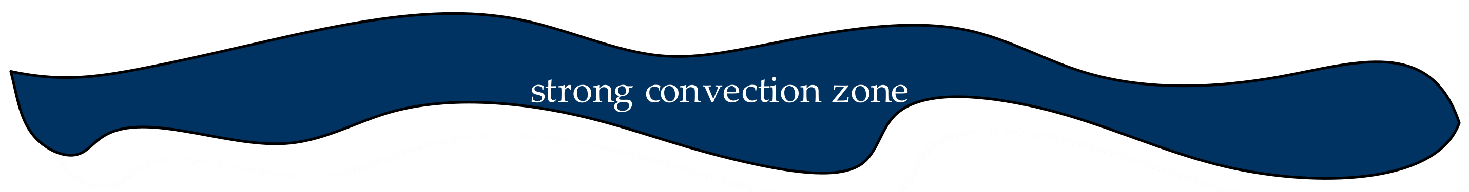
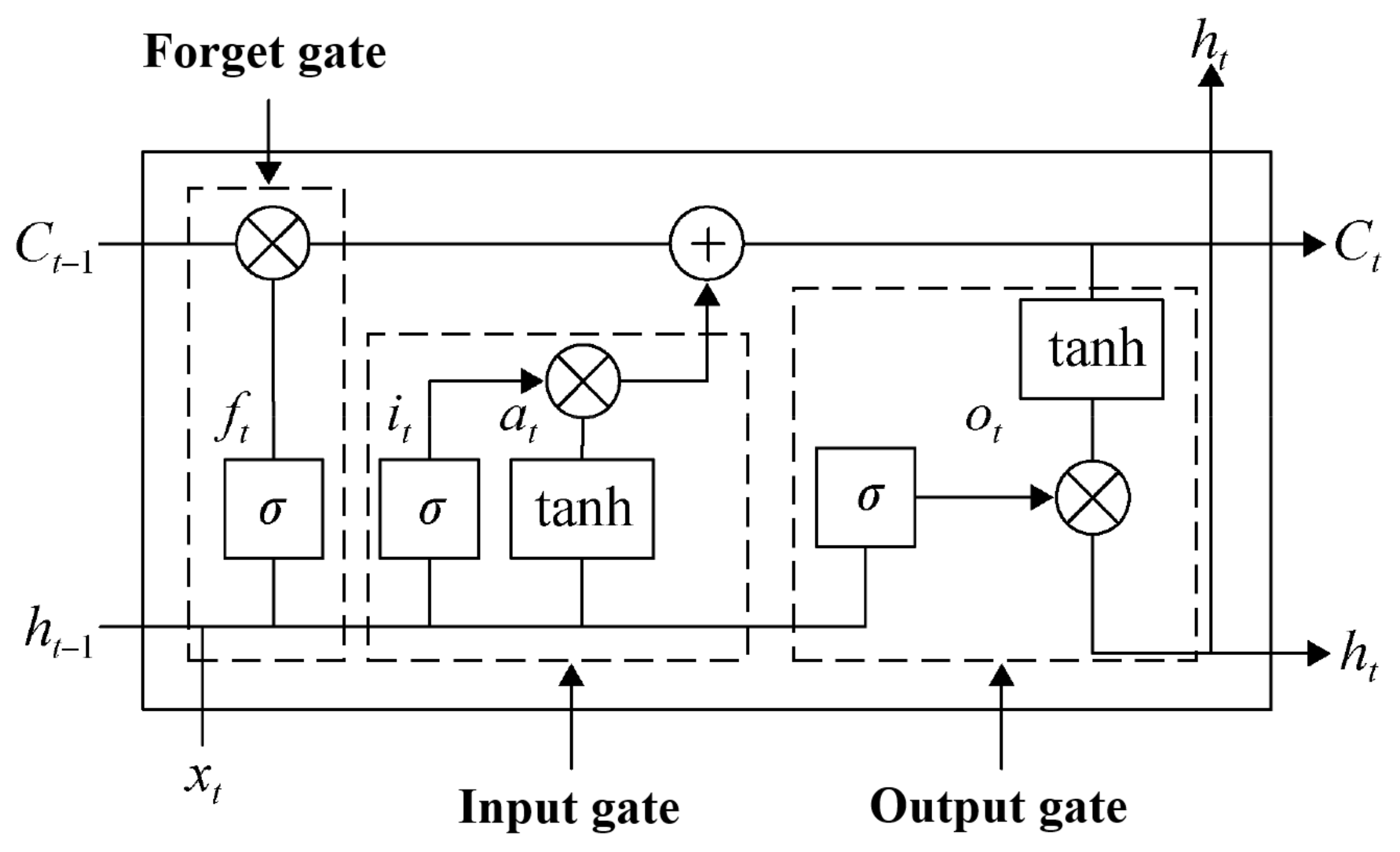
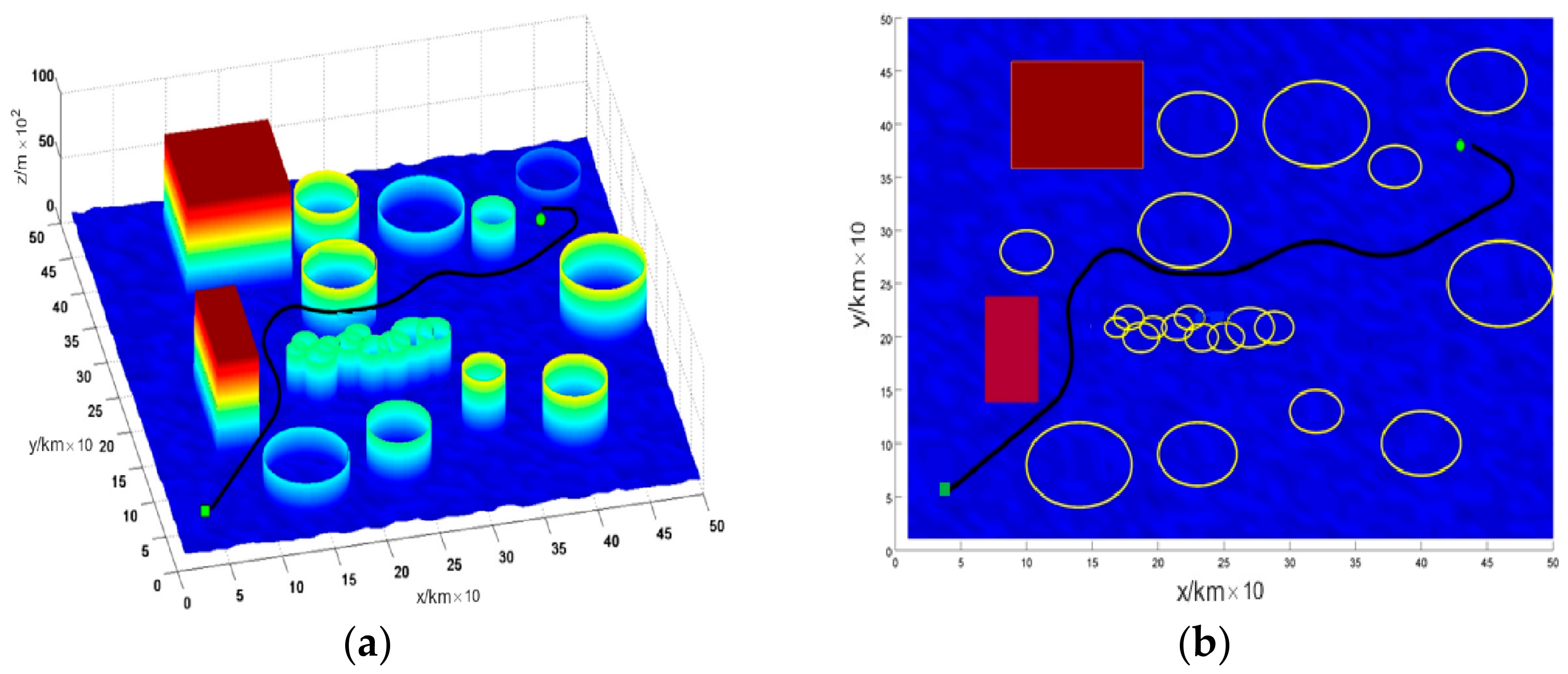
Table 1.
Topology switching table.
| Unable to Communicate | Topology | Unable to Communicate | Topology |
|---|---|---|---|
| 1, 2 | B | 2, 4 | B |
| 1, 3 | C | 2, 5 | A |
| 1, 4 | B | 3, 4 | E |
| 1, 5 | C | 3, 5 | C |
| 2, 3 | A | 4, 5 | F |
Table 2.
Experimental results under weak wind conditions without mobile threats.
| Pa/% | Pl/% | Pm/% | Ds/km | Tc/s | |
|---|---|---|---|---|---|
| Algorithm in this paper | 100 | 0 | 0 | 876.71 | 62.95 |
| Algorithm in [12] | 100 | 0 | 0 | 737.03 | 23.90 |
| Algorithm in [37] | 99 | 1 | 0 | 826.22 | 49.46 |
| Algorithm in [46] | 100 | 0 | 0 | 869.97 | 60.25 |
Table 3.
Experimental results under strong wind conditions without mobile threats.
| Pa/% | Pl/% | Pm/% | Ds/km | Tc/s | |
|---|---|---|---|---|---|
| Algorithm in this paper | 100 | 0 | 0 | 905.16 | 63.42 |
| Algorithm in [12] | 92.5 | 2 | 5.5 | 786.49 | 29.08 |
| Algorithm in [37] | 69.5 | 7 | 23.5 | 953.57 | 50.22 |
| Algorithm in [46] | 98 | 0 | 2 | 893.64 | 66.13 |
Table 4.
Experimental results under wind conditions with mobile threats.
| Pa/% | Pl/% | Pm/% | Ds/km | Tc/s | |
|---|---|---|---|---|---|
| Algorithm in this paper | 99 | 0 | 1 | 936.72 | 67.34 |
| Algorithm in [12] | 92 | 4.5 | 3.5 | 897.59 | 32.20 |
| Algorithm in [37] | 67.5 | 6 | 26.5 | 1037.28 | 52.23 |
| Algorithm in [46] | 96.5 | 2 | 1.5 | 952.82 | 70.47 |
Table 5.
RMSE comparison table.
| Algorithm | Method in This Paper | PSO-LSTM | GA-LSTM | LSTM |
|---|---|---|---|---|
| RMSE/10−3 | 0.5031 | 0.9057 | 1.1069 | 1.7361 |
Disclaimer/Publisher’s Note: The statements, opinions and data contained in all publications are solely those of the individual author(s) and contributor(s) and not of MDPI and/or the editor(s). MDPI and/or the editor(s) disclaim responsibility for any injury to people or property resulting from any ideas, methods, instructions or products referred to in the content. |
© 2024 by the authors. Licensee MDPI, Basel, Switzerland. This article is an open access article distributed under the terms and conditions of the Creative Commons Attribution (CC BY) license (https://creativecommons.org/licenses/by/4.0/).
Share and Cite
MDPI and ACS Style
Fan, X.; Li, H.; Chen, Y.; Dong, D. A Path-Planning Method for UAV Swarm under Multiple Environmental Threats. Drones 2024, 8, 171. https://doi.org/10.3390/drones8050171
AMA Style
Fan X, Li H, Chen Y, Dong D. A Path-Planning Method for UAV Swarm under Multiple Environmental Threats. Drones. 2024; 8(5):171. https://doi.org/10.3390/drones8050171
Chicago/Turabian StyleFan, Xiangyu, Hao Li, You Chen, and Danna Dong. 2024. "A Path-Planning Method for UAV Swarm under Multiple Environmental Threats" Drones 8, no. 5: 171. https://doi.org/10.3390/drones8050171