

Constrained State Regulation Problem of Descriptor Fractional-Order Linear Continuous-Time Systems

1
College of Mathematics and Systems Science, Shandong University of Science and Technology, Qingdao 266590, China
2
Faculty of Economics and Business Administration, St. Kl. Ohridski Sofia University, 1113 Sofia, Bulgaria
*
Authors to whom correspondence should be addressed.
Fractal Fract. 2024, 8(5), 255; https://doi.org/10.3390/fractalfract8050255
Submission received: 28 February 2024
/
Revised: 9 April 2024
/
Accepted: 23 April 2024
/
Published: 25 April 2024
(This article belongs to the Special Issue Numerical Solutions of Caputo-Type Fractional Differential Equations and Derivatives)
Abstract
:This paper deals with the constrained state regulation problem (CSRP) of descriptor fractional-order linear continuous-time systems (DFOLCS) with order . The objective is to establish the existence of conditions for a linear feedback control law within state constraints and to propose a method for solving the CSRP of DFOLCS. First, based on the decomposition and separation method and coordinate transformation, the DFOLCS can be transformed into an equivalent fractional-order reduced system; hence, the CSRP of the DFOLCS is equivalent to the CSRP of the reduced system. By means of positive invariant sets theory, Lyapunov stability theory, and some mathematical techniques, necessary and sufficient conditions for the polyhedral positive invariant set of the equivalent reduced system are presented. Models and corresponding algorithms for solving the CSRP of a linear feedback controller are also presented by the obtained conditions. Under the condition that the resulting closed system is positive, the given model of the CSRP in this paper for the DFOLCS is formulated as nonlinear programming with a linear objective function and quadratic mixed constraints. Two numerical examples illustrate the proposed method.
1. Introduction
Descriptor systems can be considered a powerful modeling tool since they can describe processes governed by differential and algebraic equations [1]. They play an important role in the field of system control theory because of their extensive practical background, such as in chemistry, robotics, and circuit systems [2,3,4]. CSRP is a basic problem in control systems in that there are always hard constraints on states and control inputs in practical engineering problems. When addressing constraints problems, an effective and generic approach relies on the invariance of polyhedral sets, an aspect thoroughly explored in [5,6,7,8,9]. In [10,11], the CSRP of descriptor integer order linear continuous-time systems has been discussed by reformulating the descriptor systems into equivalent state-space systems, and solutions are obtained by using the invariant sets methods.
Compared to integer-order differential equations, fractional-order differential equations can more accurately describe system behavior, especially in systems with memory effects and long-range dependencies. Due to the memory effects of fractional-order derivatives, they can better reflect the influence of the system’s historical states on its current state. Therefore, the theory and methods of fractional-order systems have wide applications in various fields such as control theory, signal processing, biomedical engineering, economics, physics, and more [12,13]. Researchers have conducted extensive studies on fractional-order systems, including stability [14], synchronization [15], and state estimation [16]. Moreover, in [17,18,19,20], the basic problems of stability and reachability of fractional-order positive systems are studied. Descriptor systems provide a more precise description of system non-linearity and complexity, thus offering better adaptability and performance in handling complex real-world problems. These advantages give descriptor systems an important position and promising prospects in scientific research and engineering applications. Hence, there are also many research results on descriptor fractional-order systems. The basic theory and application of the descriptor fractional-order system are studied in [21,22,23]. However, there are few studies on the CSRP of descriptor fractional-order systems. For example, in [24], a class of decentralized controllers for descriptor fractional-order positive systems stabilization is designed, and the solution of the controller gain matrix is given. However, state and control constraints were not considered in the above research. In practical engineering problems with state constraints, the stability of the system is a premise condition of the normal operation of the control system [25,26]. Because of the particularity of fractional calculus, methods of the integer order system cannot be directly applied to the fractional-order system with state constraints, which makes it necessary to study the constrained state regulation of DFOLCS.
Based on above reasons, the purpose of this work is to design the linear state feedback controller for the DFOLCS. We address the CSRP of DFOLCS by virtue of positively invariant set (PIS) theory in this paper. The necessary and sufficient conditions for the existence of a polyhedral PIS of the equivalent reduced system is presented, and models and corresponding algorithms for solving the CSRP of a linear feedback controller are also proposed by the obtained conditions. Under mild conditions where the resulting closed system is positive, the given model of the CSRP in this paper for the DFOLCS is formulated as nonlinear programming with a linear objective function and quadratic mixed constraints. Numerical examples illustrate the proposed method. The contributions highlighted in this paper are as follows:
(1) An equivalent fractional-order reduced system is obtained via the decomposition and separation method and coordinate transformation.
(2) A necessary and sufficient condition for the existence of polyhedral PIS in the equivalent reduced system is proposed based on PISs theory, Lyapunov stability theory, and some mathematical techniques.
(3) Two-controller design algorithm for the CSRP of generic DFOLCS is presented. Under the condition that the reduced system is positive, a nonlinear programming model is proposed, which is easily performed from a point of computational view.
The remainder of the paper is organized as following: Section 2 presents some preliminaries and formulation of the CSRP for the DFOLCS. In Section 3, an equivalent reduced system is derived by using coordinate transformation, the necessary and sufficient condition for the positive invariance of polyhedron for DFOLCS is proposed. Section 4 proposes two models and corresponding algorithms of CSRP. Section 5 concludes with illustrative examples. The paper ends with concluding remarks in Section 6.
Notations: , , and represent the n dimensional space of real vectors, the n dimensional space of positive real vectors, and the space of matrices with real entries, respectively. C is the complex number set and for any ; denotes the real part of complex number z. and represent the identity matrix and the row vector of the identity matrix , respectively. denotes the row vector of matrix A. For means all components of are nonnegative. is the rank of matrix E. is Metzler matrix with off-diagonal elements are nonnegative. means that P is positive definite (negative definite).
2. Preliminaries and Problem Formulation
2.1. Descriptor Fractional-Order Linear Continuous-Time Systems
Consider the DFOLCS
and the standard fractional-order linear continuous-time systems (SFOLCS)
where , , , is the state and control input, and , i.e., E is a rank-deficient matri, , . The SFOLCS (2) (or DFOLCS (1)) is called (internally) positive if for all initial conditions and every .
Definition 1
The initial information about lacks adequacy for forecasting the system’s future behavior. Consequently, the depiction of Equation (2) does not precisely qualify as a state-space representation and is termed a “pseudo state-space”. Assuming for the solution to system (2) is expressed as:
If system (2) with constant history, in other words, for , the initialization function is given by
thus, one has
where is the Mittag-Leffler function, which is defined as follows: .
Definition 2.
Set P is the PIS of the dynamical system (1) (or (2)) if and only if where is the trajectory of
2.2. Problem Formulation
For DFOLCS (1), the state constraints polyhedral set is defined by
where with and
The CSRP of DFOLCS (1) is to be studied. The objective is to find controller such that for all initial states , the corresponding trajectory will be asymptotically stable to the origin without violating the constraints (3).
3. Positively Invariant Conditions for Equivalent Reduced Systems
Motivated by the idea of the decomposition and separation method in integer order descriptor systems, we deal with the CSRP of DFOLCS (1) in the same way.
3.1. Equivalent Reduced System
Throughout the paper, we investigate DFOLCS (1) and have the following assumption:
(A): system (1) is regular, which means that there exists at least some such that the determinant .
The regularity assumption (A) of system (1) guarantees the existence and uniqueness of the solution to system (1) [28].
Under the assumptions (A), for the DFOLCS (1), there must exist two nonsingular matrices and ( and can be obtained by preforming the elementary row and column transformations on the identity matrix ) such that
where
, ,
,
Define the new state vector
We have
Since the DFOLCS (1) is not necessarily impulse-free, is not necessarily invertible. The impulse elimination algorithm based on dynamic decomposition is presented below.
Step 1: Perform decomposition procedure (4) for the DFOLCS (1).
Step 2: Find a matrix satisfying , suppose . Under the assumption of impulse controllability, , such a is solvable.
Step 3: Find a makes
Remark 1.
The impulsive behavior that appears in the response of the DFOLCS is due to the singularity of matrix . If the descriptor system is completely controllable (at its finite and infinite modes), the matrix has a full row rank, and there exists a state feedback law such that the closed loop system does not exhibit impulsive modes and has pre-specified finite modes [10].
By the impulse elimination algorithm based on dynamic decomposition and Remark 1, system (1) is completely controllable if there exists a feedback control
where such that the matrix is invertible and is the feedback control law for the reduced system. The aim of this step is to separate the feedback control law of the reduced system. By substituting in system (1) with (5), we have:
from (4), there always exists two nonsingular matrices and such that
Let coordinate transformation
thus,
From Remark 1 and assumptions A, system (6) is regular and does not exhibit impulsive modes if there exist two nonsingular matrices and ( and can be obtained by performing the elementary row and column transformations on the identity matrix ), such that [28]:
substituting (9) with (10), the system (6) is transformed into
the DFOLCS (1) is transformed into
By choosing the state feedback law with , system (12) is an equivalent reduced system:
Lemma 1
([18]). The equivalent reduced system (14) is positive if and only if .
Proof.
(Sufficiency) Obviously, when is a Metzler matrix, and the solution of Equation (14), i.e., for . Thus, we obtain that system (14) is a positive matrix. □
(Necessity) For (the i-th column of the identity matrix ), the trajectory of the system does not leave the orthant only if , which implies for . The matrix has to be a Metzler matrix.
From (8), (3) can be rewritten as:
from (13), , by choosing the state feedback control with we have
and , the polyhedral set (3) becomes the following form:
Hence, a consequence of the above result is the following Proposition:
Proposition 1.
The polyhedral set is PIS of DFOLCS (1) if and only if the polyhedral set is PIS of the reduced system (14).
Proof.
Assume that is PIS of DFOLCS (1); we have ; the polyhedral set is PIS of the reduced system (14), and we have . □
By lemma 1 in [10], if and only if .
Next, we provide the necessary and sufficient condition for the fractional-order polyhedral set to be a PIS.
3.2. Positive Invariance of Fractional Order Polyhedral Sets
Let a condition that the polyhedron is PISs of the equivalent reduced system (14) will be discussed in the sequel.
Proposition 2
([29,30]). (P1): Hypothetical existence of Lyapunov function and class-κ functions satisfy:
where then system (14) is asymptotically stable.
(P2): system (14) is asymptotically stable if and only if
where is the eigenvalue of matrix .
(P3): system (14) is asymptotically stable if there exist a matrix , , such that
Theorem 1.
The polyhedral set,
with is a PIS of system (14) if and only if
is not increasing along the trajectory of system (14).
Proof.
If , , then because is a positively invariant. By Proposition 2, the is negative definite; hence,
Hence,
is not increasing along the trajectory of system (14). □
By , one has
the initial condition satisfies then and since is not increasing along the trajectory of system (14). In the sequel,
so the polyhedral set is a PIS of system (14).
It is known that for integer order systems, if and such that then the equilibrium of system (14) is stable in the sense of Lyapunov [29]. In the following proposition, we will show that these conditions also imply the positive invariance of the set for the positive fractional-order system.
When the matrix degenerates into the identity matrix , we have the following proposition:
Proposition 3
To obtain the algebraic conditions for the polyhedral set to be a PIS, the following propositions are proposed:
Proposition 4
From Proposition 4, Proposition 5 can be obtained.
Proposition 5.
The polyhedral set is a PIS of system (14), then,
Proof.
is a PIS of system (14), by Theorem 1, is not increasing along the trajectory of system (14). □
If , then then
by Proposition 4, one has
Since
then substitute (20) with (21), Then , because and
For the initial state implies By the arbitrariness of ,
The following result will also be used in the sequel.
Proposition 6
([5]). If and implies for then there exists a matrix such that
Proof.
The row rectors and of the matrices and belong to the same r-dimensional subspace of that is orthogonal to the -dimensional null space of the matrix , according to lemma 2 in [5]; by , we obtain there exists a matrix such that □
An algebraic condition for a polyhedral set to be a positive invariant for system (14) is presented in Theorem 2.
Theorem 2.
The polyhedral set,
with is a PIS of system (14) if and only if there exists a matrix such that
and
Proof. Necessity.
is a positively invariant, by Proposition 5, it yields
from Proposition 6, one has
Thus, one can obtain
and
If then, from (24), it yields Hence,
since
Therefore, the polyhedral set is a PIS of system From Proposition 3,
Sufficiency. Because according to (22), if then,
Thus, and By Proposition 3, one can obtain
one has
Hence, the polyhedral set is a PIS of system (14).
Next, the polyhedral set is proven to be a PIS for system (14) in Theorem 3. □
Theorem 3.
The polyhedral set
with , is a PIS of system (14) if and only if there exists a matrix H such that
and
with , and
Proof.
By (27), we have
Substitute (25) with (28); it yields
by (26), one has
Let , , and by (29) and (30), one can obtain
by Theorem 2, the polyhedral set is a PIS of system (14); thus, is a PIS of system (14). From (28) and (29), if and only if ; therefore, is a PIS of system (14) if and only if there exists a matrix such that and □
If the reduced system (14) is a standard fractional-order positive linear continuous-time system, the following lemma gives the asymptotical stability conditions of the system (14).
Lemma 2
([18]). The system (14) remaining positive is asymptotically stable if there exists a vector such that
4. The Controller Design Algorithm
It is obvious that the control law is a solution to the CSRP if and only if system (1) is completely controllable (that is does not exhibit impulsive modes) and for all initial states , which satisfies inequalities (3), the corresponding trajectory asymptotically stable to the origin and without violating the constraints (3).
This condition can also be expressed by the following Theorem 4.
Theorem 4.
The control law is a solution to the CSRP for system (1) if and only if the following conditions are satisfied:
(i) There exists an equivalent reduced system (14);
(ii) The equivalent reduced system (14) is asymptotically stable, and the polyhedral set is PIS of system (14).
Proof.
The system (1) is completely controllable (that is does not exhibit impulsive modes) if and only if there exists an equivalent reduced system (14); all initial states which satisfying inequalities (3), the corresponding trajectory is asymptotically stable to the origin and without violating the constraints (3) if and only if the equivalence reduced system (14) asymptotically stable, and the polyhedral set is PIS of system (14). Thus, satisfying conditions (i) and (ii), the control law is a solution to the CSRP for system (1). □
Case 1: If equivalent reduced system (14) is a SFOLCS. For system (1), from Theorems 3 and 4 and Proposition 2, the control law is a solution of the CSRP, which can be solved by the following methods.
Step 1: Find an equivalent reduced system (14) of system (1).
Step 2: Establish the objective function
The constraints
or
where . The first inequalities in (32) and (33) ensure the asymptotical stability of system (14); the second and third equalities ensure the polyhedron is positively invariant to system (14); is the rate of convergence. But it is difficult to find a feasible solution of (32) because of the angle constraints. For (33), it can be formulated as a linear matrix inequality (LMI) problem, which can be solved by software such as Yalmip, CVX, and so on. But if the dimension is high, it is also not easy to find the solution.
Case 2: In Case 1, if the control law make , according to Lemma 1, the equivalent reduced system (14) is a fractional order positive linear continuous-time system, from Theorems 3 and 4 and Lemma 2, the control law is a solution of the CSRP, which can be solved by the following nonlinear programming (35).
Step 1: Find an equivalent reduced system (14) of system (1).
Step 2: Establish the objective function
The constraints
where . The first inequalities in (35) ensure the system (14) is positive; the second and third inequalities in (35) ensure asymptotic stability of system (14); and the fourth and fifth inequalities ensure the polyhedron is positively invariant to system (14). is the rate of convergence and maximizes of increases the rate of convergence to equilibrium.
Remark 2.
With fixed system parameters and as well as constraint parameters and . It becomes evident from (35) that the parameter ε holds a significant correlation with the rate of convergence. Specifically, when , the largest possible value of ε guarantees the fastest convergence rate towards the equilibrium.
5. Numerical Examples
We illustrate our method with the following examples.
Example 1.
Consider the descriptor fractional order linear continuous-time system
where , E, A and B are as follows
It is easy to verify that is not identically zero, so system (36) is regular.
The constraints on the state is given by (3) with
For system (36), from Theorems 3 and 4 and Lemma 2, the feedback control is a solution to the CSRP, which can be solved by nonlinear programming.
Step 1: Find an equivalent reduced system.
By the impulse elimination algorithm based on dynamic decomposition, system (36) is impulse controllable if , according to ; we obtain ; then the impulsive behavior can be eliminated, and the corresponding gain matrix is with choose and
and can be obtained by performing the elementary row and column transformations on the identity matrix . From matrices and are given by:
then, from (10) and (11), the matrices , and can be obtained
by the controller make the equivalent reduced system can be converted to
where
Step 2: Establish the objective function
Maximize the objective function with constraints
where The third Equation in (38) is quadratic since in is unknown, which makes (38) nonlinear.
The solution of (38) gives ,
and such that
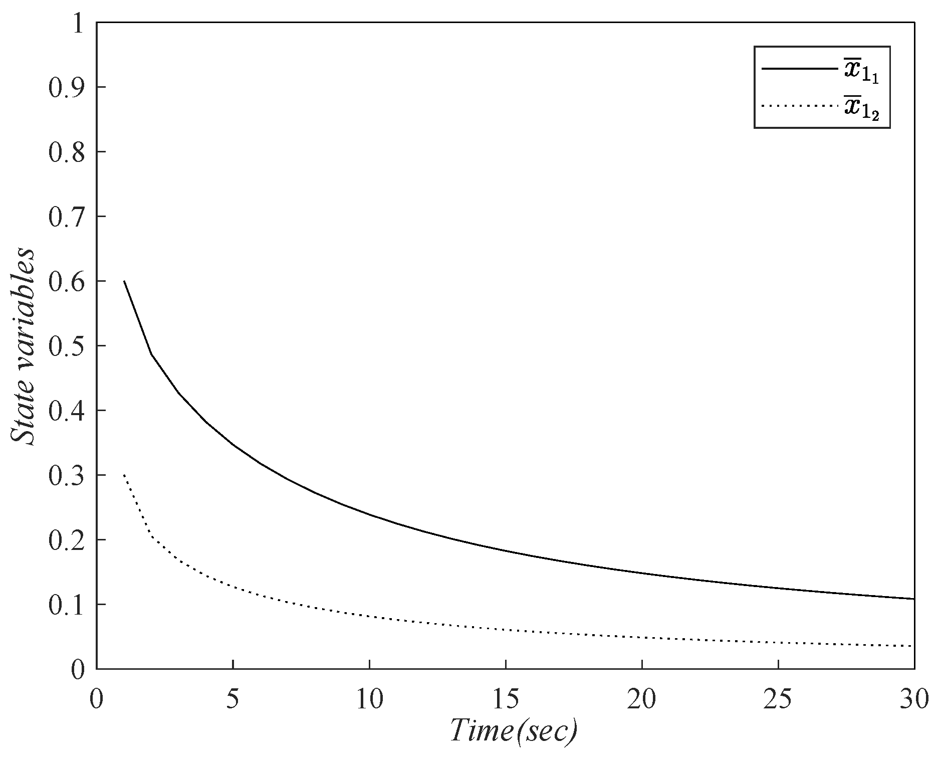
The result shows that there exists a linear state feedback controller such that all initial states that satisfy state constraints () and the corresponding trajectory of (37) is asymptotically stable and converges to the origin in the interval , which is shown in Figure 1.
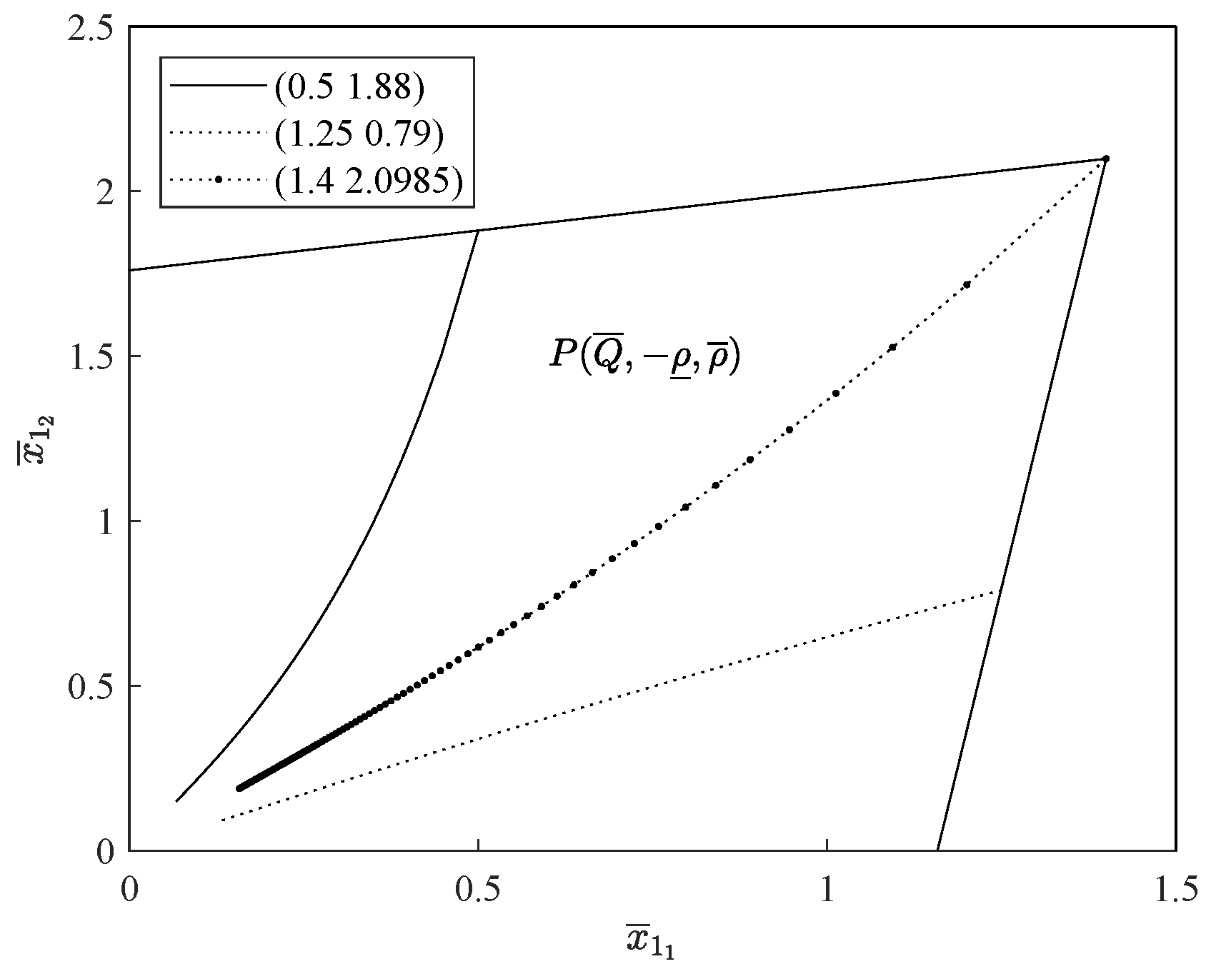
In Figure 2, the trajectories originating from the initial state are depicted, all residing within the designated constraint region.
The above results also indicate that there exists an equivalent reduced system of (37), which is asymptotically stable, and the polyhedral is PIS of system (37), from Theorem 4 and (6), the control law
where
Hence, is a solution to the CSRP of the DFOLCS (36).
Remark 3.
The reduced system (37) is not a positive system in that is not a nonnegative matrix, i.e., , but by the controller , which makes a Metzler matrix, the resulting system becomes positive system. By Lemma 1, we can guarantee the asymptotic stability and positivity of the closed loop from Lemma 2; hence, Theorem 4 is also valid.
Example 2.
We modify the state constraints in Example 1 with the state constraints in the form of (3) being given by
For system (36), by Theorem 3, Theorem 4, and Lemma2, the feedback control is a solution to the CSRP, which can be obtained by the following algorithm that can be solved by nonlinear programming.
Step 1: Find an equivalent reduced system.
By the controller , the equivalent reduced system can be transformed into
where
Step 2: Establish the objective function
Maximize the object function with constraints
where
The solution of (40) gives
and such that
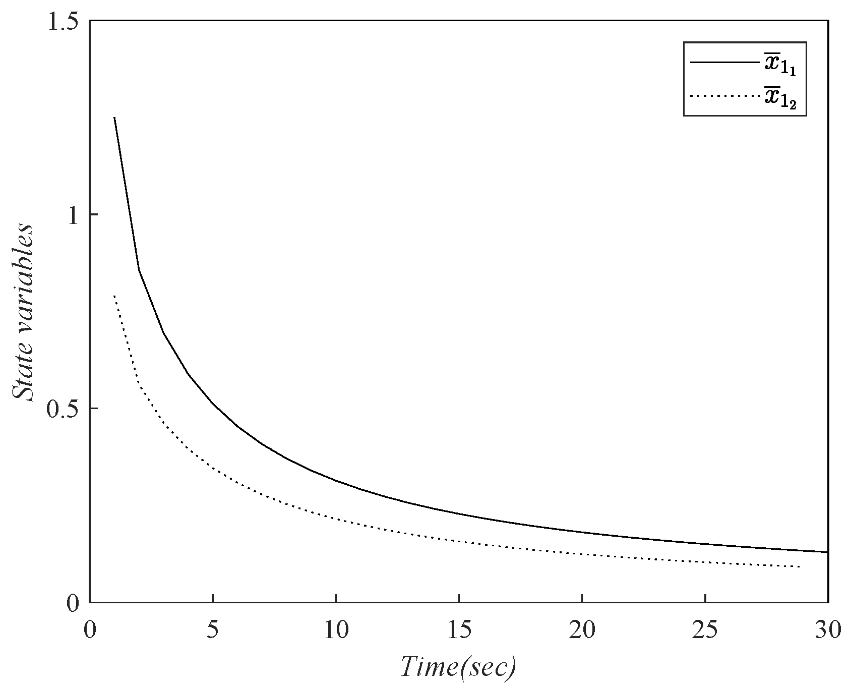
The result in Figure 3 shows that there exists a linear state feedback controller such that all initial states that satisfy state constraints are asymptotically stable and converge to the origin in the interval .
In Figure 4, trajectories emanating from the initial state are shown; they are also in the constraint region.
The above result indicates that there exists an equivalent reduced system of (39), which is asymptotically stable and converges to the equilibrium point with the polyhedral is a PIS of system (39), from Theorem 4 and (6), the control law
where
Hence, is a solution to the CSRP of DFOLCS (36).
To demonstrate the universality of the controller design scheme, we will discuss an example where E is a full-row rank matrix, meaning that the scheme remains feasible even when the DFOLCS degenerates into the SFOLCS.
Example 3.
Consider SFOLCS with
and the state constraints in the form of (3) being given by
By Theorems 3 and 4 and Lemma 2, the feedback control is a solution to the CSRP, which can be obtained by the following algorithm that can be solved by nonlinear programming (34) and (35).
The solution of (40) gives and such that
Obviously, there exists a linear state feedback controller such that all initial states that satisfy state constraints are asymptotically stable and converge to the origin. Hence, is a solution to the CSRP of SFOLCS.
Remark 4.
In practical engineering applications, state variables usually cannot be measured because of the varied and complicated work conditions, which makes state feedback impossible while dynamical output feedback can avoid the drawbacks [32,33], hence the output feedback of CSRP for DFOLCS will be an interesting topic in future research.
6. Conclusions
In this paper, the CSRP of DFOLCS is studied when . To obtain an equivalent reduced system, the decomposition and separation method and coordinate transformation are proposed. To find the necessary and sufficient conditions of positive invariance for the reduced system, the PISs theory, the Lyapunov stability theory, and some mathematical techniques are utilized. We also propose optimization models and a corresponding algorithm for finding the linear state feedback controller design of CSRP for DFOLCS. The CSRP is transformed into nonlinear programming with a linear objective function and quadratic mixed constraints. Our algorithm stands out for its ease of implementation compared to other methods. This is because the nonlinear optimization problem can be readily solved using any off-the-shelf mathematical software. Numerical examples further demonstrate the effectiveness of the proposed algorithm. An interesting question in this paper is the optimization problem (32). How to find the solution to (32) is our forthcoming research topic. The method proposed in this paper for solving CSRP is also attractive, and studying time delay and randomness helps us gain a deeper understanding of the behavior of complex systems, improve the performance and stability of systems, and optimize decision-making processes. Hence, another interesting research problem is to extend this method to delayed fractional order linear continuous-time systems and observer-based controller designs of stochastic systems [34].
Author Contributions
Conceptualization, H.Y. and X.S.; methodology, H.Y. and X.S.; software, H.Y.; validation, H.Y., X.S. and I.G.I.; investigation, H.Y.; writing—original draft preparation, H.Y.; writing—review and editing, H.Y., X.S. and I.G.I.; supervision, H.Y.; funding acquisition, H.Y. All authors have read and agreed to the published version of the manuscript.
Funding
This research received no external funding.
Data Availability Statement
No new data were created or analyzed in this study. Data sharing is not applicable to this article.
Acknowledgments
We would like to express our great appreciation to the editors and reviewers.
Conflicts of Interest
The authors declare no conflict of interest.
Abbreviations
The following abbreviations are used in this manuscript:
| CSRP | constrained state regulation problem |
| DFOLCS | descriptor fractional-order linear continuous-time systems |
| SFOLCS | standard fractional-order linear continuous-time systems |
| LMI | linear matrix inequality |
| PIS | positively invariant set |
References
- Hu, J.; Luo, R.; Dong, H.; Chen, C.; Liu, H. Dynamic event-triggered fusion filtering for multi-sensor rectangular descriptor systems with random state delay. IEEE Trans. Signal Inf. Process. Netw. 2023, 9, 836–849. [Google Scholar] [CrossRef]
- Si, X.; Yang, H.; Ivanov, I. Conditions and computation method of constrained regulation problem for a class of fractional-order nonlinear continuous-time systems. Int. J. Appl. Math. Comput. Sci. 2021, 31, 17–28. [Google Scholar]
- Terasaki, S.; Sato, K. Minimal controllability problem on linear structural descriptor systems with forbidden nodes. IEEE Trans. Autom. Control 2024, 69, 527–534. [Google Scholar] [CrossRef]
- Ge, Z. GE-semigroup method for controllability of stochastic descriptor linear systems. Sci. China Inf. Sci. 2023, 66, 139201. [Google Scholar] [CrossRef]
- Bitsoris, G. Positively invariant polyhedral sets of discrete-time linear systems. Int. J. Control 1988, 47, 1713–1726. [Google Scholar] [CrossRef]
- Ren, Y.; Er, M.J.; Sun, G. Switched systems with average dwell time: Computation of the robust positive invariant set. Automatica 2017, 85, 306–313. [Google Scholar] [CrossRef]
- Si, X.; Yang, H. Constrained regulation problem for continuous-time stochastic systems under state and control constraints. J. Vib. Control 2022, 28, 3218–3230. [Google Scholar] [CrossRef]
- Bisoffi, A.; De Persis, C.; Tesi, P. Controller design for robust invariance from noisy data. IEEE Trans. Autom. Control 2023, 68, 636–643. [Google Scholar] [CrossRef]
- Si, X.; Wang, Z.; Song, Z.; Zhang, Z. Asymptotic stabilization of delayed linear fractional-order systems subject to state and control constraints. Fractal Fract. 2022, 6, 67. [Google Scholar] [CrossRef]
- Radhy, N.; Benzaouia, A.; Boughari, H. Constrained state regulation of linear continuous-time singular systems. Syst. Anal. Modell. Simul. 2002, 42, 677–694. [Google Scholar] [CrossRef]
- Boughari, H.; Radhy, N. Regulation of linear continuous-time singular systems with constrained states and controls. Int. J. Syst. Sci. 2007, 38, 689–698. [Google Scholar] [CrossRef]
- Yang, J.; Fan, Y.; Mu, A.; Xiong, J. Dynamic analysis and suppression strategy research on a novel fractional-order ferroresonance system. Fractal Fract. 2024, 8, 24. [Google Scholar] [CrossRef]
- Tian, Y.; Xia, Q.; Chai, Y.; Chen, L.; Lopes, A.M.; Chen, Y. Guaranteed cost leaderless consensus protocol design for fractional-order uncertain multi-agent systems with state and input delays. Fractal Fract. 2021, 5, 141. [Google Scholar] [CrossRef]
- Wang, C.; Zhao, Y. Performance analysis and control of fractional-order positive systems. IET Control Theory Appl. 2019, 13, 928–934. [Google Scholar] [CrossRef]
- Liu, J.J.R.; Lam, J.; Kwok, K.-W. Necessary and sufficient conditions on consensus of general fractional-order multi-agent systems over directed networks. IEEE Trans. Netw. Sci. Eng. 2024, 11, 485–493. [Google Scholar] [CrossRef]
- Chen, L.; Chen, Y.; Lopes, A.M.; Kong, H.; Wu, R. State of charge estimation of lithium-ion batteries based on fuzzy fractional-order unscented kalman filter. Fractal Fract. 2021, 5, 91. [Google Scholar] [CrossRef]
- Mahmoud, B.; Neda, H. A numerical approach for solving a class of fractional optimal control problems via operational matrix Bernoulli polynomials. J. Vib. Control 2018, 24, 2494–2511. [Google Scholar]
- Benzaouia, A.; Hmamed, A.; Mesquine, F.; Benhayoun, M.; Tadeo, F. Stabilization of continuous-time fractional positive systems by using a Lyapunov function. IEEE Trans. Autom. Control 2014, 59, 2203–2208. [Google Scholar] [CrossRef]
- Kaczorek, T. Selected Problems of Fractional Systems Theory; Springer: Berlin/Heidelberg, Germany, 2011. [Google Scholar]
- Yang, H.; Jia, Y. New conditions and numerical checking method for the practical stability of fractional order positive discrete-time linear systems. Int. J. Nonlinear Sci. Numer. Simul. 2019, 20, 315–323. [Google Scholar] [CrossRef]
- Kaczorek, T. Positivity and stability of fractional descriptor time-varying discrete-time linear systems. Int. J. Appl. Math. Comput. Sci. 2016, 26, 5–13. [Google Scholar] [CrossRef]
- Kaczorek, T. Positivity and stability of standard and fractional descriptor continuous-time linear and nonlinear systems. Int. J. Nonlinear Sci. Numer. Simul. 2018, 19, 299–307. [Google Scholar] [CrossRef]
- Lin, C.; Chen, B.; Shi, P.; Yu, J.P. Necessary and sufficient conditions of observer-based stabilization for a class of fractional-order descriptor systems. Syst. Control Lett. 2018, 112, 31–35. [Google Scholar] [CrossRef]
- Sajewski, L. Stabilization of positive descriptor fractional discrete-time linear system with two different fractional orders by decentralized controller. Bull. Pol. Acad. Sci. Tech. Sci. 2017, 65, 827–832. [Google Scholar] [CrossRef]
- Li, D.; He, X.; Song, T.; Jin, Q. Fractional order IMC controller design for two-input-two-output fractional order system. Int. J. Control Autom. Syst. 2019, 17, 936–947. [Google Scholar] [CrossRef]
- Si, X.; Wang, Z.; Fan, Y.; Huang, X.; Shen, H. Sampled-data-based bipartite leader-follower synchronization of cooperation-competition neural networks via interval-scheduled looped-functions. IEEE Trans. Circuits Syst. I-Regul. Pap. 2023, 70, 3723–3734. [Google Scholar] [CrossRef]
- Podlubny, I. Fractional Differential Equations; Academic Press: London, UK, 1999. [Google Scholar]
- Moubarak, M.R.A.; Ahmed, H.F.; Khorshi, O. Numerical solution of the optimal control for fractional order singular systems. Differ. Equat. Dyn. Sys. 2016, 26, 279–291. [Google Scholar] [CrossRef]
- Li, Y.; Chen, Y.Q.; Podlubny, I. Stability of fractional-order nonlinear dynamic systems: Lyapunov direct method and generalized Mittag–Leffler stability. Comput. Math. Appl. 2010, 59, 1810–1821. [Google Scholar] [CrossRef]
- Li, C.P.; Zhang, F.R. A survey on the stability of fractional differential equations. Eur. Phys. J.-Spec. Top. 2011, 193, 27–47. [Google Scholar] [CrossRef]
- Mozyrska, D.; Torres, D. Modified optimal energy and initial memory of fractional continuous-time linear systems. Signal Process. 2011, 91, 379–385. [Google Scholar] [CrossRef]
- Eshaghi, S.; Kharrati, H.; Badamchizadeh, M.A.; Hasanzadeh, I. A predictive controller based on dynamic matrix control for a non-minimum phase robot manipulator. Int. J. Control Autom. Syst. 2012, 10, 574–581. [Google Scholar] [CrossRef]
- Wang, X.; Tan, C.P. Dynamic output feedback fault tolerant control for unmanned underwater vehicles. IEEE Trans. Veh. Technol. 2020, 69, 3693–3702. [Google Scholar] [CrossRef]
- Zhen, L.A.; Hrk, B.; Jy, A. Passivity-based robust sliding mode synthesis for uncertain delayed stochastic systems via state observer. Automatica 2020, 111, 108596. [Google Scholar]
Figure 1.
The state trajectory of the system (37).

Figure 2.
The trajectory emanating from the initial state.

Figure 3.
The state trajectory of the system (39).

Figure 4.
The trajectory emanating from the initial state.

Disclaimer/Publisher’s Note: The statements, opinions and data contained in all publications are solely those of the individual author(s) and contributor(s) and not of MDPI and/or the editor(s). MDPI and/or the editor(s) disclaim responsibility for any injury to people or property resulting from any ideas, methods, instructions or products referred to in the content. |
© 2024 by the authors. Licensee MDPI, Basel, Switzerland. This article is an open access article distributed under the terms and conditions of the Creative Commons Attribution (CC BY) license (https://creativecommons.org/licenses/by/4.0/).
Share and Cite
MDPI and ACS Style
Yang, H.; Si, X.; Ivanov, I.G. Constrained State Regulation Problem of Descriptor Fractional-Order Linear Continuous-Time Systems. Fractal Fract. 2024, 8, 255. https://doi.org/10.3390/fractalfract8050255
AMA Style
Yang H, Si X, Ivanov IG. Constrained State Regulation Problem of Descriptor Fractional-Order Linear Continuous-Time Systems. Fractal and Fractional. 2024; 8(5):255. https://doi.org/10.3390/fractalfract8050255
Chicago/Turabian StyleYang, Hongli, Xindong Si, and Ivan G. Ivanov. 2024. "Constrained State Regulation Problem of Descriptor Fractional-Order Linear Continuous-Time Systems" Fractal and Fractional 8, no. 5: 255. https://doi.org/10.3390/fractalfract8050255