
Time-Specific Thresholds for Batch Process Monitoring: A Study Based on Two-Dimensional Conditional Variational Auto-Encoder


1
State Key Laboratory of Food Science and Technology, Jiangnan University, Wuxi 214122, China
2
Key Laboratory of Advanced Process Control for Light Industry (Ministry of Education), Jiangnan University, Wuxi 214122, China
3
Department of Chemical and Biological Engineering, Hong Kong University of Science and Technology, Hong Kong
*
Author to whom correspondence should be addressed.
Processes 2024, 12(4), 682; https://doi.org/10.3390/pr12040682
Submission received: 8 February 2024
/
Revised: 7 March 2024
/
Accepted: 26 March 2024
/
Published: 28 March 2024
(This article belongs to the Special Issue Data-Based Process Monitoring, Process Control, and Quality Improvement in Industry)
Abstract
:This paper studies the use of varying threshold in the statistical process control (SPC) of batch processes. The motivation is driven by how when multiple phases are implicated in each repetition, the distributions of the features behind vary with phases or even the time; thus, it is inconsistent to uniformly bound them by an invariant threshold. In this paper, we paved a new path for learning and monitoring batch processes based on an efficient framework integrating a model termed conditional dynamic variational auto-encoder (CDVAE). Phase indicators are first used to split the data and are then separated, serving as an extra input for the model in order to alleviate the learning complexity. Dissimilar to the routine using features across all timescales, only features relevant to local timestamps are aggregated for threshold calculation, producing a varying threshold that is more specific for the process variations occurring among the timeline. Leveraged upon this idea, a fault detection panel is devised, and a deep reconstruction-based contribution diagram is illustrated for locating the faulty variables. Finally, the comparative results from two case studies highlight the superiority in both detection accuracy and diagnostic performance.
1. Introduction
In the modern industrial landscape, batch processing is now widely performed in producing many high-value-added products, ranging from daily necessities to bio-pharmaceuticals to the most advanced silicones [1,2,3]. A typical batch process is composed of an ordered set of physio-chemical treatments, converting feedstock into a product with an intended specification [4]. During repetitions, these treatments not only entail a high precision in each single phase, a time window where a specific treatment is applied, but also mandate stability from one batch to another to secure the consistency among repeated products. However, such a pursuit can be substantially threatened by the occurrence of uncertainties that cannot be foreseen and assuaged by in situ controllers. Therefore, to detect abnormal deviations, process monitoring has now emerged as an integral part of batch process control systems.
So far, there are two sought-after directions drawing efforts from the process monitoring community. One is mainly prompted by sophisticated process knowledge, implicating parameter identification and subsequent residual generation for anomaly analysis and detection. The other branch is dominated by data, where the proliferation of statistical theory and machine learning has significantly boosted progression in the past three decades. Both pros and cons exist in these two directions. However, currently, data are extensively available, and the knowledge is no longer as convenient to acquire as before [5,6,7]. Consequently, the data-driven-based process monitoring, also known as SPC, has gained increasing favor for facilitating the efficient control of normal multivariate process operations [8,9,10,11,12,13].
The central task of SPC is to ascertain whether the ongoing process is normal or not according to the working statistics drawn from the query samples. Specifically, the statistic is compared with a value, also referred to as the threshold, to signal a faulty sample if it is falling beyond and a normal sample if otherwise. The SPC performance, including both the rates of Type I and II errors, is directly influenced by the threshold determination. However, the selection of the threshold heavily depends on the distribution underlying the statistics. Thus, a statistic distribution that is invariant across different time and normal conditions while being sensitive to the investigated abnormality is of paramount significance for the success of a SPC routine.
To date, many state-of-the-art methods have been devised to formulate a statistic that outperforms with respect to the aspects prescribed above. For instance, the PCA-based control charts and associated modifications are all committed to transforming the raw data into a reduced set of independent features, thus employing Hoteling’s statistic, under the presumed gaussianity. After that, other machine learning methods, such as CCA and PLS [14,15,16] as well as some deep unsupervised architectures [17,18,19,20,21], also value this idea and are devoted to the construction of the same statistic from the reduced space of transformed features. It was until the inception of the variational auto-encoder (VAE) that deep learners switched focus on using strong transformation to secure the distribution premise before using them for threshold determination [22,23,24,25,26,27]. Methods akin to these ideas can be easily found in the applications for both continuous and batch processes. However, some unique characteristics have also been reported in terms of their negative impacts on stabilizing the testing statistic, e.g., a series of studies can be cited in addressing the coupled nonlinearity and dynamicity that impede the statistical application [28,29,30,31]. As for issues linked to batch processes, its significant kinetics along the time and batch directions, known as 2D dynamics, has been the major slot for SPC professionals to fit their work into [14,32,33]. To this extent, works relevant to variable selection, process, and phase divisions have been intensively investigated to conclude a compact feature space for monitoring [28,34]. However, with the many efforts made in enhancing the model for a stable and fault-sensitive distribution, it is never an easy task to squeeze a process with varying conditions into a unified-shaped feature manifold for monitoring.
On the other hand, the multiple phases inherent to batch processes also add to the difficulties against feature extraction. To mitigate it, some composite frameworks have been proposed to cluster or classify the data to each phase beforehand, and then a secondary round of modeling is applied to each group of data to estimate the distribution [35,36]. However, these routes usually involve a hierarchy of complex procedures without a convenient framework for general batch processes. In addition, the number of clusters for phase division lacks criteria for determination, and it may also risk obfuscating some nuanced variations within each phase or even at specific timestamps.
In a nutshell, the application of SPC mandates a stable feature distribution from the time sequence, while in batch processes, being substantially challenged by unsteady states and their heterogeneity is prompted by the multiple phases. This awkward situation persists and tends to elevate the model towards the unexpendable level of complexity, rendering the risk of overfitting; however, it has so far not been assuaged in the community. Thus, it necessitates a monitoring scheme that is light in multiple-phase batch process modeling and has a tenable path for generating the threshold for intra- and inter-batch uncertainties detection. Motivated by this, research on time-specific thresholds is dissected in this paper for batch process monitoring. In light of the end-to-end advantage shown by the VAE approach, a conditional learning mechanism is first designed and interfaced with the input and latent layer of the backbone of conventional VAE to alleviate the burden of accommodating features from the multiple phases. Prior to the model, a sliding window spanning across both the time and batch directions, termed a 2D regular feature aggregator, is used to collect the samples for the model to learn from the relevant history. Once the model is trained and fine-tuned, assuming that the skeleton of process data is well boiled down to the features inside the model, only features tied to the current timeframe are lumped for the estimation and threshold determination, making a time-specific varying threshold for the 2D monitoring of batch processes. Together, the proposed framework can align with the real-world notion that batch-wise variation is easier for finding a stable pattern than only along the flattened time direction, which enables the process knowledge to be efficiently integrated into the data-driven-based method design.
The remainder of this paper is organized as follows. Section 2 performs a brief theoretical review of the variational auto-encoder. The derivation of the CDVAE, with detailed steps of process monitoring, is elaborated in Section 3. Section 4 verifies the merits of the proposed CDVAE through a penicillin fermentation and a practical fed-batch fermentation process of L. plantarum. Finally, the conclusion is summarized in Section 5.
2. Preliminaries
VAE is proposed for dealing with the probability inference problem of the generative probability model , where is a sample of and denotes the latent variables of the generative model [37]. The VAE model can be derived by approximating the intractable distribution with the variational distribution . A derivation can be derived by maximizing the likelihood :
Furthermore, satisfies the following equation according to Jensen’s inequality:
where the second term of Equation (2) is equal to , which is used to measure the discrepancy of and . The is the Kullback–Leibler (KL) divergence [26]. This term reasonably serves as the evidence of the lower bound when maximizing , which is:
Generally, is assumed to conform to the standard normal distribution . The “reparameterization trick” is applied to VAE networks to implement loss backpropagation.
3. Methodology
3.1. Batch Data Description
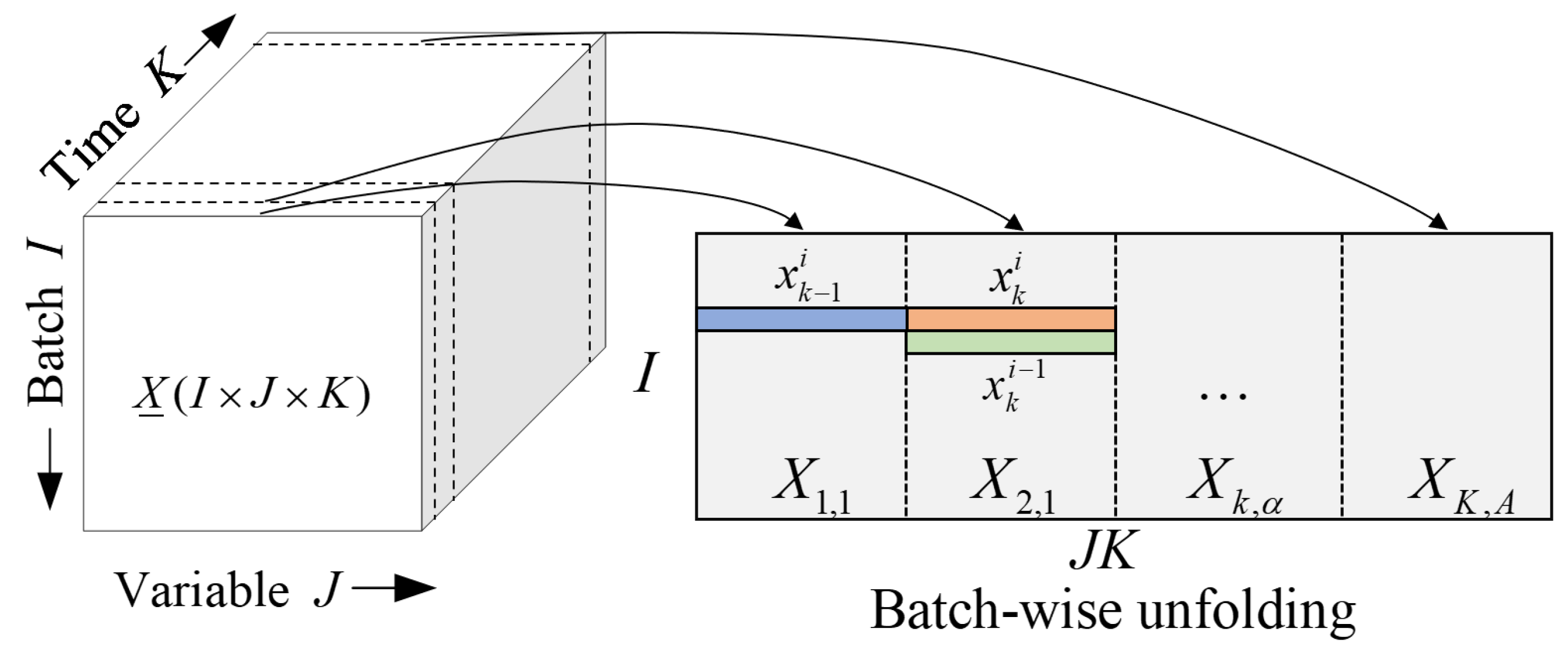
The batch process history data are stored as a three-dimensional matrix , where , , and represent the batches, variables, and samples number. Before modeling, we first unfold the three-dimensional batch process data into the two-dimensional matrix . is the th time slice in the th phase, where is defined as the number of phases according to historical experience. Then, the two-dimensional matrix is standardized by the “Z-score”.
Two-dimensional dynamic characteristics refer to the correlation of batch process data in the time-wise and batch-wise directions. Extracting two-dimensional features from batch process data can improve the model’s fault detection capabilities. For this purpose, a two-dimensional sliding window is designed in this paper. As illustrated in Figure 1, a sample may be affected by the previous batches and the previous sample , where , are the batch-wise and time-wise lagged length. The values of the , are crucial for improving the fault detection accuracy of the proposed model. The 2D moving window of the current sample is reorganized to . Meanwhile, the phase information is transferred to the phase label by a “One-to-Hot” function.
3.2. Structure of CDVAE Model
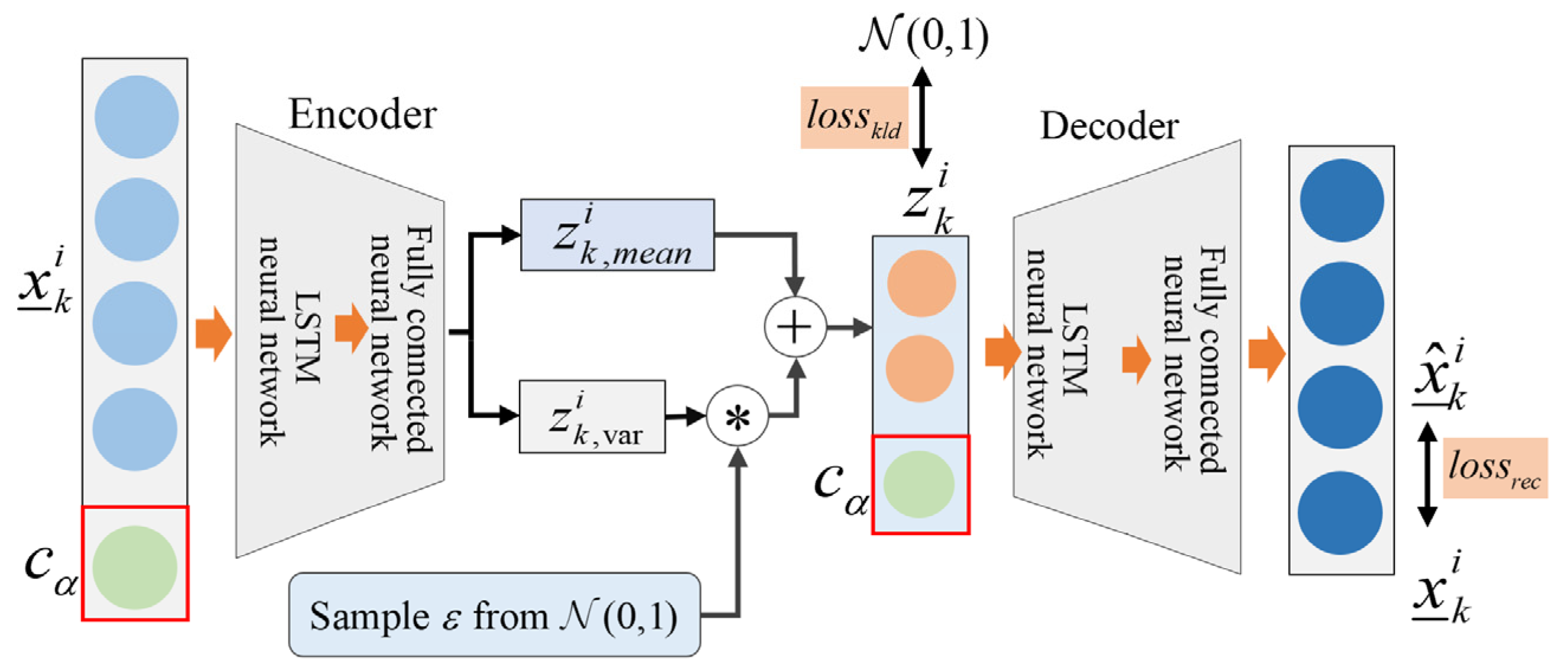
The conditional variational auto-encoder (CVAE) generates content corresponding to the input label type [38]. In the data preprocessing stage, batch process multi-phases information was transformed into the phase label . In view of this, CVAE was selected as the basic model to generate data for different periods. Meanwhile, LSTM has the ability to save previously useful information and pass it to the current input. Therefore, in order to further improve the model’s two-dimensional dynamic feature extraction capability, the LSTM network is added to the CVAE model. The combination of the LSTM network and CVAE model is named the CDVAE model. The structure of the CDVAE model is displayed in Figure 2. The input sequence and label are combined as the input data of the CDVAE model. The encoder of CDVAE includes two parts, the mean encoder and variance encoder . Then, the labels and latent variables are inputted into the decoder to generate the reconstruction . The loss function of the CDVAE model is defined as follows:
The first part of Equation (4) is the reconstruction loss in residual space, and the right part is the KL divergence loss in latent space. The reconstruction loss can be considered a mean squared error between the input sequence and reconstruction sequence, and its purpose is to penalize the reconstruction sequence as approximate to the input sequence . The KL loss term encourages the latent variable distribution to a standardized normal distribution .
3.3. Fault Detection and Diagnosis with CDVAE
3.3.1. Fault Detection
Fault detection can construct two statistics to evaluate the status of the current batch process. Two statistics are constructed from the latent and residual spaces. In the latent space, KL loss is defined as a fault detection statistic. It can be defined as follows:
where evaluates the variation of the latent variable distribution. The statistic measures the deviation between the input sequence and its reconstruction , which can be expressed as follows:
The batch process is a typical multi-period process. This paper establishes a threshold at a specific time, and the calculation steps are as follows. First, the statistics of the training data sequence are calculated based on the trained CDVAE model. Secondly, the statistics corresponding to the input sequences of different batches at the th sample are collected. Finally, kernel density estimation (KDE) is used to calculate the th threshold based on the statistics . The control limit at the th sample time is represented as follows:
where is the bandwidth and is the kernel function. The time-varying control limit calculation method at a specific moment forms a change threshold.
3.3.2. Fault Diagnosis
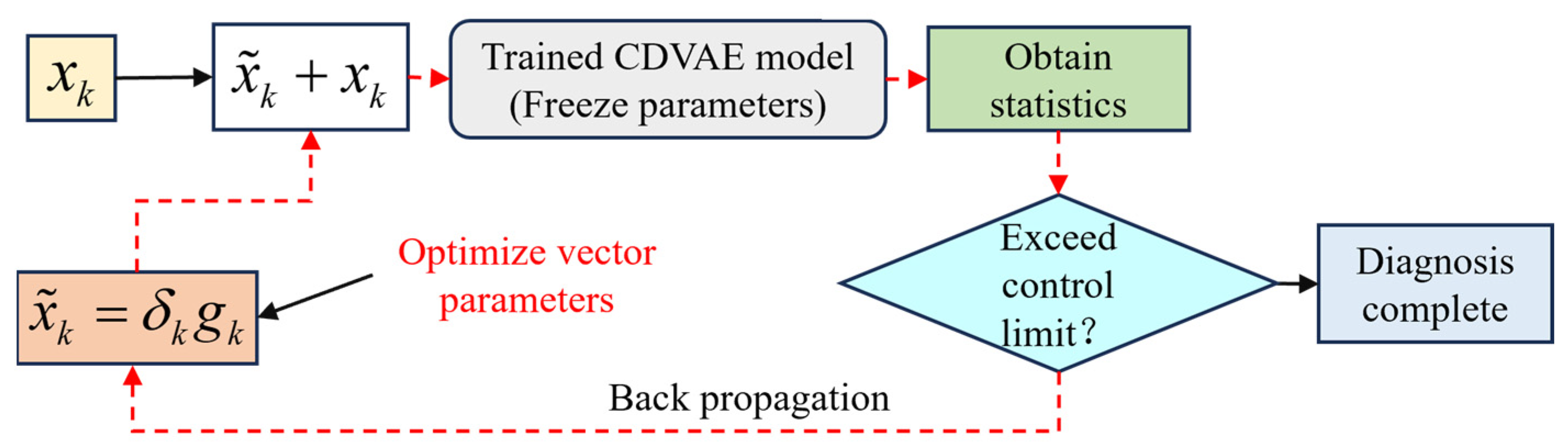
This paper proposes a novel fault diagnosis method named the DRBC diagram. This diagnosis method is inspired by the PCA-based reconstruction contribution method [39]. The DRBC structure is shown in Figure 3. Assume that the fault occurs at the th sample. The fault diagnosis method based on DRBC designs two vectors, namely the fault direction vector and the fault amplitude vector , where an element of “1” in the fault direction vector represents a variation in the corresponding variable. The amplitude vector is used to represent the degree of deviation in the current fault variable. The backpropagation mechanism is used here to optimize the product of the fault direction vector and the fault amplitude vector , which means that during the diagnosis process, the model parameters are frozen and the feedback optimization parameter is . The loss of backpropagation is the statistic data of the CDVAE. The fault diagnosis process is similar to an iterative optimization process during the model training stage. The diagnostic process repeats as indicated by the red dotted line until the statistic is below the control limit. The purpose of this is that the statistic measures the degree of agreement between the current input data and the model. Therefore, when the fault detection statistic is lower than the control limit, it means that the current data are consistent with the normal trajectory. Another advantage of DRBC is that the fault treats the trained CDVAE model as a black box and does not impose other restrictions on the model, such as differentiability. A multi-threaded diagnostic strategy can be applied to DRBC to improve the efficiency of the diagnostic process.
3.4. The Process Monitoring Framework Based on CDVAE
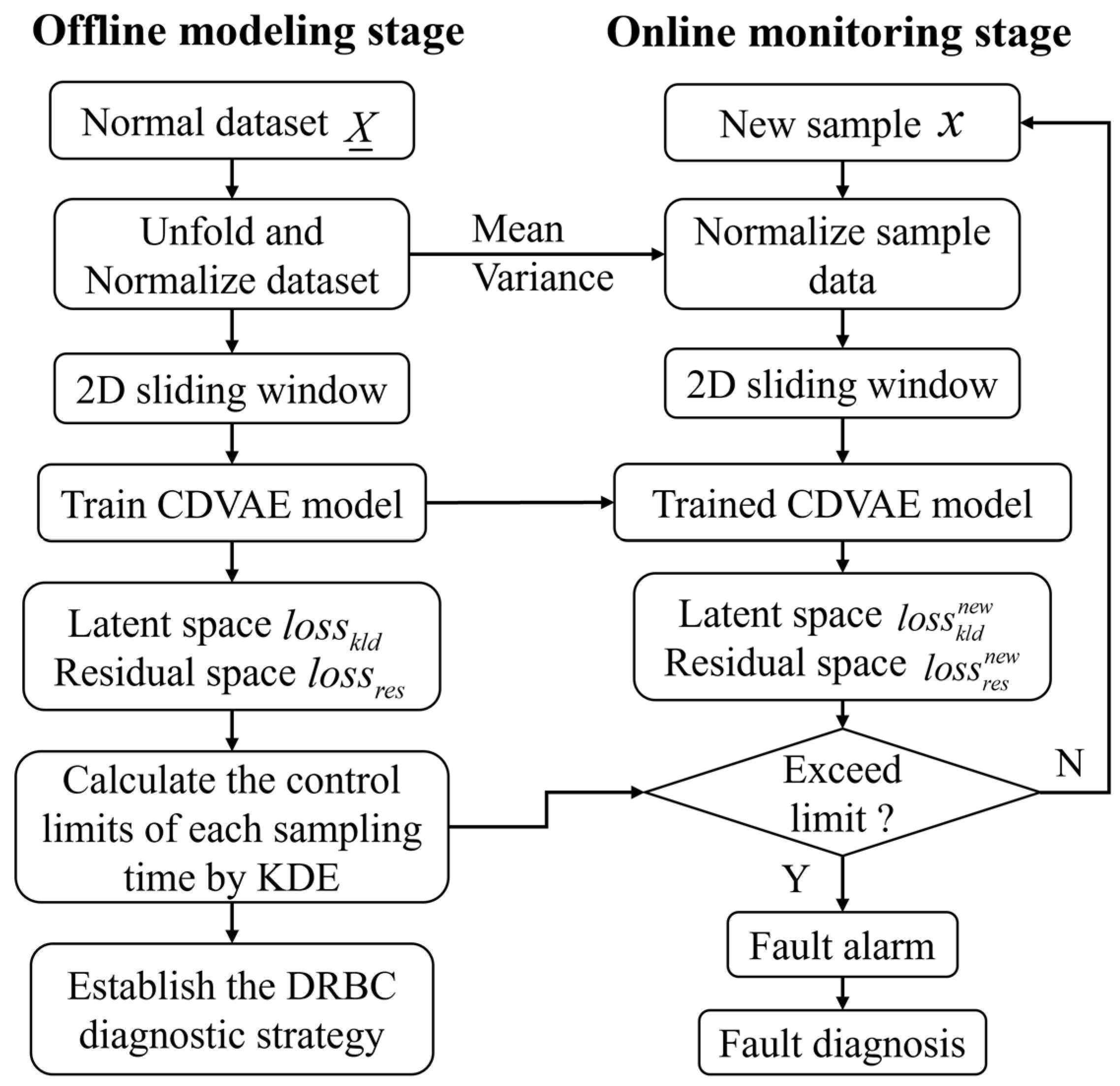
The framework of CDVAE for the batch process monitoring, consisting of the offline modeling stage and online monitoring stage, is shown in Figure 4.
Offline modeling stage:
- (a)
- Collect normal historical data;
- (b)
- Batch process data are unfolded and normalized along the batch-wise direction;
- (c)
- Establish a two-dimensional sliding window to obtain an input sequence;
- (d)
- Construct and train the CDVAE model;
- (e)
- Collect statistics corresponding to each sampling moment and use KDE to calculate the control limits of each sampling moment;
- (f)
- Establish the DRBC diagnosis approach based on CDVAE.
Online monitoring stage:
- (i)
- Collect real-time production data;
- (ii)
- Standardize sampled data using historical mean and variance;
- (iii)
- Obtain the current sampled input sequence;
- (iv)
- Use the trained CDVAE model to calculate statistics in latent and residual space;
- (v)
- Judge whether the statistics exceed the control limits;
- (vi)
- If the control limit is exceeded, DRBC is used for locating the root cause of the fault.
4. Case Study
4.1. The Penicillin Fermentation Simulation Process
4.1.1. Process Description and Modeling
In this paper, a state-of-the-art penicillin fermentation simulation platform, Pensim V 2.0 [40,41], is employed to emphasize the advantages of CDVAE.
The 120 batches are generated under normal operation conditions. A total of 100 batches are applied to train the CDVAE model, and 10 batches are used to validate the trained CDVAE model. Each batch lasts 600 h, and the interval is 0.5 h. The 2D dynamics are introduced to the batch process by assuming the substrate feed rate change in the form of Equation (8):
where and are the number of batches and sample time, denotes the random noise, and defines the dynamic factor. We define in normal batches. The 11 variables are displayed in Table 1. Changes in bacterial concentration were used as the basis for dividing periods. In this study, the batch process data are divided into three periods in the time dimension: phase 1: 0–150; phase 2: 150–1100; and phase 3: 1100–1200. The three phase labels are transferred as , , .
The network structure and training parameters of the CDVAE model are shown in Table 2. The first layer of the encoder of CDVAE is LSTM, the input dimension is 10, and the output dimension is 800. Then, the input dimension of the fully connected (FC) layer is 803, which is the sum of the output dimension of LSTM (800) and the dimension of the period label (3). Finally, the fully connected layer compresses the input sequence to three dimensions. In the decoder of CDVAE, the latent representation is filled with zero and decoded by LSTM. Then, the input dimension of the fully connected layer is the sum of the output dimension of LSTM (400) and the period label dimension (3). Finally, the latent features use fully connected layers to reconstruct the input sequence. In addition, the learning rate in the training model stage and DRBC-based diagnosis stage is set to 0.001. The lag lengths in the time-wise and batch-wise are set to 10 and 3, respectively. We also selected the VAE [25], CVAE [38], and LSTM-AE [28] methods for comparing the fault detection performance.
The control limits of the two statistics are calculated by the KDE function. The confidence interval was set to 99%. Fault detection rate (FDR) and false alarm rate (FAR) were selected to compare the process monitoring the performance [28].
4.1.2. Detection of the Faults
In addition, we consider 14 faults, and the specific types and fault magnitudes of different fault batches can be found in Table 3. The 14 faults consist of single-variable faults and multivariable faults. To prove that the proposed CDVAE model performs better fault detection, other popular models, such as traditional VAE, CVAE, and LSTM-AE, were selected for comparison.
The detection results of the 14 faults under different models are summarized in Table 4. The optimal monitoring results for each fault are bolded in Table 4. It can be directly seen that the FDR of the fault detection statistic of CDVAE is significantly better than that of other models. Secondly, for minor faults, such as fault 8, the FDR of CDVAE in the residual space detection index reached 89.6% and the detection index in shallow space reached 67.2, which achieved better detection results than other models. Obviously, after considering the two-dimensional dynamic characteristics of the model, the fault detection ability of the model has been significantly improved. For faults with large fault amplitudes, such as fault 3, the detection results of the four models in the residual space can reach 100%. This phenomenon shows that faults with larger fault amplitudes are easier to detect. Considering the dynamic characteristics of the batch dimension and ignoring the dynamic characteristics of the time dimension, the average detection rate of 14 faults of LSTM-AE is inferior to that of CDVAE. Furthermore, the average detection results of VAE and CVAE show that the introduction of phase information increases the ability of the deep model in shallow space as well as its sensitivity to anomalies. Finally, CDVAE has the lowest FAR in penicillin simulations.
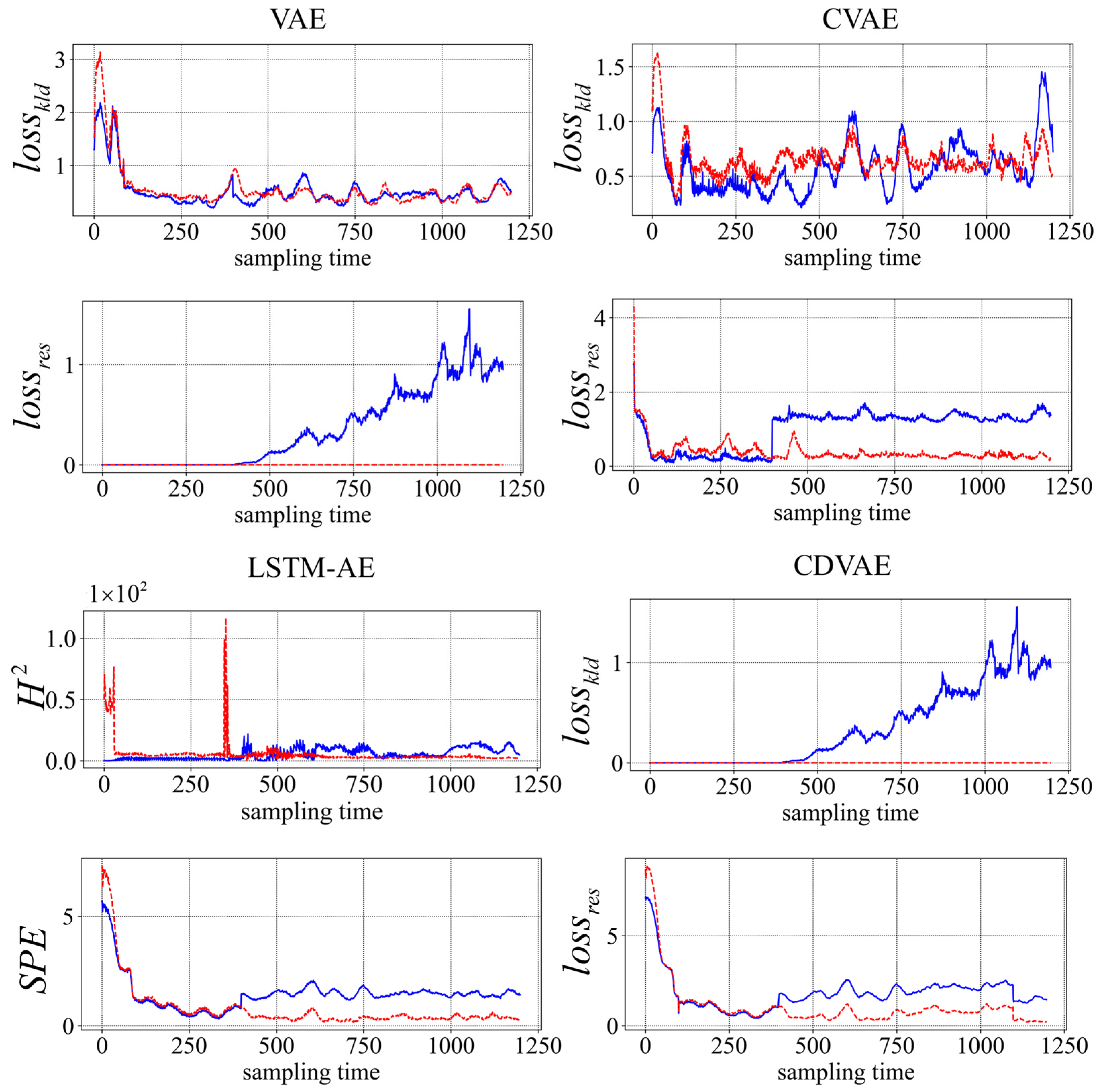
To further elaborate on the fault detection results, the fault detection plots of fault 3 under the four models are shown in Figure 5. The red dotted line is the control limit of each detection statistic, and the blue solid line is the statistics trajectory. The two detection indicators of CDVAE can quickly exceed the control limit and provide a fault alarm after the fault occurs (after the 400th sample time). LSTM-AE performs well in residual space, but its detection ability for statistics in shallow space decreases. From the fault detection diagram of the VAE and CVAE models, it can be seen that ignoring the two-dimensional dynamic characteristics greatly reduces the performance of the model in shallow space. The CDVAE model shows excellent fault detection capabilities on the penicillin simulation fermentation platform compared with other models.
4.1.3. Diagnosis of the Faults
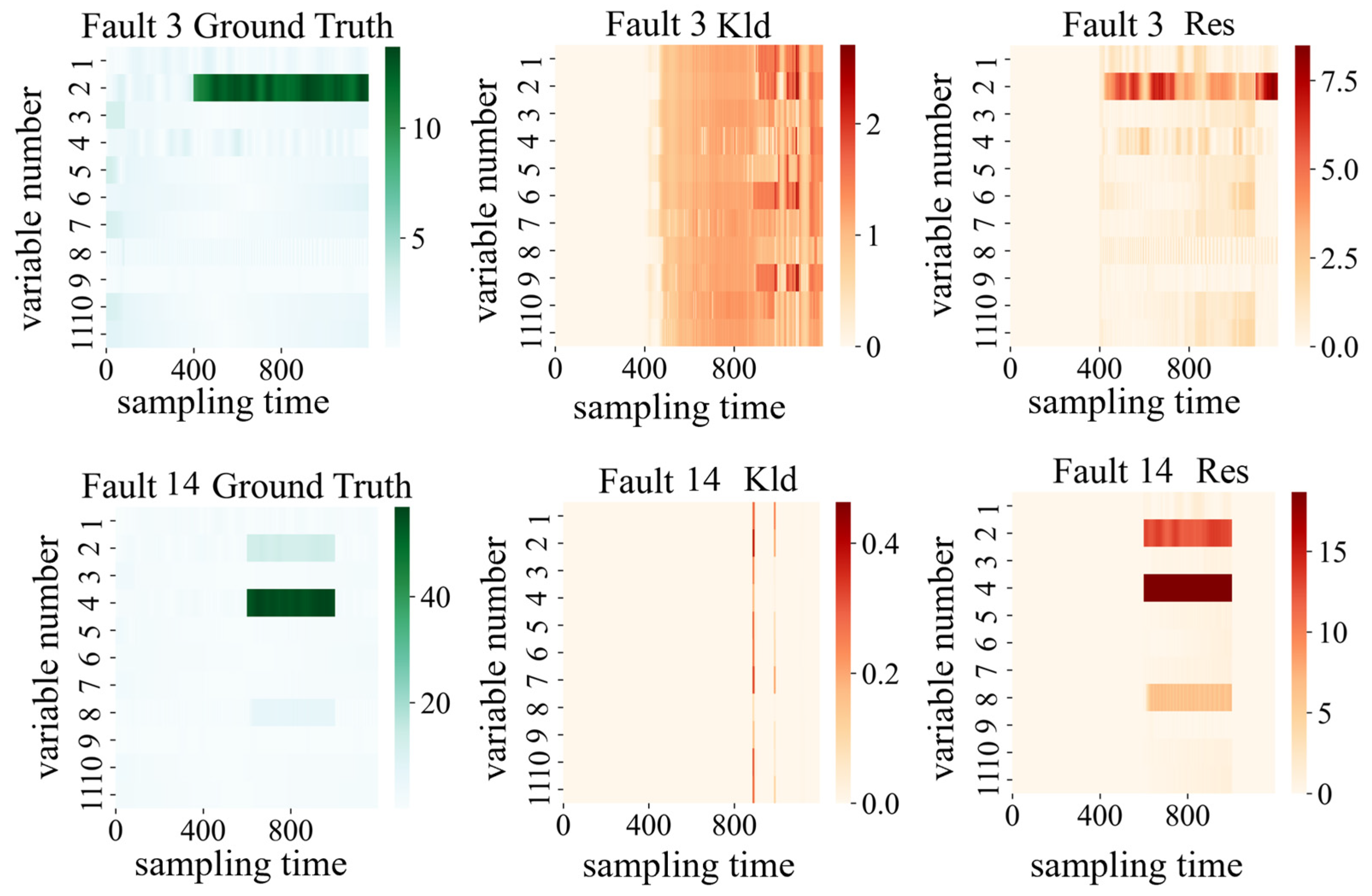
In this section, we use DRBC to locate the root cause of the fault and take fault 3 and fault 14 as examples. Figure 6 is the ground truth and diagnosis results of faults 3 and 14. The horizontal axis of the subgraphs denotes the sampling time, and the vertical axis indicates the variable number. The colors in the subfigure represent the offset amplitude of the fault variable.
Fault 3 is the agitator power (fault number 2) failing at the time of 400 samples to 1200 samples. Comparing the ground truth of fault 3 with the diagnosis results of DRBC in the residual space and latent space, it can be seen that the fault root cause is not accurately located in the shallow space due to the small weight of the shallow space setting; however, the diagnosis results of the residual space obtain ideal diagnostic results. Firstly, the diagnostic results in the residual space show that the variable of fault variable number 2 is faulty, i.e., the stirring power; at the same time, the fault diagnosis results show that the fault fails from the 400th to the 1200th sampling time. Similarly, fault 14 is a multivariable fault with fault variables numbered 2, 4, and 8, corresponding to the agitation power, pH, and substrate feed temperature, respectively. The detection results of fault 14 in the residual space accurately locate the root cause of the fault, and the brightness of the color corresponding to each fault variable corresponds to the degree of fault deviation of each variable.
4.2. The Fed-Batch Fermentation Process of L. plantarum
4.2.1. Process Description
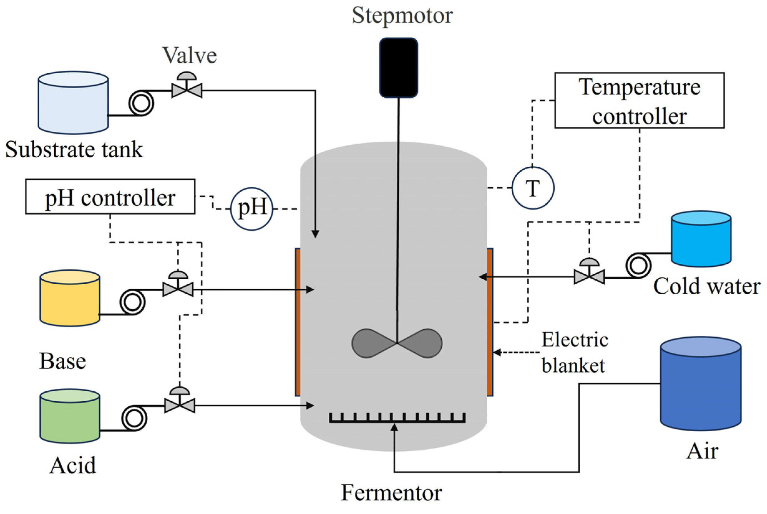
As a kind of lactic acid bacteria that can be used, L. plantarum has the advantages of regulating the human intestine, enhancing immunity, promoting digestion, and regulating antioxidants. The fermentation process of L. plantarum, considered in this work, occupies a significant ratio in the light industrial center. The fermentation equipment is the T&J A-type bioreactor of TJX Bioengineering, and the structure is shown in Figure 7.
The bulk volume of this equipment amounts to 5 L, and sterilization is adopted in an off-site mode. Each fermentation cycle comprises multiple steps. First, the liquid medium needs to be configured. Next, the tank containing liquid medium and three vials filled with supplemental medium, hydrochloric acid, and ammonia are sterilized at 393.15 K for 20 min. After the fermenter is cooled, pre-prepared L. plantarum is added to the fermenter, which marks the beginning of the whole process. Then, the liquid medium is charged into the fermenter after 2 h. The final step is to collect the fermentation product and clean the fermentation tank.
4.2.2. Data Collection and Modeling
In the experiment, we choose the L. plantarum HuNHHMY71L1 as the fermentation strain and refer to the L. plantarum fermentation process in reference [42]. Each batch lasts 8 h, and the sampling interval is set as 1 min. The supplementary medium was added to the medium at 100 mL/min after 2 h. The key variables listed in Table 5 include fermenter temperature, pH, dissolved oxygen, agitation rate, acid supplements, base supplements, and feed supplements.
The 24 batches of data were collected, which included data for 22 batch processes under normal conditions and 2 for typical faults. Under the influence of the cold water flow rate, the temperature will deviate from the normal range, which leads to quality instability. Fault 1: a temperature fault occurred during fermentation, and the temperature was raised by 3 K; and fault 2: the temperature was raised by 0.5 K. The pH was raised by 0.3, and the feeding substrate was delayed by 50 min. The two typical faults are listed in Table 6. The whole fermentation can be divided into three periods according to the turbidity of the fermentation liquid: stage 1: 0–120; stage 2: 120–360; and stage 3: 360–480. The batch-wise and time-wise lag lengths are set to 4 and 8. The weight ratio between the latent and the residual space is set to 1:20. The network structure and training parameters of the CDVAE model for the fermentation process are shown in Table 7.
4.2.3. Fault Detection and Diagnosis of Fault 1 and 2
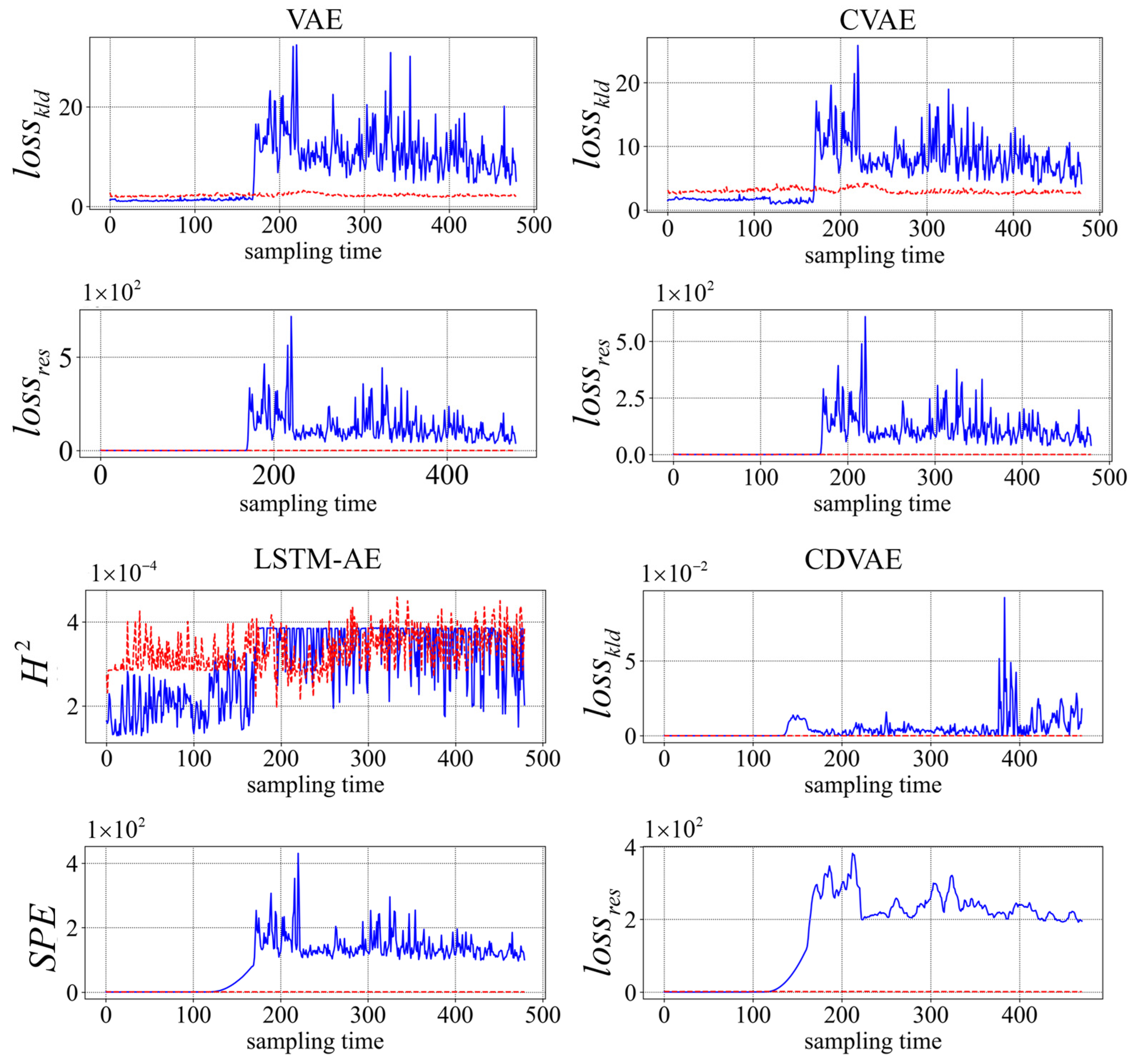
Figure 8 displays the detection plot of fault 2. Obviously, the statistics of the CDVAE model can quickly exceed the control limits and trigger the fault alarm at about the 120th sampling time in both latent and residual spaces, while the statistics of VAE and CVAE exceed the control limit until about the 170th sampling time. Obviously, the detection results of the above two models are not ideal. The LSTM-AE curves in latent space are below the control limit, but the statistic exceeds the control limit at about the 120th sampling time. This also verifies that the fault detection capability of the model has been significantly improved after considering dynamic characteristics.
To further evaluate the overall comparative results of the models for fault detection, the detailed FDR and FAR of each statistic for faults 1 and 2 are shown in Table 8. The proposed model has the highest FDR and lowest FAR compared with other models. The above results fully demonstrate that the proposed model also has good fault detection capabilities in the actual production process.
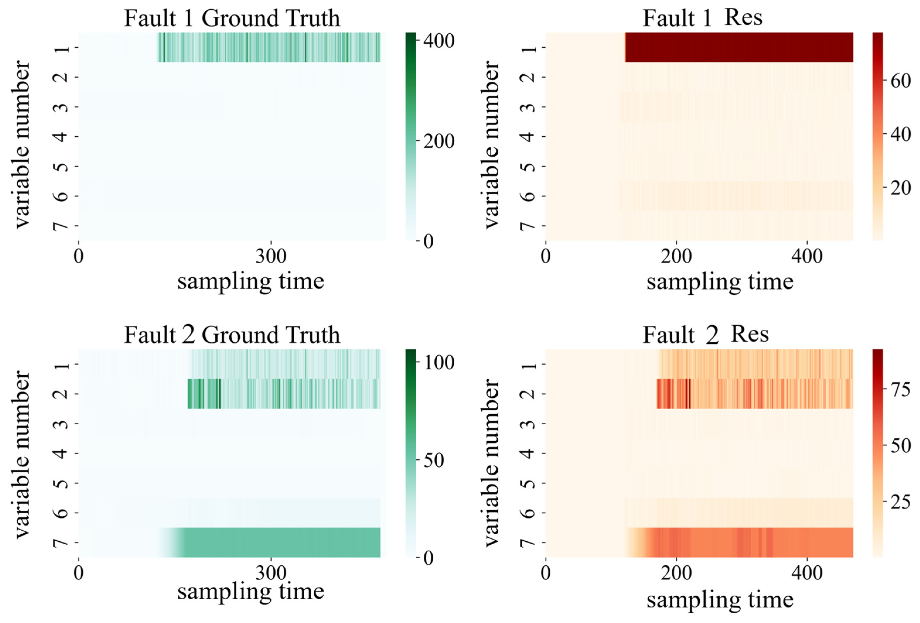
The fault diagnosis of fault 1 and fault 2 is shown in Figure 9. Because the previous diagnostic results in the latent space of the penicillin process were not satisfied, this section only shows the diagnosis results of fermentation process faults in the residual space. The number of iterations for fault diagnosis is set to 5000. Fault 1 is a fermentation temperature fault, and the variable number corresponding to the fault variable is 1. Comparing the diagnosis result of fault 1 in the residual space with the ground truth of fault 1, the diagnosis results of fault 1 can accurately locate the fault variable and time of fault occurrence (120 sampling time). Analyzing the diagnosis results of fault 2 on the residuals, the DRBC-based diagnosis method also located the main variables causing the fault. Therefore, the proposed fault diagnosis algorithm is also effective for multivariable faults in the complex L. plantarum fermentation process.
5. Conclusions
This paper showcased a novel framework integrating a derived model named CVAE and enabling a flexible time-specified threshold for whole-batch process monitoring. The process data are divided into several phases based on batch process historical experience, and then the monitoring is realized by two statistics. The varying control limits can more accurately detect variations in each phase, and a novel method named the DRBC diagram is applied to find and locate the root cause. Applications on the penicillin simulation platform, a real-world fed-batch fermentation process of L. plantarum, indicate that the CDVAE approach performs better than other models. At the same time, the fault diagnosis results on the two data sets show that the DRBC-based diagnosis method can accurately locate the faulty variable and evaluate the fault magnitude.
Author Contributions
Conceptualization, J.Z. and Z.L.; methodology, Z.L., J.Z. and Z.Z.; software, Z.L.; validation, Z.L., Z.Z. and X.L.; formal analysis, X.L.; investigation, J.Z. and Z.L.; resources, J.Z.; data curation, Z.L.; writing—original draft preparation, Z.L., Z.Z. and J.Z.; writing—review and editing, J.Z., Z.Z. and X.L.; visualization, Z.L. and Z.Z.; supervision, F.G.; project administration, J.Z.; funding acquisition, J.Z. All authors have read and agreed to the published version of the manuscript.
Funding
This work was supported by the Natural Science Foundation of Jiangsu Province (Grant No. BK20210452), the National Natural Science Foundation of China (Grant No. 62103168), the Fundamental Research Funds for the Central Universities (JUSRP622034), and the Hong Kong Research Grant Council Project 16203322.
Data Availability Statement
The data presented in this study are available upon request from the corresponding author.
Conflicts of Interest
The authors declare that they have no known competing financial interests or personal relationships that could have appeared to influence the work reported in this paper.
Abbreviations
| Statistical process control | SPC |
| Conditional dynamic variational auto-encoder | CDVAE |
| Principle component analysis | PCA |
| Canonical correlation analysis | CCA |
| Partial least square | PLS |
| Variational auto-encoder | VAE |
| Two-dimensional | 2D |
| Kullback–Leibler divergence | KLD |
| Conditional variational auto-encoder | CVAE |
| Long short-term memory | LSTM |
| Kernel density estimation | KDE |
| Deep reconstruction based on contribution | DRBC |
| Fault detection rate | FDR |
| False alarm rate | FAR |
| Long short-term memory auto-encoder Fully connected layer | LSTM-AE FC |
References
- Wang, K.; Rippon, L.; Chen, J.; Song, Z.; Gopaluni, R.B. Data-driven dynamic modeling and online monitoring for multiphase and multimode batch processes with uneven batch durations. Ind. Eng. Chem. Res. 2019, 58, 13628–13641. [Google Scholar] [CrossRef]
- Joshi, T.; Kodamana, H.; Kandath, H.; Kaisare, N. TASAC: A twin-actor reinforcement learning framework with a stochastic policy with an application to batch process control. Ctrl Eng. Pract. 2023, 134, 105462. [Google Scholar] [CrossRef]
- Fransson, M.; Folestad, S. Real-time alignment of batch process data using COW for on-line process monitoring. Chemom. Intell. Lab. Syst. 2006, 84, 56–61. [Google Scholar] [CrossRef]
- Yoo, H.; Kim, B.; Kim, J.W.; Lee, J.H. Reinforcement learning based optimal control of batch processes using Monte-Carlo deep deterministic policy gradient with phase segmentation. Comput. Chem. Eng. 2021, 144, 107133. [Google Scholar] [CrossRef]
- Md Nor, N.; Che Hassan, C.R.; Hussain, M.A. A review of data-driven fault detection and diagnosis methods: Applications in chemical process systems. Rev. Chem. Eng. 2020, 36, 513–553. [Google Scholar] [CrossRef]
- Ren, L.; Meng, Z.; Wang, X.; Zhang, L.; Yang, L.T. A data-driven approach of product quality prediction for complex production systems. IEEE Trans. Ind. Inform. 2020, 17, 6457–6465. [Google Scholar] [CrossRef]
- Qin, S.J. Survey on data-driven industrial process monitoring and diagnosis. Rev. Chem. Eng. 2012, 36, 220–234. [Google Scholar] [CrossRef]
- Chen, J.; Wei-Yann, W. Performance monitoring of MPCA-based control for multivariable batch control processes. J. Taiwan Inst. Chem. Eng. 2010, 41, 465–474. [Google Scholar] [CrossRef]
- Shen, F.; Zheng, J.; Ye, L.; Ma, X. LSTM soft sensor development of batch processes with multivariate trajectory-based ensemble just-in-time learning. IEEE Access 2020, 8, 73855–73864. [Google Scholar] [CrossRef]
- Gu, S.; Chen, J.; Xie, L. Automatic segmentation of batch processes into multi-local state-space models for fault detection. Chem. Eng. Sci. 2023, 267, 118274. [Google Scholar] [CrossRef]
- de Oliveira, B.N.; Valk, M.; Marcondes Filho, D. Fault detection and diagnosis of batch process dynamics using ARMA-based control charts. J. Process Contr. 2022, 111, 46–58. [Google Scholar] [CrossRef]
- Zhu, J.; Wang, Y.; Zhou, D.; Gao, F. Batch process modeling and monitoring with local outlier factor. IEEE Trans. Contr. Syst. Technol. 2018, 27, 1552–1565. [Google Scholar] [CrossRef]
- Chang, P.; Li, R. Process monitoring of batch process based on overcomplete broad learning network. Eng. Appl. Artif. Intell. 2021, 99, 10413. [Google Scholar]
- Jiang, Q.; Gao, F.; Yan, X.; Yi, H. Multiobjective two-dimensional CCA-based monitoring for successive batch processes with industrial injection molding application. IEEE Trans. Ind. Electron. 2018, 66, 3825–3834. [Google Scholar] [CrossRef]
- Liu, Q.; Zhu, Q.; Qin, S.J.; Chai, T. Dynamic concurrent kernel CCA for strip-thickness relevant fault diagnosis of continuous annealing processes. J. Process Control 2018, 67, 12–22. [Google Scholar] [CrossRef]
- Shi, H.; Kim, M.; Liu, H.; Yoo, C. Process modeling based on nonlinear PLS models using a prior knowledge-driven time difference method. J. Taiwan Inst. Chem. Eng. 2016, 69, 93–105. [Google Scholar] [CrossRef]
- Hao, W.; Lu, S.; Lou, Z.; Wang, Y.; Jin, X.; Deprizon, S. A Novel Dynamic Process Monitoring Algorithm: Dynamic Orthonormal Subspace Analysis. Processes 2023, 11, 1935. [Google Scholar] [CrossRef]
- Yu, W.; Zhao, C. Robust monitoring and fault isolation of nonlinear industrial processes using denoising autoencoder and elastic net. IEEE Trans. Control Syst. Technol. 2019, 28, 1083–1091. [Google Scholar] [CrossRef]
- Qin, S.J.; Zheng, Y. Quality-relevant and process-relevant fault monitoring with concurrent projection to latent structures. AIChE J. 2013, 59, 496–504. [Google Scholar] [CrossRef]
- Agarwal, P.; Aghaee, M.; Tamer, M.; Budman, H. A novel unsupervised approach for batch process monitoring using deep learning. Comput. Chem. Eng. 2022, 159, 107694. [Google Scholar] [CrossRef]
- Agarwal, P.; Gonzalez, J.I.; Elkamel, A.; Budman, H. Hierarchical deep LSTM for fault detection and diagnosis for a chemical process. Processes 2022, 10, 2557. [Google Scholar] [CrossRef]
- Lee, S.; Kwak, M.; Tsui, K.L.; Kim, S.B. Process monitoring using variational autoencoder for high-dimensional nonlinear processes. Eng. Appl. Artif. Intell. 2019, 83, 13–27. [Google Scholar] [CrossRef]
- Yan, W.; Guo, P.; Li, Z. Nonlinear and robust statistical process monitoring based on variant autoencoders. Chemometr. Intell. Lab. Syst. 2016, 158, 31–40. [Google Scholar] [CrossRef]
- Zhang, Z.; Zhu, J.; Ge, Z. Industrial process modeling and fault detection with recurrent Kalman variational autoencoder. In Proceedings of the IEEE 9th Data Driven Control and Learning Systems Conference (DDCLS), Liuzhou, China, 20–22 November 2020. [Google Scholar]
- Zhang, Z.; Jiang, T.; Zhan, C.; Yang, Y. Gaussian feature learning based on variational autoencoder for improving nonlinear process monitoring. J. Process Control 2019, 75, 136–155. [Google Scholar] [CrossRef]
- Zhang, Z.; Zhu, J.; Zhang, S.; Gao, F. Process monitoring using recurrent Kalman variational auto-encoder for general complex dynamic processes. Eng. Appl. Artif. Intell. 2023, 123, 106424. [Google Scholar] [CrossRef]
- Tang, P.; Peng, K.; Dong, J.; Zhang, K.; Jiao, R. A variational autoencoders approach for process monitoring and fault diagnosis. Int. J. Syst. Control Inf. Proc. 2021, 3, 229–245. [Google Scholar] [CrossRef]
- Ren, J.; Ni, D. A batch-wise LSTM-AE decoder network for batch process monitoring. Chem. Eng. Res. Des. 2020, 164, 102–112. [Google Scholar] [CrossRef]
- Qin, S.J.; Li, W. Detection and identification of faulty sensors in dynamic processes. AIChE J. 2001, 47, 1581–1593. [Google Scholar] [CrossRef]
- Zhang, H.; Deng, X.; Zhang, Y.; Hou, C.; Li, C. Dynamic nonlinear batch process fault detection and identification based on two-directional dynamic kernel slow feature analysis. Can. J. Chem. Eng. 2021, 99, 306–333. [Google Scholar] [CrossRef]
- Chang, P.; Ding, C.; Zhao, Q. Fault diagnosis of microbial pharmaceutical fermentation process with non-gaussian and nonlinear coexistence. Chemometr. Intell. Lab. Syst. 2020, 199, 103931. [Google Scholar]
- Jiang, Q.; Yan, S.; Yan, X.; Yi, H.; Gao, F. Data-driven two-dimensional deep correlated representation learning for nonlinear batch process monitoring. IEEE Trans. Ind. Inf. 2020, 16, 2839–2848. [Google Scholar] [CrossRef]
- Wu, S.; Zhang, R. A two-dimensional design of model predictive control for batch processes with two-dimensional (2D) dynamics using extended non-minimal state space structure. J. Process Control 2019, 81, 172–189. [Google Scholar] [CrossRef]
- Yao, H.; Zhao, X.; Li, W.; Hui, Y. Quality-related fault monitoring for multi-phase batch process based on multiway weighted elastic network. Chemometr. Intell. Lab. Syst. 2022, 223, 104528. [Google Scholar] [CrossRef]
- Ye, A.X.; Wang, B.P.; Yang, C.Z. Time sequential phase partition and modeling method for fault detection of batch processes. IEEE Access 2017, 6, 1249–1260. [Google Scholar] [CrossRef]
- Maragathasundari, S.; Eswar, S.K.; Somasundaram, R.S. A study on phases of service and multi-vacation policy in a non-Markovian queuing system. Int. J. Math. Oper. Res. 2022, 21, 444–465. [Google Scholar] [CrossRef]
- Kingma, D.P.; Welling, M. Auto-encoding variational bayes. arXiv 2013, arXiv:1312.6114. [Google Scholar]
- Sohn, K.; Lee, H.; Yan, X. Learning structured output representation using deep conditional generative models. In Proceedings of the Conference and Workshop on NIPS, Montreal, QC, Canada, 7–12 December 2015. [Google Scholar]
- Alcala, C.F.; Qin, S.J. Reconstruction-based contribution for process monitoring. Automatica 2009, 45, 1593–1600. [Google Scholar] [CrossRef]
- Hematillake, D.; Freethy, D.; McGivern, J.; McCready, C.; Agarwal, P.; Budman, H. Design and optimization of a penicillin fed-batch reactor based on a deep learning fault detection and diagnostic model. Ind. Eng. Chem. Res. 2022, 61, 4625–4637. [Google Scholar] [CrossRef]
- Hua, L.; Zhang, C.; Sun, W.; Li, Y.; Xiong, J.; Nazir, M.S. An evolutionary deep learning soft sensor model based on random forest feature selection technique for penicillin fermentation process. ISA Trans. 2023, 136, 139–151. [Google Scholar] [CrossRef]
- Krieger, W.S.; Heras, J.M.; Suarez, C. Lactobacillus plantarum, a new biological tool to control malolactic fermentation: A review and an outlook. Beverages 2020, 6, 2. [Google Scholar] [CrossRef]
Figure 1.
Illustration of the 2D sliding window.

Figure 2.
The structure of the CDVAE.

Figure 3.
Flow chart of the DRBC diagram.

Figure 4.
Scheme of CDVAE process monitoring.

Figure 5.
Fault 3 detection results under VAE, CVAE, LSTM-AE, and CDVAE. (The blue solid line: the statistic, the red dotted line: control limit).
Figure 5.
Fault 3 detection results under VAE, CVAE, LSTM-AE, and CDVAE. (The blue solid line: the statistic, the red dotted line: control limit).

Figure 6.
Fault diagnosis results for faults 3 and 14.

Figure 7.
Structure of the fermentation process.

Figure 8.
Fault 2 detection results under VAE, CVAE, LSTM-AE, and CDVAE. (The blue solid line: the statistic, the red dotted line: control limit).
Figure 8.
Fault 2 detection results under VAE, CVAE, LSTM-AE, and CDVAE. (The blue solid line: the statistic, the red dotted line: control limit).

Figure 9.
Fault diagnosis results for faults 1 and 2.


Table 1.
The variables of the penicillin fermentation process.
| No. | Variables | Unit |
|---|---|---|
| 1 | Aeration rate | L/h |
| 2 | Agitator power | W |
| 3 | Substrate feed rate | L/h |
| 4 | Substrate feed temperature | K |
| 5 | Substrate concentration | g/L |
| 6 | Dissolved oxygen concentration | g/L |
| 7 | Biomass concentration | g/L |
| 8 | Culture volume | L |
| 9 | Carbon dioxide concentration | g/L |
| 10 | pH | / |
| 11 | Fermenter temperature | K |
Table 2.
Parameters of the CDVAE model for penicillin simulation data.
| Description | Value | |
|---|---|---|
| CDVAE | Encoder network: (, ) → | LSTM (10)→FC (800 + 3)→FC (400)→FC (3) |
| Decoder network: (, ) → | LSTM (3)→FC (400 + 3)→FC (800)→FC (300) | |
| Learning rate | 0.001 | |
| Activate function | “Leaky_Relu” | |
| Training epochs | 500 | |
| Batch size of training samples | 128 |
Table 3.
Description of different types of faults.
| No. | Fault Variables | Magnitude | Fault Type | Start Sampling Time | End Sampling Time |
|---|---|---|---|---|---|
| 1 | Agitator power | 2% | Step | 400 | 1200 |
| 2 | Agitator power | 3% | Step | 400 | 1200 |
| 3 | Agitator power | 5% | Step | 400 | 1200 |
| 4 | pH | −2% | Step | 400 | 1200 |
| 5 | pH | −3% | Step | 400 | 1200 |
| 6 | Substrate feed rate | +0.005 L/h | Ramp | 400 | 1200 |
| 7 | Substrate feed rate | −0.01 L/h | Ramp | 400 | 1200 |
| 8 | Aeration rate | −1% | Step | 400 | 1200 |
| 9 | Aeration rate | +2% | Step | 400 | 1200 |
| 10 | Aeration rate | −3% | Step | 400 | 1200 |
| 11 | Aeration rate | +0.02 L/h | Ramp (saturate at 5 L/h) | 400 | 700 |
| 12 | Aeration rate | −0.02 L/h | Ramp (saturate at 5 L/h) | 400 | 700 |
| 13 | Agitator power/pH/ Substrate feed temperature | +5%/+5%/+3% | Step | 600 | 1000 |
| 14 | Agitator power/pH/Substrate feed temperature | +5%/−5%/−3% | Step | 600 | 1000 |
Table 4.
Fault detection results of different faults under VAE, CVAE, LSTM-AE, and CDVAE (%).
| No. | VAE | CVAE | LSTM-AE | CDVAE | ||||||||
|---|---|---|---|---|---|---|---|---|---|---|---|---|
| losskld | lossres | FAR | losskld | lossres | FAR | H2 | SPE | FAR | losskld | lossres | FAR | |
| 1 | 14.0 | 87.3 | 1.5 | 38.5 | 79.2 | 1.1 | 25.6 | 87.8 | 0.42 | 94.3 | 94.7 | 0.12 |
| 2 | 20.3 | 98.5 | 1.7 | 46.5 | 96.3 | 1.2 | 42.3 | 98.3 | 0.35 | 100 | 100 | 0.13 |
| 3 | 41.3 | 100 | 1.6 | 61.4 | 100 | 0.87 | 83.1 | 100 | 0.25 | 100 | 100 | 0.07 |
| 4 | 7.0 | 9.6 | 0.9 | 11.8 | 12.1 | 0.75 | 14.5 | 24.8 | 0.12 | 9.3 | 54.4 | 0.15 |
| 5 | 9.3 | 48.8 | 1.5 | 7.8 | 46.3 | 0.75 | 23.1 | 73.3 | 0.02 | 16.4 | 90.1 | 0.25 |
| 6 | 6.1 | 4.4 | 1.7 | 27.1 | 11.0 | 0.85 | 3.7 | 49.6 | 0.24 | 55.8 | 59.1 | 0.00 |
| 7 | 13.4 | 17.6 | 2.1 | 9.0 | 16.5 | 0.75 | 49.6 | 18.4 | 0.48 | 52.6 | 17.5 | 0.00 |
| 8 | 28.5 | 31.1 | 2.0 | 48.1 | 40.7 | 0.72 | 53.6 | 66.5 | 0.25 | 67.2 | 89.6 | 0.70 |
| 9 | 78.6 | 89.7 | 1.7 | 32.9 | 96.6 | 0.85 | 84.6 | 97.5 | 1.12 | 87.4 | 100 | 0.51 |
| 10 | 93.5 | 97.3 | 2.1 | 72.4 | 100 | 1.35 | 96.4 | 100 | 0.89 | 100 | 100 | 0.30 |
| 11 | 88.7 | 97.67 | 1.8 | 87.3 | 96.3 | 1.23 | 96.3 | 96.6 | 0.25 | 91.7 | 98.7 | 0.00 |
| 12 | 84.1 | 98.34 | 1.7 | 95.7 | 95.7 | 1.24 | 95.0 | 98 | 0.12 | 99.0 | 100 | 0.00 |
| 13 | 95.5 | 100 | 2.3 | 100 | 100 | 1.34 | 95.3 | 100 | 1.12 | 100 | 100 | 0.80 |
| 14 | 100.0 | 100 | 1.8 | 100 | 100 | 1.76 | 95.3 | 100 | 0.85 | 100 | 100 | 0.30 |
| Average | 48.6 | 70.7 | 1.7 | 52.7 | 70.8 | 1.0 | 61.0 | 79.2 | 0.46 | 73.84 | 86.01 | 0.23 |
Table 5.
The key variables of the batch fermentation process.
| No. | Variable | Unit |
|---|---|---|
| 1 | Fermenter temperature | K |
| 2 | pH | / |
| 3 | Dissolved oxygen | / |
| 4 | Agitation rate | r/min |
| 5 | Acid supplements | mL |
| 6 | Base supplements | mL |
| 7 | Feed supplements | mL |
Table 6.
Faults description of the fermentation process.
| No. | Fault Variables | Magnitude | Fault Type | Start Sampling Time | End Sampling Time |
|---|---|---|---|---|---|
| 1 | Fermentation temperature | +3 K | Step | 120 | 480 |
| 2 | Fermentation temperature/ pH/Feed supplement | +0.5 K/ +0.3/50 min Delay | Step | 120 | 480 |
Table 7.
Parameters of the CDVAE model for fermentation process data.
| Description | Value | |
|---|---|---|
| CDVAE | Encoder network: (, ) → | LSTM (6)→FC (400 + 3)→FC (200)→FC (3) |
| Decoder network: (, ) → | LSTM (3)→FC (200 + 3)→FC (400)→FC (192) | |
| Learning rate | 0.001 | |
| Activate function | “Leaky_Relu” | |
| Training epochs | 1000 | |
| Batch size of training samples | 128 |
Table 8.
Fault detection results under VAE, CVAE, LSTM-AE, and CDVAE (%).
| No. | VAE | CVAE | LSTM-AE | CDVAE | ||||||||
|---|---|---|---|---|---|---|---|---|---|---|---|---|
| losskld | lossres | FAR | losskld | lossres | FAR | H2 | SPE | FAR | losskld | lossres | FAR | |
| 1 | 99.1 | 97.2 | 3.8 | 97.5 | 98.8 | 3.0 | 26.3 | 98.3 | 0.6 | 99.7 | 99.7 | 0.0 |
| 2 | 84.1 | 87.5 | 5.1 | 83.6 | 91.6 | 3.5 | 51.1 | 97.5 | 0.5 | 100 | 100 | 0.0 |
Disclaimer/Publisher’s Note: The statements, opinions and data contained in all publications are solely those of the individual author(s) and contributor(s) and not of MDPI and/or the editor(s). MDPI and/or the editor(s) disclaim responsibility for any injury to people or property resulting from any ideas, methods, instructions or products referred to in the content. |
© 2024 by the authors. Licensee MDPI, Basel, Switzerland. This article is an open access article distributed under the terms and conditions of the Creative Commons Attribution (CC BY) license (https://creativecommons.org/licenses/by/4.0/).
Share and Cite
MDPI and ACS Style
Zhu, J.; Liu, Z.; Lou, X.; Gao, F.; Zhang, Z. Time-Specific Thresholds for Batch Process Monitoring: A Study Based on Two-Dimensional Conditional Variational Auto-Encoder. Processes 2024, 12, 682. https://doi.org/10.3390/pr12040682
AMA Style
Zhu J, Liu Z, Lou X, Gao F, Zhang Z. Time-Specific Thresholds for Batch Process Monitoring: A Study Based on Two-Dimensional Conditional Variational Auto-Encoder. Processes. 2024; 12(4):682. https://doi.org/10.3390/pr12040682
Chicago/Turabian StyleZhu, Jinlin, Zhong Liu, Xuyang Lou, Furong Gao, and Zheng Zhang. 2024. "Time-Specific Thresholds for Batch Process Monitoring: A Study Based on Two-Dimensional Conditional Variational Auto-Encoder" Processes 12, no. 4: 682. https://doi.org/10.3390/pr12040682
Note that from the first issue of 2016, this journal uses article numbers instead of page numbers. See further details here.