Computational Ensemble Gene Co-Expression Networks for the Analysis of Cancer Biomarkers

Abstract

Gene networks have become a powerful tool for the comprehensive examination of gene expression patterns. Thanks to these networks generated by means of inference algorithms, it is possible to study different biological processes and even identify new biomarkers for such diseases. These biomarkers are essential for the discovery of new treatments for genetic diseases such as cancer. In this work, we introduce an algorithm for genetic network inference based on an ensemble method that improves the robustness of the results by combining two main steps: first, the evaluation of the relationship between pairs of genes using three different co-expression measures, and, subsequently, a voting strategy. The utility of this approach was demonstrated by applying it to a human dataset encompassing breast and prostate cancer-associated stromal cells. Two gene networks were computed using microarray data, one for breast cancer and one for prostate cancer. The results obtained revealed, on the one hand, distinct stromal cell behaviors in breast and prostate cancer and, on the other hand, a list of potential biomarkers for both diseases. In the case of breast tumor, ST6GAL2, RIPOR3, COL5A1, and DEPDC7 were found, and in the case of prostate tumor, the genes were GATA6-AS1, ARFGEF3, PRR15L, and APBA2. These results demonstrate the usefulness of the ensemble method in the field of biomarker discovery.

1. Introduction

The incidence rates of breast and prostate cancer are among the highest among women and men, respectively. The number of breast cancer cases is expected to increase from 2.3 million in 2020 to over 3 million by 2040 [1], while prostate cancer cases will double from 1.4 million to 2.8 million during the same period [2]. Despite improvements in therapeutic strategies, it remains essential to increase our understanding of the mechanisms underlying cancer progression and to identify new targets for cancer therapy, such as molecules in the tumor microenvironment (TME). The TME plays a key role in tumor growth, development, and progression and includes different cell types, including stromal cells. Stromal cells and their associated components, such as the extracellular matrix (ECM), interact with cancer cells to create a permissive microenvironment that supports cancer progression and may even serve as potential biomarkers for cancer research [3,4,5,6]. However, it is essential to keep in mind that the tumor stromal is not a static entity but a dynamic and constantly changing one. Therefore, to better understand the functions and mechanisms by which stromal components and their interactions with tumor cells drive cancer initiation and progression, it is necessary to identify potential biomarkers.

For the discovery of diagnostic, prognostic, and predictive biomarkers for diseases such as cancer, as well as for testing the efficacy of potential therapeutic agents, sequencing technologies such as RNA-Seq, microarrays, and single-cell sequencing have become essential tools [7]. These technologies allow comprehensive analysis of the genetic profile, gene expression, and gene–gene interactions when computational (in-silico) approaches are used to analyze these data. These computational approaches, such as gene co-expression networks (GCNs), can enhance this analysis using the data generated by sequencing technologies to predict and model gene–gene interactions. This can facilitate the understanding of biological processes and help identify biomarkers involved in different diseases [8].

GCNs depict the relationship between genes using a graph, in which the vertices represent the genes and the edges represent their relationship. These relationships exhibit similar patterns of expression. For a relationship to be deemed significant, the degree of relationship between each pair of genes must surpass a minimum threshold of required expression pattern similarity. Common methods for measuring the degree of co-expression between two genes include Pearson’s, Spearman’s, and Kendall’s correlation coefficients [9]. For the reconstruction of the GCN, mutual information and other methods have also been extensively employed [10]. The development of hypotheses has been aided by GCN models validated through empirical methodologies. Thus, the dependability of GCNs is supported by the subsequent experimental confirmation of numerous predicted interactions [11]. As a result, algorithms and computational techniques for GCN reconstruction have gained prominence within the bioinformatics community [12].

In this context, the traditional methods for reconstructing GCNs using one of these correlation coefficients frequently have the drawback that the inference of gene–gene interactions is wholly dependent on the results of the selected correlation coefficient. For instance, the weighted gene co-expression network analysis (WGCNA) method allows the construction of a network utilizing the Pearson correlation coefficient [13], whereas Spearman is used in another GCN reconstruction method [14]. It is common knowledge that these correlation coefficients have certain limitations, such as the degree of dependence on the normalization of the data in the Pearson coefficient [15] or the inability of the Spearman coefficient to obtain monotonic relationships [16]. The use of a single correlation coefficient in GCN reconstruction methodologies may therefore produce unreliable results, as significant relationships may exist even if one of these correlation coefficients has a value of zero. In order to overcome these limitations, the combination of multiple correlation coefficients to measure the degree of gene–gene interaction may help to improve the reliability of the results and provide more accurate biological information by overcoming the individual limitations of the coefficients [17].

This paper presents a study for the identification of candidate biomarkers for breast and prostate cancer using an ensemble co-expression network algorithm. The expression data used were obtained from stromal tissue within the respective tumor microenvironments. The algorithm applied to infer gene networks consists of an ensemble strategy combining three widely used correlation coefficients, in order to classify gene–gene interactions. As a result, a network was generated from stromal tissue surrounding invasive primary breast and prostate tumors and compared with another network generated from non-cancerous breast and prostate stromal tissues. Cross-analysis of these networks provided significant information on the biological functions affected in both situations, helping to identify potentially novel breast and prostate carcinoma biomarkers.

The main contributions of this work can be summarized as follows:

• We propose a case study based on three different widely GCN-inferred algorithms.
• The use of the ensemble strategy derives from a more reliable inferred GCN.
• A case study of breast and prostate cancer is presented.
• We propose several genes as potential biomarkers for both breast and prostate cancers.

The rest of the paper is organized as follows: The main related works are presented in Section 1. The datasets and the case study used are detailed in Section 2. The results related to the generation and analysis of the GCNs are described in Section 3, while the discussion of the work is presented in Section 4. Finally, the conclusions are given in Section 5.

Related Works

GCNs have emerged as a useful instrument for data analysis and the discovery of new biomarkers. For instance, despite a high computational cost as a result of its reliance on permutation tests to determine significance [18], the WGCNA method [13] is widely used, as highlighted in studies such as Tang et al. [19] in metastatic breast cancer, identifying key modules and core genes. In addition, Zhou et al. [20], Adhami et al. [21], and Ye [22] found biomarkers associated with breast cancer progression and subtypes. In prostate cancer, WGCNA was also used by the authors in Song et al. [23], Xu et al. [24], and Liu et al. [25] to identify key genes and biomarkers for diagnosis and prognosis.

Other works related to the identification of biomarkers for breast and prostate cancer have used other methods or networks. Protein–protein interaction (PPI) networks have been used to determine that the mitotic cell cycle and the epithelial-to-mesenchymal transition pathway are associated with breast cancer progression [26]. The authors Hsu et al. [14] discovered that integration between gene co-expression network analysis (GCNA) and integrated microarray analysis [27] can yield more accurate diagnoses. The ARACNE network reconstruction method [28] has also been used to identify drug targets to advance the treatment of prostate cancer patients [29].

Inferring gene–gene relationships can be hampered by the reliance on works that employ a single network reconstruction method or a single correlation coefficient. One solution to this problem is the development of new ensemble strategies. In one work, for instance, the authors used a combination of methods to infer with high confidence connections between dynamically active factors [30]. Their strategy employed the following methods: PLSR [31], similarity index [32], TIGRESS [33], random forest [34], ARACNE, CLR [35], and MRNET [36]. The studies conducted by Hsu et al. [14] in breast cancer and Ferraz et al. [37] in prostate cancer demonstrated that the combination of methodologies and correlation measures improved the robustness of the results. In another work, the authors chose to implement an ensemble strategy at the level of co-expression measures, as opposed to the level of methods [17]. The correlation between each deferentially expressed gene–gene interaction was determined using Pearson’s, Kendall’s, and Blomqvist’s correlation coefficients. This ensemble strategy reconstructed two GCNs, one corresponding to the cancer state and the other to the normal state, which could be used as a control network for further gene analysis. The EnGNet approach [38] was another work that employed an ensemble strategy to generate gene co-expression networks. The co-expression network was generated using Spearman, Kendall, and NMI correlation measurement combinations and then optimized using a greedy approach.

In summary, the preceding works highlighted the importance of GCNs in breast and prostate cancer biomarker discovery. While the use of WGCNA in breast and prostate cancer research has yielded promising results, there has been a trend towards the diversification of network analysis methodologies. The use of alternative network types and correlation coefficients increases the robustness of results, ensuring that the identified biomarkers are not artifacts of a particular method or dataset. Indeed, relying on a single network reconstruction technique or correlation coefficient can lead to biased results and make it difficult to identify gene–gene relationships with precision. Ensemble strategies, which utilize a variety of correlation methods and measurements, have emerged as a viable response to this situation. These strategies ensure that connections between dynamically active factors are inferred with a high degree of confidence, thereby contributing to the more precise identification of potential biomarkers and cancer treatment targets.

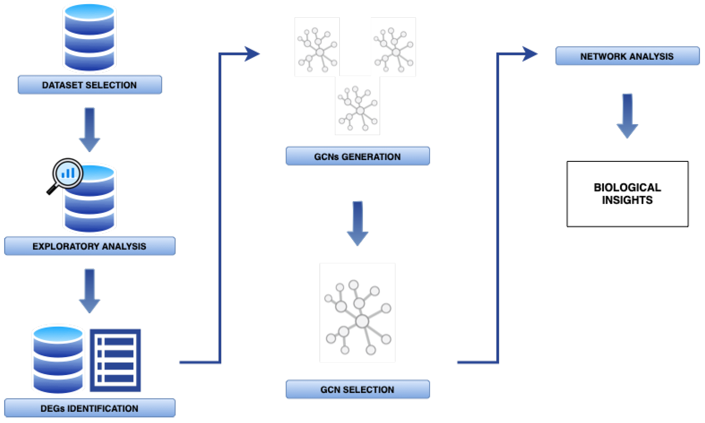
2. Materials and Methods

This section describes the dataset used and outlines the subsequent stages of the analysis. Specifically, the microarray dataset came from research on breast and prostate cancer. Additionally, the workflow used to carry out the study (depicted in Figure 1) is also detailed in the following subsections, as follows: First, the employed dataset is described in Section 2.1, followed by the exploratory analysis performed on the expression data in Section 2.2. Subsequently, Section 2.3 provides an explanation of the differential expression analysis; the method used for GCN reconstruction and candidate GCN selection is described in Section 2.4 and Section 2.5, respectively. Finally, in Section 2.6, the analysis of GCNs is conducted. Figure 1 depicts the entire pipeline, including all the previously mentioned steps.

2.1. Sample Dataset

The microarray dataset used in this study was published by Planche et al. [39]. It was obtained from the National Centre of Biotechnology Information (NCBI) Gene Expression Omnibus (GEO) database with the accession number GSE26910. The gene profiling data were obtained using the Affymetrix Human Genome U133 Plus 2.0 Array (Platform GPL570). The dataset contained 24 samples, including 6 samples of stroma surrounding invasive breast primary tumors, 6 matching samples of normal stromal breast tissues, 6 samples of stroma surrounding invasive prostate primary tumors, and 6 matching samples of normal stromal prostate tissues, for a total of 20,824 genes. The breast and prostate data were provided by the authors as raw CEL files and normalized with the RMA algorithm (quantile normalization at probe level data).

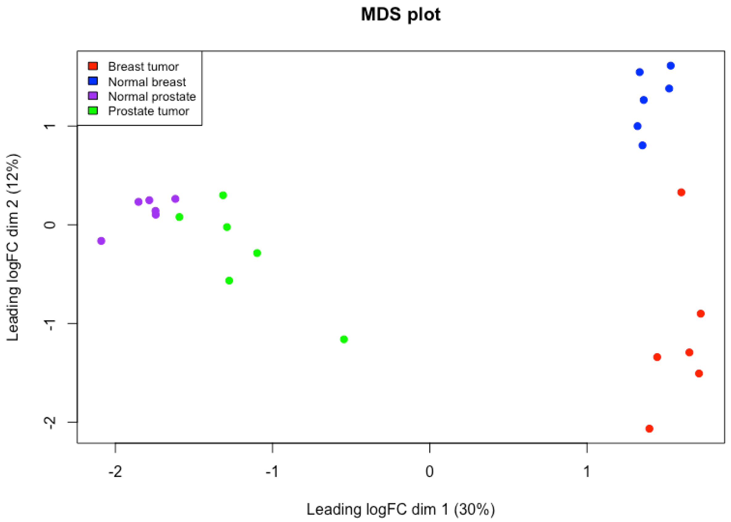
2.2. Data Preprocessing and Exploratory Analysis

A preliminary exploratory analysis was carried out with the aim of obtaining an initial and detailed understanding of the data to be analyzed. This prior exploratory analysis of the expression data obtained from the dataset aimed to identify the quality of the data, detect patterns and trends, as well as determine their distribution. To carry out this analysis, the R programming language was employed. Multidimensional scaling plots (MDS) were applied to further separate examples according to their features. The R plotMDS function was used from the Limma package [40].

The next step involved examining whether the data had been correctly normalized after applying the RMA algorithm. This is crucial to obtaining accurate and reliable results in gene expression analysis because it guarantees the comparability of gene expression values between samples. The R function boxplot was used for this purpose [41].

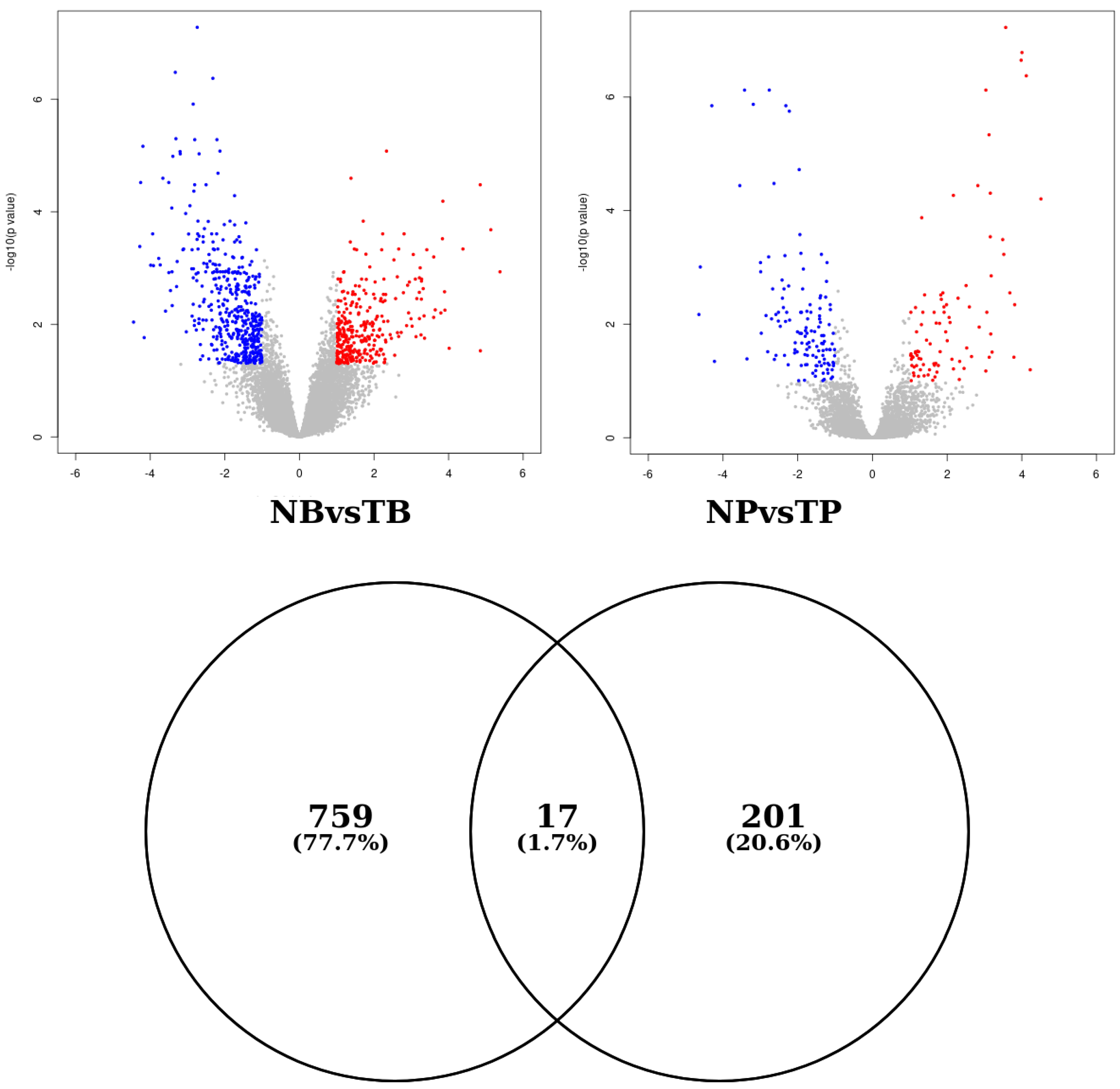
2.3. Differential Gene Expression Analysis

Differential expression analysis is a statistical technique that enables the investigation of normalized data, to identify quantitative alterations in the expression levels between different samples. The primary objective of this task was to identify the genes that show differential expression in our sample sets. This filter is crucial to the analysis of pathologically relevant genes. The samples were grouped into two categories for analysis, male and female, resulting in two sets of differentially expressed genes (DEGs).

The Limma [40] R package was also employed to execute this task, which involved several steps. First, a design matrix was created in our study to specify the contrasts of interest. Specifically, these contrasts were defined as the comparison of normal tissue against tissue derived from cancer patients, both male and female. A linear model was fitted to the expression values of each gene, and empirical Bayes moderation was carried out by borrowing information across all the genes to obtain more precise estimates of gene-wise variability [42]. Subsequently, genes that exhibited statistically significant changes in their expression levels, significantly upregulated or downregulated (with FC > 1 and FC <−1), were detected. This involved determining a threshold for statistical significance based on an adjusted p-value, which was set to 5% for breast stromal samples and 10% for prostate stromal samples to obtain a list of DEGs of comparable size, as explained in Planche et al. [39].

After identifying the DEGs in both prostate and breast tissues, we generated four distinct datasets from the log2-transformed DEG data. These four datasets represented the gene expression profiles of normal prostate, prostate tumor, normal breast, and breast tumor samples.

From the DEGs generated for breast and prostate, respectively, four datasets were produced: normal breast, tumor breast, normal prostate, and tumor prostate, containing the DEGs with symbol correspondence for the Affy names, no duplicates, and the different samples for each condition.

2.4. Gene Co-Expression Network Reconstruction

In this section, the proposed method for ensemble GCNs is introduced. For the generation of GCNs, an algorithm was developed in Python. The algorithm used comprised two main steps: evaluation of the relationship between each gene pair based on three different co-expression measures, followed by a major voting strategy. As a result, the final co-expression network exhibited more reliable interactions and sparseness than other techniques that adopt single co-expression measurements.

In the first phase, the algorithm made an evaluation of the gene–gene relationship using three different evaluation measures. The co-expression measures used for this task were Pearson’s, Spearman’s, and Kendall’s coefficients [43,44]. This choice was motivated by the following observations: The Pearson coefficient is widely used to test dependencies between gene expression levels. It allows us to quantify the strength of the linear relationship between two variables, which in this case corresponds to the expression level of each gene that is being compared. The Spearman coefficient does not require assumptions of linearity in the relationship between variables. Thus, it can identify monotonic relationships between pairs of genes, meaning that as the expression level of one gene increases, so does the expression level of the other, but not necessarily at a constant rate. This property makes it particularly useful for capturing complex relationships between genes that are not strictly linearly correlated. Finally, the Kendall measure evaluates the degree of strength of monotonic relationships. However, it differs in that it is a non-parametric measure, which implies that it does not necessitate an assumption about the distribution of the genes expression levels being compared, making it more robust to outliers and non-normality.

The Python SciPy.stats library was used to evaluate the correlation values of each gene pair using the correlation coefficients contained in the stats subpackage [45].

• Pearson’s correlation coefficient: The values of Pearson’s correlation coefficient range from −1 to 1, with a score of −1 indicating a perfectly negative correlation, a score of 1 indicating a perfectly positive correlation, and a score of 0 indicating no correlation between the expression levels of the two genes under consideration.

  $$\rho =\frac{\sum (x_i-\overline{x})(y_i-\overline{y})}{\sqrt{\sum {(x_i-\overline{x})}^2}\sqrt{\sum {(y_i-\overline{y})}^2}}$$

  where $\rho$ refers to Pearson’s correlation value between gene x and gene y.
• Spearman’s correlation coefficient: The values of Spearman’s correlation coefficient range from −1 to 1, as in the case of Pearson’s.

  $$\rho =1-\frac{6\sum d_i^2}{n(n^2-1)}$$

  where $\rho$ refers to Spearman’s correlation value, $d^2$ to the differences between the ranks of x and y and n to the number of observations.
• Kendall’s correlation coefficient: this coefficient ranges from −1 to 1 and represents a valuable parameter for detecting non-linear relationships among genes.

  $$\tau =\frac{n_c-n_d}{\frac{1}{2}n(n-1)}$$

  where $\tau$ refers to Kendall’s correlation value, $n_c$ to the number of concordant pairs of observations and $n_d$ to the number of discordant pairs of observations.

Upon calculation of the three correlation measurements for each pair of genes, a correlation threshold was established.

The final significance assessment was carried out through a voting system, wherein a relationship between a pair of genes was considered significant if two of the three correlation values exceeded a chosen threshold [38]. Hence, a relationship was added to the final co-expression network if it was considered correct.

Multiple co-expression networks were constructed for each group of deferentially expressed genes using varying threshold values. A total of 20 networks were generated by applying threshold values ranging from 0.7 to 0.9. Specifically, we constructed five co-expression networks using gene expression data from stromal tissue surrounding invasive primary breast tumors, another five networks from normal breast stroma, five networks from gene expression data derived from stromal tissue surrounding invasive primary prostate tumors, and the last five networks from normal prostate stroma.

2.5. Candidate Gene Co-Expression Network Selection

This section outlines the process employed to select the most suitable GCNs for further analysis. To evaluate the GCNs from the different thresholds, we employed the Cytoscape GNC-app [46] to calculate the gene network coherence (GNC) value. This software leverages network representations of biological databases to evaluate the biological coherence of the selected GCNs. In this study, BioGrid (human) served as the reference network for our analysis because it is a repository of biomedical interaction data that have been meticulously curated [47]. It is crucial to note that, during this evaluation, the co-expression networks were not explicitly filtered against the BioGrid network.

For this purpose, a mathematical formula was derived (obtaining a value called $Th{r}_{score}$). The $Th{r}_{score}$ provided the corresponding value, representing the percentage by which the GNC value decreased per deleted edge concerning the network generated with the preceding lower threshold. Upon reaching minimal values, this indicated that the removed edges made minimal contributions to the GNC value in comparison to the prior network. Consequently, it became feasible to select this network for further analysis.

$$Th{r}_{score}=\frac{\%\mathrm{decrease}\mathrm{in}\mathrm{GNC}\mathrm{value}}{\mathrm{number}\mathrm{of}\mathrm{eliminated}\mathrm{edges}\mathrm{concerning}\mathrm{the}\mathrm{prior}\mathrm{network}}$$

With the above, it is important to note that the threshold with the lowest $Th{r}_{score}$ value was the one selected for network generation.

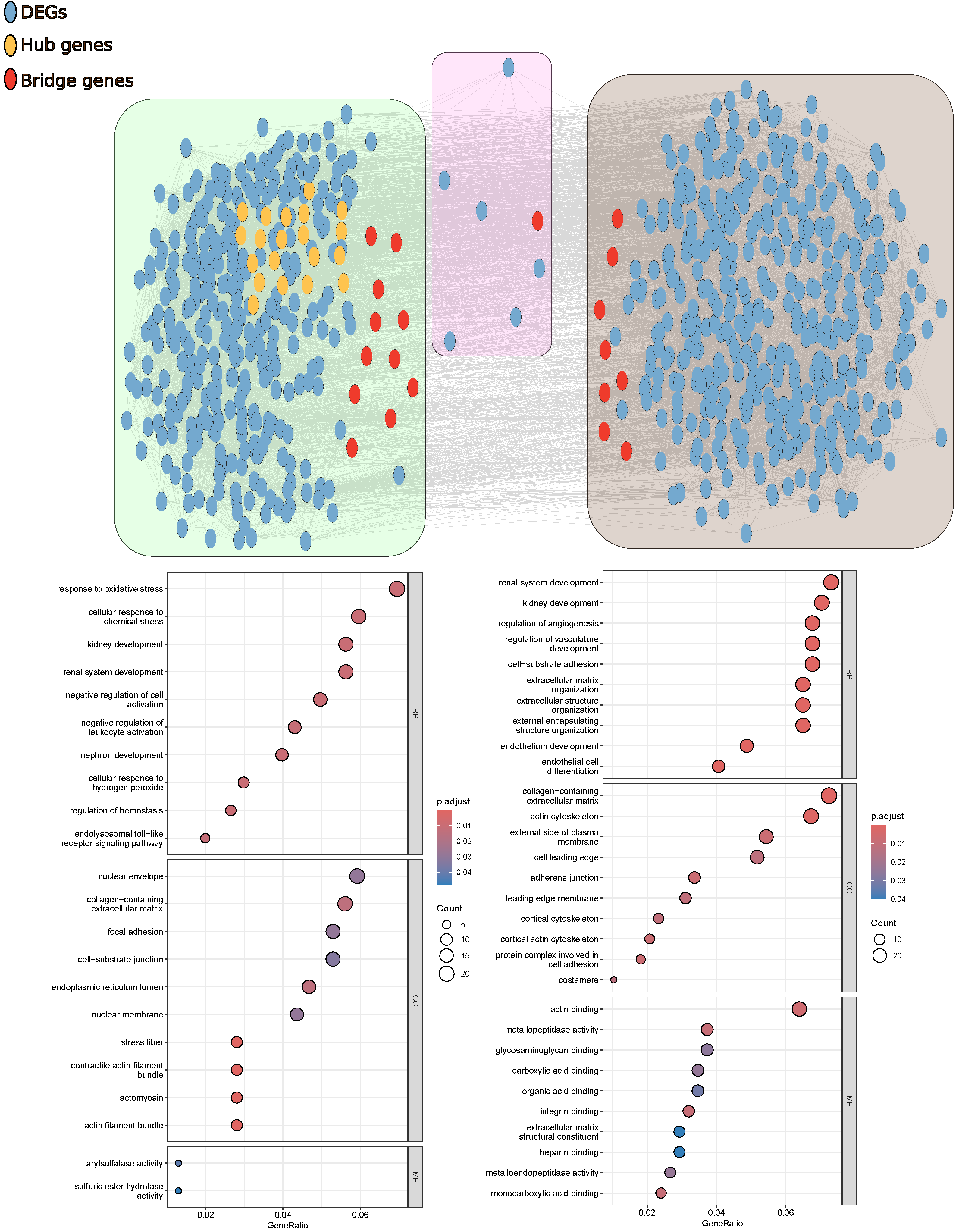
2.6. Gene Co-Expression Network Analysis

The final GCNs, upon which the topological analysis was conducted, were derived through the juxtaposition of network values for GNC [48], nodes, and interactions. A unique cancer-specific network was derived by excluding shared interactions between normal and tumor samples and exclusively retaining interactions specific to the tumor context in breast and prostate cases. The final collection of GCNs for breast and prostate was carried out in the R programming language.

In order to examine the selected co-expression networks, topological and enrichment analyses were conducted. The topological analysis entailed the identification of hubs and clustering, followed by an enrichment analysis of the clusters generated within each co-expression network. In a GCN, hubs are highly connected nodes that have a large number of edges or connections with other nodes and may be considered key components of the co-expression network [49].

Hub genes were selected using Cytoscape software named CytoHubba according to the degree algorithm [50]. This method calculates the degree of connectivity of each node within the co-expression network and ranks them according to this value. The top 20 hub genes were filtered.

Clustering evaluation was performed in order to identify densely connected nodes. The clustering method used was community clustering (GLay) [51], implemented through Cytoscape’s ClusterMaker app [52].

The gene ontology (GO) [53,54] and KEGG [55] enrichment analyses carried out on the previously generated gene clusters were performed using the clusterProfiler [56] R package for comparing biological themes among gene clusters.

3. Results

The generation and analysis of GCNs implemented for this study involved a variety of stages that are described in detail in the following sections. Specifically, Section 3.1 illustrates the exploratory analysis conducted on the dataset used, while Section 3.2 identifies the DEGs. Section 3.3 uses the GNC metric to assess and compare the coherence of the results with other GCN methods and to determine the best threshold. The succeeding Section 3.4 undertakes network reconstruction and selection. Finally, the analysis of the candidate co-expression networks for stromal tissues corresponding to both breast and prostate in a tumor context is performed in Section 3.5.

The primary objective of this study was to identify novel biomarkers through the creation and comprehensive analysis of co-expression networks. To construct these co-expression networks, we employed an algorithm that assessed the associations between gene pairs using three distinct co-expression measures, subsequently employing a majority voting strategy. This case study was applied to a dataset encompassing stromal cells within the context of both breast and prostate cancer [39], with the intent of elucidating the contrasting behaviors observed in these two cancer types.

3.1. Exploratory Analysis

The microarray analyses used in this study were obtained from expression data of stromal cells in breast and prostate cancer. Twelve samples from women (6 controls and 6 cases with breast cancer) and 12 samples from men (6 controls and 6 cases with prostate cancer) were analyzed.

To ensure the quality of the data used for this analysis, an exploratory analysis was carried out using an MDS plot for data transformation into log2 (Figure 2) to validate any discrepancies between the gene expression profiles from breast and prostate samples. Each point corresponds to a sample, and the distance between the points reflects the similarity or difference between the samples; closer points are more similar, while distant points are more dissimilar. The MDS plot shows the resulting plot, where there is a clear distinction in the stromal expression profiles between breast and prostate, but the difference between normal and tumor samples is much greater in the breast group than in the prostate group. The close proximity between normal and tumor samples of prostate stromal cells suggests minimal differences between the two conditions. Therefore, we opted for a FDR threshold of 10%, in contrast to the breast cancer samples, where an FDR of 5% was chosen. This pattern of sample distribution aligns with those observed in previous studies that employed the same dataset [39]. This suggests that breast and prostate tumors have a distinct stromal reaction to tumor invasion that could be used to classify the samples used for this study and that the overall stromal response in breast cancer is stronger than in prostate cancer.

3.2. Differential Gene Expression Analysis

The DEGs of the two groups consisting of normal prostate compared to tumor prostate (NP vs. TP) and normal breast compared to tumor breast (NB vs. TB) were identified. A total of 218 DEGs were identified for the prostate stromal cases, of which 89 were upregulated and 129 were downregulated. For the breast stromal cases, a total of 776 DEGs were identified, of which 325 were upregulated and 451 were downregulated (

Table A1. Comparison of DEGs between breast stromal (NB vs. TB) and prostate stromal (NP vs. TP) groups.

Type	NB vs. TB	NP vs. TP
Downregulated	451	129
Not significant	20,048	20,606
Upregulated	325	89

and Figure 3). The total DEGs obtained for prostate samples were significantly lower than for breast samples.

Among the total number of DEGs identified, only those with the corresponding symbol were taken into account for this study. The approach to handling duplicate genes involved simplifying the dataset by selecting the maximum value among repeats. This method assigned greater importance to the probe with the highest intensity, ensuring more accurate capture of the dominant gene expression. Therefore, for the study of breast stromal tissue, 776 DEGs were used as a starting point, and for prostate stromal tissue, 218 DEGs. Although the analysis of differential expression pertains to distinct organs specific to each gender, we identified a common set of 17 DEGs shared between both types of cancer (Figure A1). Furthermore, a GO enrichment analysis was conducted on the genes, showing shared expression profiles between the two organs (Figure A1).

3.3. Performance Comparison between Different GCN Methods

The aim of this section is to evaluate the GCNs generated both by our case study and by other co-expression network methods used in other works, WGCNA [57,58] and EnGNet [38,59].

To initiate the generation of co-expression networks using WGCNA, pickSoftThreshold function was executed to identify the appropriate power value that maximized the scale-free topology criterion for constructing the adjacency matrix. The thresholds chosen for the algorithm comparative analysis were then applied to derive the definitive outcomes from the adjacency matrix. For the generation of co-expression networks using EnGNet, the CyEnGNet application [60] was utilized. The default Hub threshold value remained unchanged at 3, while the remaining parameters were adjusted based on the selected range for the comparative study.

For each of these methods, multiple co-expression networks were generated using correlation values between 0.7 and 0.90, with an increment of 0.05 for each co-expression network. To evaluate the biological coherence of these networks, the GNC metric was employed, utilizing the human BioGrid as a reference network. Subsequently, the mean GNC and the highest value were calculated for each tissue group in the study: prostate tissues (normal and tumor) and breast tissues (normal and tumor). These coherence values are listed in

Table 1. Comparison of the GNC among the methods used in this study, WGCNA, and EnGNet. Bold text indicates the highest GNC values for each respective group.

Group	Metric	Proposed Method	WGCNA	EnGNet
Prostate Normal	Mean	0.26044	0.26575	0.10877
	Maximum value	0.50309	0.47667	0.22808
Prostate tumor	Mean	0.24832	0.26014	0.09970
	Maximum value	0.52010	0.49204	0.22293
Breast Normal	Mean	0.32993	0.13133	0.11581
	Maximum value	0.51614	0.30467	0.28765
Breast tumor	Mean	0.33407	0.12499	0.13853
	Maximum value	0.51646	0.26190	0.35152

.

The maximal GNC value observed in normal stromal prostate tissue was 0.5. On the other hand, the tissue surrounding invasive primary prostate tumors exhibited a mean GNC value of 0.24, with a maximum value of 0.52. In contrast, using the WGCNA method, maximal values of 0.47 and 0.49 were observed, with mean GNC values of 0.26 in both cases. The EnGNet approach produced slightly lower values, with a maximum of 0.22 and a mean of 0.1. These results indicate that EnGNet produced notworks with lower coherence compared to WGCNA.

For breast tissues, mean and maximum GNC values of 0.33 and 0.52, respectively, were observed in the normal breast stroma and stromal tissue surrounding invasive primary breast tumors. Conversely, the WGCNA method yielded a mean of 0.13 and a maximum of 0.30 for normal stroma, and a mean of 0.12 and a maximum value of 0.26 when applied to tumor stroma. The EnGNet method produced mean and maximum values of 0.12 and 0.28, respectively. Despite this, for both normal and tumor breast tissues, mean values of 0.14 and maximum value of 0.35 were observed. However, the coherence of the co-expression networks generated by our study outperformed these two methods.

The results obtained with the proposed method exhibited consistent values across all four study cases. In contrast, WGCNA showed variations in values obtained for the normal or tumor prostate and normal or tumor breast datasets. Our method consistently produced more coherent co-expression networks, demonstrating robust performance regardless of the dataset used.

Based on this comparison and evaluation, it was determined that the co-expression networks produced by our method exhibited a higher degree of coherence compared to those generated by alternative GCN methods. In subsequent phases of the results, this enables us to select candidate co-expression networks that exhibit a greater degree of coherence compared to alternative methodologies of network reconstruction.

3.4. Gene Co-Expression Network Reconstruction and Candidate Co-Expression Network Selection

Four experimental conditions were generated for co-expression network reconstruction using the two sets of identified DEGs. The datasets were created for the stromal breast and stromal prostate tissue samples in both non-tumor and tumor contexts, with the DEGs identified for female and male samples. The algorithm that calculated the different correlation methods with different thresholds (from 0.7 to 0.90 increased by 0.05) was employed to generate the different GCNs. The results obtained from the analysis of the 20 GCNs generated by the ensemble of correlation methods (Spearman, Pearson, and Kendall) for the five selected threshold values and the results for the GNC value results are presented in

Table A3. GNC analysis was performed on 20 co-expression networks generated for each dataset using various correlation ranges (0.7–0.9). Bold text highlights the selected GNCs for further analysis.

Group	Threshold	GNC Value-BioGrid	Num. Nodes	Num. Edges	Thrscore
	0.7	0.503094	218	2693	0.285671
	0.75	0.419838	218	1677	0.082137
Prostate Normal	0.8	0.342942	217	1303	0.218407
	0.85	0.182962	205	659	0.082843
	0.9	0.079346	186	428	0.187738
	0.7	0.520096	218	2325	0.333839
	0.75	0.41008	218	1391	0.084419
Prostate tumor	0.8	0.328616	218	1120	0.2957
	0.85	0.157933	211	571	0.087541
	0.9	0.058878	203	385	0.200432
	0.7	0.508661	776	29320	0.026487
	0.75	0.516137	776	16,645	0.008006
Breast Normal	0.8	0.468251	776	12,818	0.023706
	0.85	0.305834	776	5799	0.009305
	0.9	0.159673	772	3640	0.024182
	0.7	0.50731	776	31,345	0.024690
	0.75	0.516461	776	18,594	0.007984
Breast tumor	0.8	0.469527	776	14,098	0.020221
	0.85	0.317097	775	6811	0.009268
	0.9	0.162074	770	4047	0.018492

.

As can be seen in the table, the best ${Thr}_{score}$ value was achieved using a threshold of 0.75 (marked in bold) for all cases. Therefore, for the rest of the study, the candidate networks were selected using this threshold.

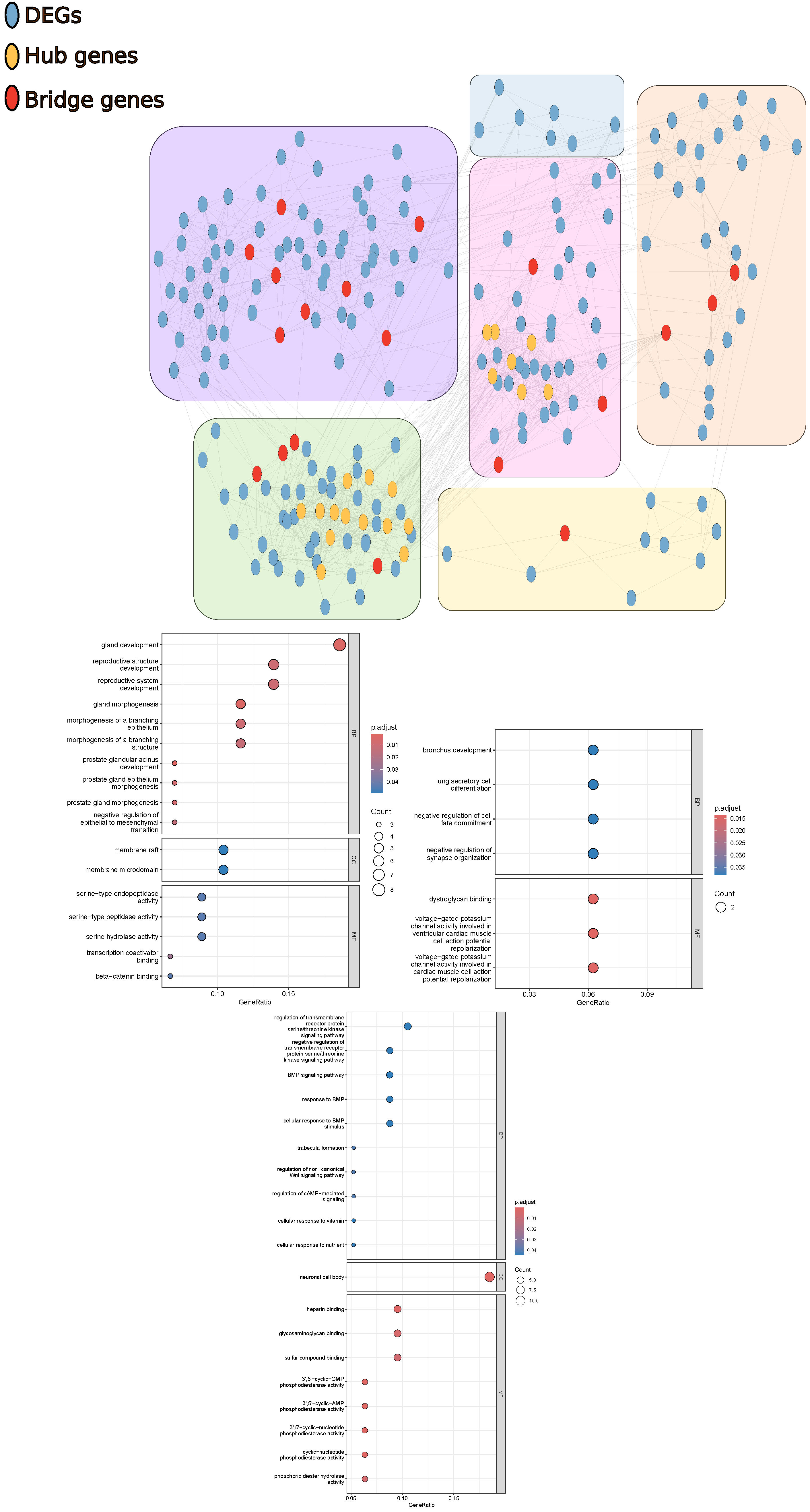
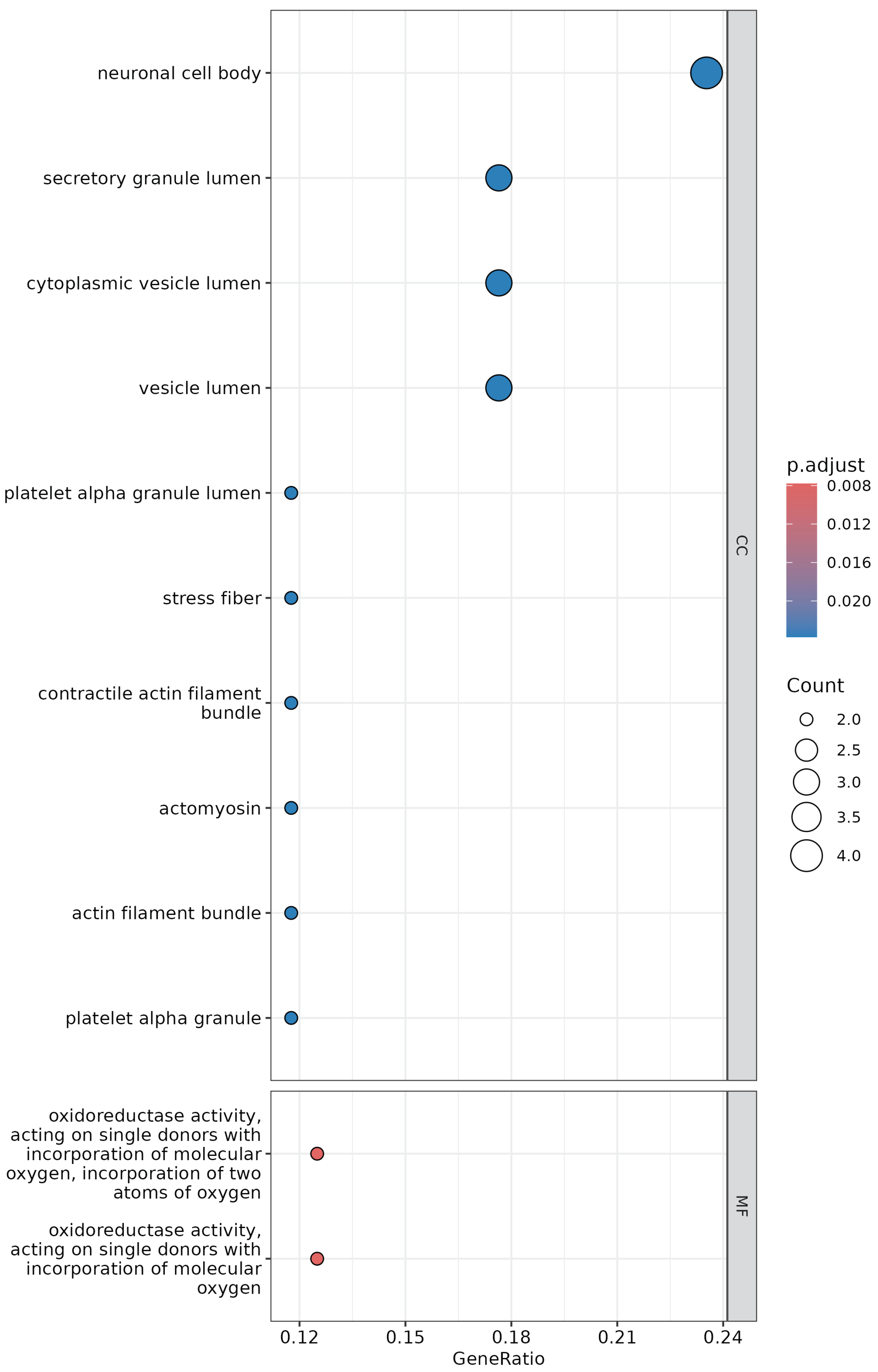
3.5. Gene Co-Expression Network Analysis

Following the selection and refinement of the most appropriate stromal breast tumoral GCN and stromal prostate tumoral GCN, the next step involved conducting a series of analyses to gain insights into the biological mechanisms represented in the networks, with the aim of biomarker discovery. For this purpose, topological and enrichment analyses were performed. Topological analysis involved the identification of hubs and clustering, which was followed by an enrichment analysis of the clusters generated in each co-expression network.

Comparing the final co-expression networks chosen under the 0.75 threshold for both normal and tumor stromal breast samples, we found a total of 16,646 interactions in the normal co-expression network, of which 15,975 were interactions unique to this co-expression network; the tumor co-expression network was made up of 18,595 interactions, of which 17,924 were unique to this co-expression network.

The node degree distributions among the four reconstructed co-expression networks are detailed in Figure A2. Above 20 nodes with higher degree values were considered hubs in each co-expression network. These hubs are shown in

Table A6. The top 20 genes based on co-expression network centrality measures in the stromal breast normal GCN with a 0.75 threshold value without common interactions.

Stromal Breast Normal
Degree Hubs	Score	Betweenness	Score	Closeness	Score	Eigenvector	Score
DOC2B	98.0	AEBP1	5352	ARSA	352.5	DOC2B	0.13
SH2D3C	95.0	GSN	4042.1	SH2D3C	352.3	SH2D3C	0.12
ARSA	94.0	LMO2	3853.0	ADCK2	351.6	ANKRD2-0A11P	0.12
MYH9	94.0	MMP11	3844.5	ANKRD2-0A11P	350.9	MYH9	0.12
ANKRD2-0A11P	91.0	CRTAM	3702.3	RGMA	350.6	ARSA	0.12
RGMA	91.0	SH3BGRL2	3672	SHISA2	350.1	C1orf122	0.12
FAM110D	91.0	ENTREP1	3489.3	C1orf122	350.1	DACT3	0.11
GRP	89.0	NLRC3	3411.1	DOC2B	349.9	SPP1	0.11
ADCK2	88.0	CAVIN2	3403.9	GRP	349.8	RGMA	0.11
C1orf122	88.0	USP36	3377.1	CCDC178	347.9	FAM110D	0.11
LY86	88.0	RGS10	3303.2	SPP1	347.9	GRP	0.11
FDX2	87.0	RSAD2	3251.7	MFAP2	346.8	FDX2	0.11
DACT3	87.0	LEPR	3237.0	EVC	346.7	EVC	0.11
SPP1	87.0	ANLN	3199	LY86	346.5	RAPGEF3	0.11
SHISA2	85.0	JPT1	3168.7	OTULINL	346.4	ITGA7	0.11
RAPGEF3	85.0	TLL2	3159.5	MYH9	346.4	LY86	0.11
EVC	85.0	EXOC6	3146.4	RAPGEF3	346.2	CCN4	0.11
CCN4	85.0	C19orf53	3131.7	DACT3	345.7	OTULINL	0.11
FAM110C	85.0	FICD	3116.9	FAM110C	345.6	ADCK2	0.10
CCM2L	84.0	THBD	3065.2	LOXL2	345.1	FAM241A	0.10

,

Table A7. The top 20 genes based on co-expression network centrality measures in the stromal breast tumor GCN with a 0.75 threshold value without common interactions.

Stromal Breast Cancer
Degree Hubs	Score	Betweenness	Score	Closeness	Score	Eigenvector	Score
LONP2	107.0	HMGN3	7460.8	LONP2	361.1	CRNDE	0.20
ST6GAL2	105.0	LOXL2	6723.3	ST6GAL2	360.4	PRR15L	0.19
SUN1	104.0	CMTM3	4674.1	SUN1	359.9	PDLIM5	0.18
GPR137B	102.0	GLMP	4422.6	GPR137B	358.9	SPON2	0.18
RIPOR3	99.0	MYO5B	4365.5	MAP7D1	357.6	GATA6-AS1	0.18
DYRK2	99.0	PTGS1	4295.2	MCTS1	355.8	LEF1-AS1	0.17
MAP7D1	99.0	NKTR	4222.7	COL5A1	355.0	CDH1	0.17
SNRK	98.0	SEMA3C	4044.4	LGALS1	353.6	APBA2	0.16
SYNDIG1	97.0	CCR5	3963.5	DYRK2	353.5	GPR160	0.16
MATN3	97.0	KIF26B	3924.3	SNRK	352.6	ARFGEF3	0.16
MCTS1	96.0	VOPP1	3832.7	CLK1	352.6	RAB25	0.16
SH3BGRL2	96.0	JPT1	3769.8	INPP1	351.8	HOXB13	0.16
CLK1	95.0	FNDC1	3662.7	SYNDIG1	351.5	HOXC6	0.16
COL5A1	95.0	PCNA	3603.4	MMP13	351.3	EHF	0.16
LGALS1	95.0	SLIT3	3500.1	MATN3	350.9	IER5L	0.15
ALDH1L2	94.0	LINC01614	3395.4	LRRC59	350.8	SPDEF	0.15
DEPDC7	93.0	PIGP	3349.7	ALDH1L2	350.4	FOLH1B	0.15
PROS1	92.0	SPP1	3322.5	PGM1	349.3	DUSP6	0.15
NAP1L5	92.0	NR2F2	3260.2	DEPDC7	349.2	PCDH10-DT	0.14
LRRC59	92.0	LOC1053-77134	3246	HECW2-AS1	348.9	SORD	0.14

,

Table A8. The top 20 genes based on co-expression network centrality measures in the stromal prostate normal GCN with a 0.75 threshold value without common interactions.

Stromal Prostate Normal
Degree Hubs	Score	Betweenness	Score	Closeness	Score	Eigenvector	Score
TIMP4	42.0	PENK	1862.6	TIMP4	101.5	RBP4	0.20
SMTNL2	40.0	STAC	1796.2	SMTNL2	99.9	NAT2	0.20
RBP4	39.0	AGR2	1771.1	RBP4	99.1	TIMP4	0.20
NAT2	38.0	MB	1691.4	CCDC85A	99.1	SMTNL2	0.20
CCDC85A	37.0	PCDH10-DT	1613.0	NAT2	98.2	ARHGA-P28	0.19
KLHL14	36.0	TBX5-AS1	1601.9	ARHGA-P28	97.3	CCDC85A	0.19
IGSF1	35.0	ERG	1517.0	PDE3B	96.8	CFD	0.18
PDE3B	35.0	PEX14	1364.4	MLC1	96.5	IGSF1	0.18
ARHGA-P28	35.0	SPDEF	1349	TRHDE	96.2	LOC10192-7668	0.18
RSPH9	33.0	LINC03026	1334.4	GRTP1-AS1	96.1	PDE3B	0.18
TRHDE	33.0	CLGN	1311.5	IGSF1	96.0	KLHL14	0.18
ODAD3	33.0	FXYD6	1300.3	RNF112	95.7	RSPH9	0.17
CFD	33.0	PPL	1287.9	LY6G6D	94.9	FBXO2	0.17
LOC10192-7668	33.0	PRSS35	1270.1	KLHL14	94.9	ODAD3	0.17
LINC01082	32.0	FAM107A	1257.9	RSPH9	94.8	CHGB	0.17
FBXO2	32.0	ADGRD1	1246.4	FBXL21P	94.6	LINC01082	0.17
GRTP1-AS1	31.0	C9orf24	1239.1	LOC10192-7668	94.3	GATA6-AS1	0.16
GATA6-AS1	31.0	TRHDE	1203.1	CFD	94.2	GRTP1-AS1	0.15
CLGN	31.0	TMSB15A	1150.5	ODAD3	94.1	TRHDE	0.15
MLC1	30.0	LRP1B	1150.4	LINC01082	94.0	CLGN	0.15

and

Table A9. The top 20 genes based on co-expression network centrality measures in the stromal prostate tumor GCN with a 0.75 threshold value without common interactions.

Stromal Prostate Cancer
Degree Hubs	Score	Betweenness	Score	Closeness	Score	Eigenvector	Score
CDH1	30.0	SMIM31	2940.4	EHF	90.5	CRNDE	0.20
ARFGEF3	29.0	NELL2	2244.7	CDH1	90	PRR15L	0.19
PRR15L	29.0	SMOC1	2212.8	ARFGEF3	89.7	PDLIM5	0.18
EHF	28.0	PRKAR2B	2178	HOXB13	88.5	SPON2	0.18
SPON2	28.0	LOC10192-7668	2165.4	PRR15L	87.9	GATA6-AS1	0.18
CRNDE	28.0	PTGS1	2016.1	CRNDE	87.8	LEF1-AS1	0.17
HOXB13	27.0	ST8SIA1	1826.6	LEF1-AS1	87.8	CDH1	0.17
PDLIM5	27.0	ADGRD1	1823.9	SPON2	87.2	APBA2	0.16
CXADR	26.0	LRP1B	1771.2	PDLIM5	87.1	GPR160	0.16
FOXA1	26.0	PRAC1	1676.0	HOXC6	87	ARFGEF3	0.16
GATA6-AS1	26.0	MCF2	1549.7	DUSP6	87	RAB25	0.16
LEF1-AS1	26.0	EHF	1505.7	CXADR	86.8	HOXB13	0.16
HOXC6	26.0	TSLP	1492.5	APBA2	86.6	HOXC6	0.16
GPR160	25.0	CSGALN-ACT1	1487.7	GATA6-AS1	86.6	EHF	0.16
APBA2	25.0	PENK	1467.1	SORD	86.4	IER5L	0.15
SORD	24.0	FRRS1L	1429.8	RBM47	86.1	SPDEF	0.15
RAB25	24.0	RBP4	1419.3	MAP2	85.8	FOLH1B	0.15
DUSP6	24.0	RAB37	1304.7	TRPM8	85.4	DUSP6	0.15
LINC03026	23.0	PLA1A	1300.7	GPR160	85.3	PCDH10-DT	0.14
TRPM8	23.0	FOXF2	1299.4	DKK1	84.9	SORD	0.14

.

Table A6 and Table A7 display the top 20 most connected genes in each of the normal and tumor-specific breast co-expression networks. The average number of interactions among the hub genes selected for the breast normal stromal cell co-expression network was 98, while for the breast cancer stromal cell co-expression network, this was 107 degree. Of the 20 hubs selected for normal and tumor co-expression networks, no common genes were found; therefore, the hubs highlighted are network-specific.

Despite the lack of complete concurrence among the 40 hub genes identified independently in both co-expression network types, a substantial overlap of 36 hub genes existed within the shared interactions.

The majority of hub genes identified in both normal and tumor co-expression networks exhibited elevated values of closeness and eigenvector centrality. This indicates their proximity to all other genes in the co-expression network, facilitating efficient communication and connectivity with other crucial genes.

Comparing the final co-expression networks chosen under the 0.75 threshold for both normal and tumor stromal prostate samples, we found a total of 1678 interactions in the normal network, of which 1619 were interactions unique to this co-expression network; the tumor co-expression network was made up of 1352 interactions, of which 1333 were unique to this co-expression network.

Table A8 and Table A9 display the top 20 most connected genes in each of the normal and tumor-specific networks. The average number of interactions among the hub genes selected for the normal stromal prostate co-expression network was 42, while for the prostate cancer stromal co-expression network, this was 30.

Among the 40 hub genes identified independently in both co-expression network types, half were found as part of the shared interactions between the normal and tumor graphs, and the other half were found without shared interactions in the normal graph and in the tumor graph.

The majority of hub genes identified in both normal and tumor co-expression networks exhibited elevated values of closeness and eigenvector centrality. This indicates their proximity to all other genes in the co-expression network, facilitating efficient communication and connectivity with other crucial genes.

The subsequent step in the topological analysis involved clustering the co-expression networks to identify groups of highly connected genes that may participate in similar biological processes. This method enabled the identification of functional modules and sub-networks, thus simplifying the subsequent enrichment analysis.

Table A5. Clustering analysis summary for breast and prostate Tumor networks.

	Cluster	Avg Nodes	Avg Edges
Breast tumor	3	257.67	5418.33
Prostate tumor	6	36.33	188.83

contains a summary of the clusters obtained for each breast and prostate tumor interaction network.

Two clusters with more than 10 genes were generated for stromal breast tumor (Figure 4), and four clusters with more than 10 genes were generated for the stromal prostate tumor GCN (Figure 5), which had a lower density in comparison. GO enrichment and KEGG analysis were performed on each of the clusters generated, allowing for the identification of functional genetic profiles within the co-expression network. This step enabled a better understanding of the biological mechanisms and pathways associated with the different clusters generated for each GCN.

In the context of the clusters generated within breast stromal cells (Figure 4), two clusters are related due to the interaction of some of their genes, but the metabolic processes in which the genes of each cluster are involved are different. The green cluster contains all the hub genes found in this GCN and is associated with the regulation of cellular differentiation. The other brown cluster is associated with the extracellular matrix, pathways such as focal adhesion, and ECM–receptor interaction. The bridging genes, identified as the top genes with high betweenness centrality values, are distributed in all three clusters of the co-expression network. However, it is noteworthy that the green cluster and brown cluster have the highest presence of these genes.

For green cluster, pink cluster, and purple cluster related to prostate stromal cells, two clusters particularly stand out due to the distribution of hub genes (Figure 5). The green cluster emerged as the most noteworthy, harboring 13 out of the 20 hub genes with GO terms associated with prostate gland morphogenesis, and the pink cluster has seven hub genes and GO terms related to regulation of cell differentiation. Genes facilitating connections between distinct segments of the co-expression network, highlighted in red, were found in five out of the six clusters. Notably, the purple cluster stands out with the highest abundance of these connecting genes. The genes present in this cluster are related to the regulation of different metabolic pathways of cellular proliferation growth factor signaling.

4. Discussion

Tumors develop a unique TME that features different compositions of cancerous, non-cancerous, stromal, and immune cells in each phase of cancer progression. The different cell subtypes of the TME interact with each other but also with components of the ECM surrounding the cells [61]. The TME plays a crucial role in the progression of tumors, influencing key processes such as tumor growth, invasion, and metastasis. Additionally, the TME significantly impacts the immune response against the tumor, either by creating an immunosuppressive environment or by stimulating anti-tumor immune responses [4].

The objective of this study was to compare the stromal responses in breast and prostate cancer. Additionally, the study aimed to propose novel biomarkers related to the tumor microenvironment of both cancer types using an in silico approach following the pipeline illustrated in Figure 1. The following topics can be discussed based on the results obtained.

4.1. Differential Expression Analysis Revealed Significant Differences between Stromal Breast Tumor and Stromal Prostate Tumor

According to the results obtained in the exploratory analysis and the differential expression analysis performed on the expression data, there is a difference in the way the stromal reaction to invasion by breast and prostate tumors may impact tumor progression.

The MDS plot (see Figure 2) reveals substantial variation in the distances between the breast and prostate sample groups, particularly in terms of logFC. The large distances between the samples in the female group and the samples in the male group stand out. Additionally, the distance between normal and tumor samples in the female group is larger than that observed between normal and tumor samples in the prostate group. Furthermore, the differential expression analysis highlighted a significantly higher number of DEGs in stromal tissue surrounding invasive breast tumors (776 DEGs) compared to stromal tissue surrounding invasive prostate tumors (218 DEGs). These findings suggest a major role for stromal cells in the development of breast cancer over that in prostate cancer. This disparity may stem from inherent biological differences between male and female individuals, including sex-specific hormonal, genetic, and physiological factors that contribute to the pathogenesis and progression of breast and prostate cancers.

It is important to note that the heterogeneity within the breast tumor samples was higher in comparison with the prostate tumor samples. In the first case, the majority of the patients exhibited lymph node metastasis, indicating an advanced disease stage [39]. Although both sample groups—breast tumor and prostate tumor samples—were obtained from primary tumor sites, the difference in disease stage could have influenced the number of DEGs identified within both tumor types.

Of the DEGs obtained from breast and prostate samples, most were organ-exclusive. They had only 17 genes in common (see Figure 3). Furthermore, a GO enrichment analysis of the 17 genes revealed common cellular annotations (Figure A1). The majority of these genes, which are shared between stromal cells in prostate and breast cancers, exhibited consistent regulatory patterns. However, there were exceptions, such as TGFB3 (Transforming growth factor beta-3 proprotein), PTGS1 (Prostaglandin G/H synthase 1), DUSP6 (Dual specificity protein phosphatase 6), SASH1 (SAM and SH3 domain-containing protein 1), and FIGN (Fidgetin), which demonstrated distinct regulations depending on the type of tumor (see

Table A2. Common differential genes and their regulation in breast stromal (NB vs. TB) and prostate stromal (NP vs. TP) groups.

Gene ID	Regulation NB vs. TB	Regulation NP vs. TP
KLHL14	downregulated	downregulated
TGFB3	upregulated	downregulated
PDLIM5	upregulated	upregulated
PPL	downregulated	downregulated
PTGS1	upregulated	downregulated
CFD	downregulated	downregulated
ASPA	downregulated	downregulated
FAM107A	downregulated	downregulated
DUSP6	downregulated	upregulated
GPM6A	downregulated	downregulated
BMPR1B	upregulated	upregulated
SASH1	downregulated	upregulated
PENK	downregulated	downregulated
FIGN	downregulated	upregulated
MAL2	upregulated	upregulated
C16orf89	downregulated	downregulated
BCO2	downregulated	downregulated

), which could be linked to the progression of the tumor. These genes have been associated with growth factors, the gene regulation that promotes cell differentiation, cell migration, and microtubule regulation, respectively [62,63,64,65,66]. Nevertheless, these DEGs require further experimental validation in both types of cancer.

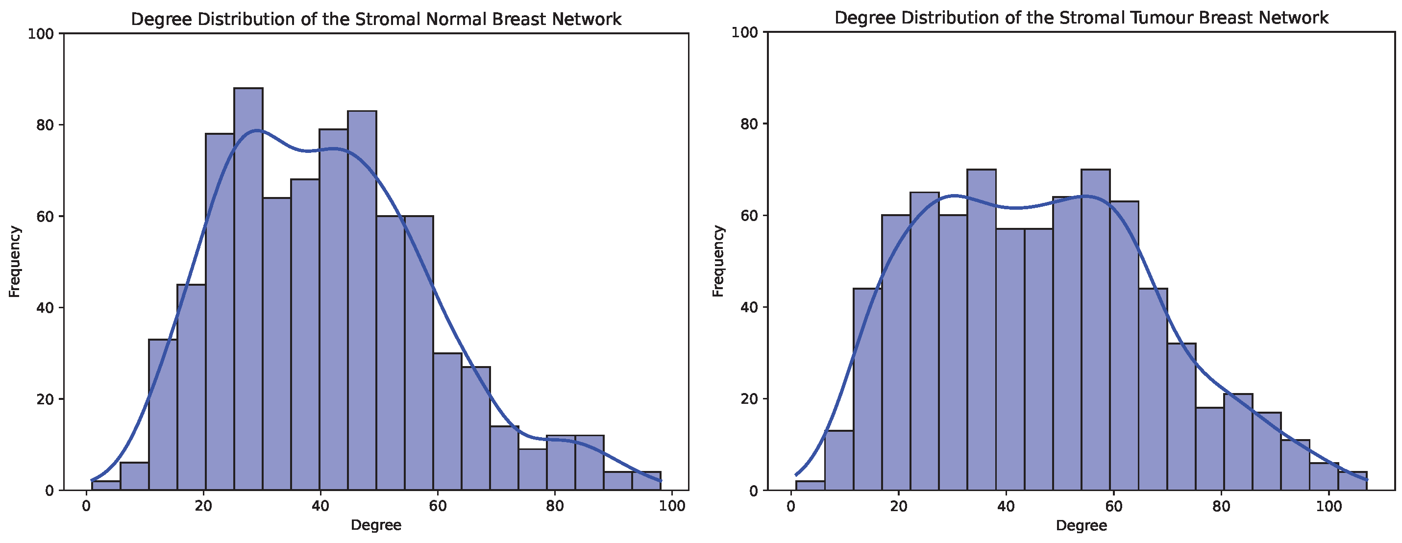
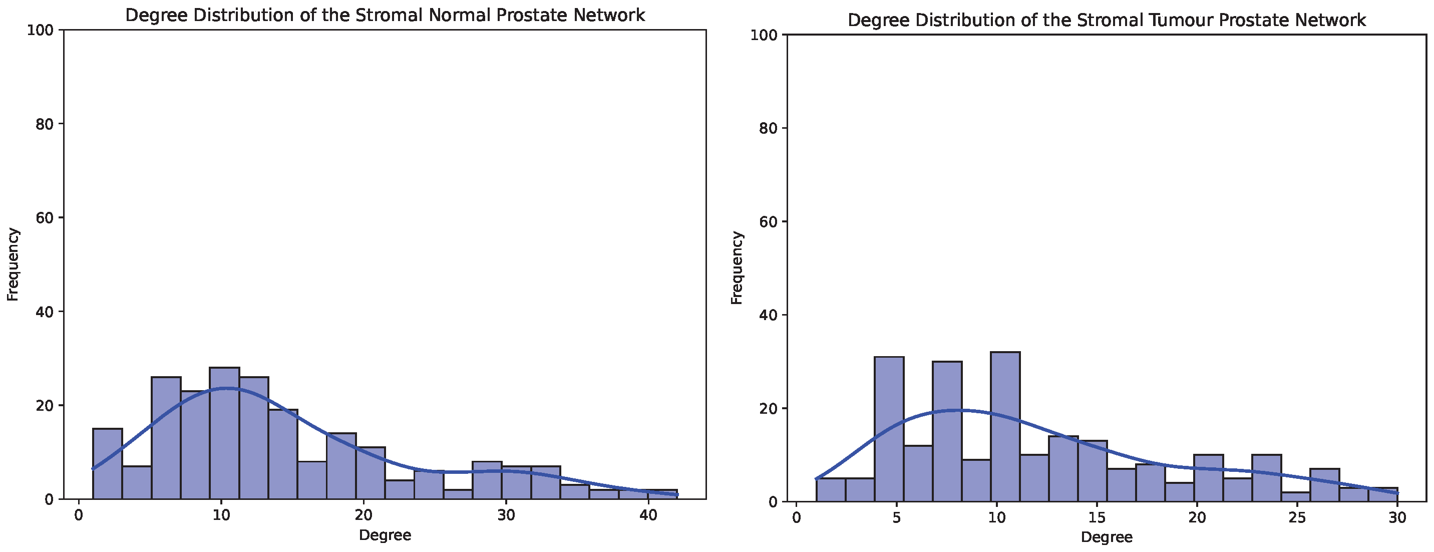
4.2. Exploratory Analysis in Stromal Breast and Prostate Co-Expression Networks

The differences observed in the MSD plots and after differential expression analysis were confirmed after modeling the co-expression networks obtained for each of the case studies: stromal normal breast and prostate and stromal tumor breast and prostate.

A comparative analysis between the normal stromal and stromal breast tumor co-expression networks shed light on those hub genes present in both co-expression networks but that did not share interactions. This discovery implies that the four genes excluded from shared interactions may exert a critical role in distinct contexts, contingent on their expression levels. Specifically, the SPP1 (Osteopontin) and ARSA (Arylsulfatase A) genes were discerned in the normal stromal breast network, while RIPOR3 (RIPOR family member 3) and LGALS1 (Galectin-1) were identified in the tumor stromal breast network.

Specifically, in the case of the hub genes present in the tumor breast (Table A7), 65% of them have previously been found to be biomarkers in breast cancer studies. SUN1 (SUN domain-containing protein 1) serves as a constituent of the Linker of Nucleoskeleton and Cytoskeleton complex, participating in the linkage between the nuclear lamina and the cytoskeleton [67]. In a study conducted by Matsumoto et al., upregulation of this component was observed in human breast cancer tissues. The authors proposed that the expression of SUN1, along with other cytoskeleton complex genes, may play pivotal pathological roles in the progression of breast cancer [68]. The LGALS1 gene was suggested as a biomarker by Jung et al. [69] in human breast carcinoma tissues, where an elevated expression of Galectin 1 was observed in all cancerous stromal tissues associated with breast cancer. The MAP7D1 (MAP7 domain-containing protein 1) gene was previously proposed as a biomarker by Wu et al. [70] in breast cancer.

Out of the 20 hub genes obtained from both the normal and tumor prostate networks, only the GATA6-AS1 gene is shared; the remaining hub genes are specific to each co-expression network. It is noteworthy that the hub genes derived from the normal network exhibited downregulation, with the exception of GATA6-AS1. In contrast, the hub genes identified in the tumor network displayed overexpression, except for GATA6-AS1 and APBA2 (Amyloid-beta A4 precursor protein-binding family A member 2).

Specifically, in the case of the hub genes present in the tumor prostate co-expression network (Table A9), 60% of them were previously found to be biomarkers in prostate cancer studies. HOXC6 (Homeobox protein Hox-C6), which was reported as a biomarker in another prostate cancer study [71], and GPR160, a G protein-coupled receptor, were overexpressed in prostate cancers, and their effect does not require the involvement of androgen receptors. There inhibition induces apoptosis in prostate cancer cells and therefore has significant effects on cancer cell proliferation and survival [72].

4.3. Gene Expression of Stromal Cells in Breast Tumors Is Related to Focal Adhesion Modifications, While That of Stromal Cells in Prostate Tumors Is Related to Organ Formation and Cell Differentiation

In the context of breast stromal cells, the central genes of the co-expression network were identified as part of one of the three clusters comprising the final co-expression network, as summarized in Figure 4. The green cluster was associated with the regulation of proteins present in the extracellular matrix, where stromal cells were embedded. Based on the ontogenetic study of the two main clusters obtained, it is suggested that the affected components are those directly involved in extracellular adhesion, possibly in response to a regulatory process facilitated by a collaborative interaction between stromal and tumor cells [73]. Some genes present in the co-expression network contribute to microenvironment remodeling, including HPSE (Heparanase), which enhances cell adhesion to the extracellular matrix independently of its enzymatic activity. This induces Akt1/PKB phosphorylation through lipid rafts, consequently increasing cell motility and invasion [74,75]. Another gene, RHOU (Rho-related GTP-binding protein RhoU) plays a role in the regulation of cell morphology and cytoskeletal organization [76].

In the case of the prostate stromal cells, hub genes of the co-expression network were found to form part of two of the six clusters of which the final co-expression network was composed, a summary of the co-expression network annotation is given in Figure 5. In contrast to breast cancer stromal cells, there were fewer differential genes expression difference between the normal and tumor prostate stromal tissue. This suggests that breast cancer stromal cells have a much greater role in tumor cell development than prostate stromal cells. The hub genes found within the main prostate network were distributed between the green cluster and pink cluster. Both clusters were related to organ maintenance, epithelial tissue differentiation, and morphology. A distinctive pattern is observed that reveals a close relationship with cell morphology and the process of mesenchymal development. Those present in both clusters appear to be intrinsically linked to the regulation of cell shape and structure, being themselves responsible for the stromal abnormality in prostate cancers rather than being mediated in response to the environment, as in the case of breast cancer. Some of the genes involved in this process are S100A4, a calcium-binding protein that plays a role in various cellular processes, including motility, angiogenesis, cell differentiation, apoptosis, and autophagy [77]; and HPN, which plays a role in cell growth and maintenance of cell morphology [78]. These findings highlight the importance of stromal cell differentiation in the plasticity of prostate tumors. This modulation of stromal cell morphology is observed in histological sections. Some of the patterns include hypercellular stroma with scattered atypical but degenerative atypical cells mixed with benign prostatic glands, and hypercellular strychoma consisting of soft spindle-shaped stromal cells mixed with benign glands, and they may also contain atypical and degenerative stromal cells that may be associated with a variety of benign epithelial proliferations, including basal cell hyperplasia, adenosis, and sclerosing adenosis [79,80].

In summary, our network-generation method was able to generate the study co-expression networks from differentially expressed genes of stromal cells in the context of both breast and prostate cancer and find patterns of differences in the mode of stromal cell development relative to each case in particular.

4.4. ST6GAL2, RIPOR3, COL5A1, and DEPDC7 Are Potential Biomarkers in the Breast Tumor Microenvironment

As mentioned earlier, a comprehensive literature review was conducted to investigate the association of the identified hub genes with stromal cells in breast cancer. From the study of the GCN, we can highlight the hub genes ST6GAL2, RIPOR3, COL5A1, and DEPDC7 as possible biomarkers in the context of stromal cells in breast tumors, as they have been characterized in other cancer cases.

There is no specific literature about ST6GAL2 (Beta-galactoside alpha-2,6-sialyltransferase 2) with breast cancer evidence, but this gene has been highlighted in follicular thyroid carcinoma [81].

While there is limited specific literature evidence about the role of the RIPOR3 gene in breast cancer, it has been studied in other cancer types. Notably, RIPOR3 has shown a disregulation at oral squamus cell carcinoma of the mobile tongue [82]. At present, reports in the literature on the RIPOR3 gene are limited.

Another possible biomarker is COL5A1 (Collagen alpha-1(V) chain), and though there is no specific literature about this gene associated with breast tumor, it was associated with the progression of gastric cancer in humans [83].

Finally, DEPDC7 (DEP domain-containing protein 7) is proposed as a biomarker, but its function is poorly understood. Liao et al. investigated the disregulation of this gene in two hepatoma cell lines, as well as the cell proliferation, cell cycle progression, cell migration, and invasion of these cells, suggesting that DEPDC7 is a tumor suppress gene [84].

4.5. GATA6-AS1, ARFGEF3, PRR15L, and APBA2 Are Potential Biomarkers in the Prostate Tumor Microenvironment

A comprehensive literature review was conducted to investigate the association of the identified hub genes with stromal cells in prostate cancer. From the study of the GCN, we can highlight the hub genes GATA6-AS1, ARFGEF3, PRR15L, APBA2, and LINC03026 as possible biomarkers in the context of stromal cells in prostate tumors, as they have been characterized in other cancer cases.

The GATA6-AS1 lncRNA has been linked to the expression of F-box proteins [85], which play an important role in the degradation of key proteins in cellular regulation and tumorigenesis [86]. It has been studied in the context of lung, gastric, and ovarian cancer in association with the inhibition of signaling pathways and prevention of epithelial–mesenchymal transition [87,88]. The hub gene GATA6-AS1 was in the green cluster and had 26 interactions. Of these interactions, fifteen were hub genes. It should be noted that GATA6-AS1 is also one of the hub genes found in the results obtained for normal stromal breast and stands out in this dataset as the only one of the calculated hub genes that showed upregulation with respect to the rest. The genes with which they were related within the co-expression network were found both in the green cluter and pink cluster, so they participated in the regulation of both clusters. This gene interacts with the gene HOXC6, which was present in the pink cluster, which was previously reported as a biomarker in another prostate cancer study [71].

ARFGEF3 or BIG3 (Brefeldin A-inhibited guanine nucleotide-exchange protein 3). Kim et al. identified BIG3 as significantly overexpressed in the great majority of breast cancer cases and breast cancer cell lines [89].

The bibliographical information regarding PRR15L (Proline-rich protein 15-like protein) gene is scarce. We can highlight the study in Mizuguchi et al. [90], where PRR15L-RSPO2 fusion was identified, which expands the variations of RSPO fusions in colorectal neoplasms. This gene was present in the green cluster and interacted with 29 genes, some of which are closely related to studies on prostate cancer, for example, DKK1 (Dickkopf-related protein 1), whose protein negatively regulates the Wnt/$\beta$-catenin signalling pathway, with therapeutics targeting of it in clinical trials for cancer patients [91].

Finally, APBA2 (Amyloid-beta A4 precursor protein-binding family A member 2) was proposed as an epigenetic regulatory gene involved in multiple cancer-related pathways in breast cancer [92]. This gene was present in the pink cluster and interacted with another characterized gene like FOXQ1 (Forkhead box protein Q1), which is a transcription factor that has been studied in several types of cancer, has been found to be upregulated or downregulated in different types of cancer, and has therefore already been suggested as a prognostic biomarker for several types of tumors [93].

5. Conclusions

In this work, we presented a computational study of GCNs to identify breast and prostate cancer biomarkers. To do so, we also introduced an ensemble method for the inference of GCNs. The method is based on three different correlation algorithms (Pearson, Kendall, and Spearman). Thus, only if two or more coefficients determine that the relationship is significant will it be established as valid. As a result, the final co-expression network obtained offered a higher level of reliability than if only a single coefficient had been used.

On the other hand, the main results of the study revealed different behaviors depending on the organ in which the cancer develops. It was found that breast cancer stromal cells are related to the maintenance of the extracellular matrix through modifications in the focal-adhesion that are part of the stromal tissue. On the other hand, prostate cancer stromal cells are related to cell differentiation, leading to abnormal development of stromal cells. Finally, potential biomarkers were suggested; in the case of breast tumor, ST6GAL2, RIPOR3, COL5A1, and DEPDC7 were found, and in the case of prostate tumor, the genes were GATA6-AS1, ARFGEF3, PRR15L, and APBA2. These results demonstrate the usefulness of the method in the field of biomarker discovery.

As future work, we are currently working on two main points in the context of this work: delving deeper into the study of prostate and breast cancer, and in another sense, improving the co-expression network inference method to achieve better results. To obtain a better understanding of these cancers, we are using additional datasets, such as RNA-Seqs and even single-cell, to verify the results obtained in the present study. On the other hand, we are also working to improve the inference algorithm from two points of view: (a) using other algorithms or correlation coefficients in the ensemble co-expression network generation step to enhance the results, and (b) allowing multi-input of data to improve the reliability of the conclusions obtained.

References

1. Arnold, M.; Morgan, E.; Rumgay, H.; Mafra, A.; Singh, D.; Laversanne, M.; Vignat, J.; Gralow, J.R.; Cardoso, F.; Siesling, S.; et al. Current and future burden of breast cancer: Global statistics for 2020 and 2040. Breast 2022, 66, 15–23. [Google Scholar] [CrossRef] [PubMed]
2. Withrow, D.; Pilleron, S.; Nikita, N.; Ferlay, J.; Sharma, S.; Nicholson, B.; Rebbeck, T.R.; Lu-Yao, G. Current and projected number of years of life lost due to prostate cancer: A global study. Prostate 2022, 82, 1088–1097. [Google Scholar] [CrossRef] [PubMed]
3. Alekseenko, I.V.; Chernov, I.P.; Kostrov, S.V.; Sverdlov, E.D. Are synapse-like structures a possible way for crosstalk of cancer with its microenvironment? Cancers 2020, 12, 806. [Google Scholar] [CrossRef] [PubMed]
4. Sund, M.; Kalluri, R. Tumor stroma derived biomarkers in cancer. Cancer Metastasis Rev. 2009, 28, 177–183. [Google Scholar] [CrossRef] [PubMed]
5. Mao, Y.; Keller, E.T.; Garfield, D.H.; Shen, K.; Wang, J. Stromal cells in tumor microenvironment and breast cancer. Cancer Metastasis Rev. 2013, 32, 303–315. [Google Scholar] [CrossRef]
6. Kawada, M.; Inoue, H.; Usami, I.; Ikeda, D. Phthoxazolin A inhibits prostate cancer growth by modulating tumor–stromal cell interactions. Cancer Sci. 2009, 100, 150–157. [Google Scholar] [CrossRef] [PubMed]
7. Hong, M.; Tao, S.; Zhang, L.; Diao, L.T.; Huang, X.; Huang, S.; Xie, S.J.; Xiao, Z.D.; Zhang, H. RNA sequencing: New technologies and applications in cancer research. J. Hematol. Oncol. 2020, 13, 166. [Google Scholar] [CrossRef] [PubMed]
8. Riquelme Medina, I.; Lubovac-Pilav, Z. Gene co-expression network analysis for identifying modules and functionally enriched pathways in type 1 diabetes. PLoS ONE 2016, 11, e0156006. [Google Scholar] [CrossRef]
9. Redekar, S.S.; Varma, S.L.; Bhattacharjee, A. Gene co-expression network construction and analysis for identification of genetic biomarkers associated with glioblastoma multiforme using topological findings. J. Egypt. Natl. Cancer Inst. 2023, 35, 22. [Google Scholar] [CrossRef]
10. Jiang, Y.H.; Long, J.; Zhao, Z.B.; Li, L.; Lian, Z.X.; Liang, Z.; Wu, J.R. Gene co-expression network based on part mutual information for gene-to-gene relationship and gene-cancer correlation analysis. BMC Bioinform. 2022, 23, 194. [Google Scholar] [CrossRef]
11. Huang, R.; He, Y.; Sun, B.; Liu, B. Bioinformatic Analysis Identifies Three Potentially Key Differentially Expressed Genes in Peripheral Blood Mononuclear Cells of Patients with Takayasu’s Arteritis. Cell J. 2018, 19, 647–653. [Google Scholar] [CrossRef]
12. Brugere, I.; Gallagher, B.; Berger-Wolf, T.Y. Network structure inference, a survey: Motivations, methods, and applications. ACM Comput. Surv. (CSUR) 2018, 51, 24. [Google Scholar] [CrossRef]
13. Langfelder, P.; Horvath, S. WGCNA: An R package for weighted correlation network analysis. BMC Bioinform. 2008, 9, 559. [Google Scholar] [CrossRef] [PubMed]
14. Hsu, H.M.; Chu, C.M.; Chang, Y.J.; Yu, J.C.; Chen, C.T.; Jian, C.E.; Lee, C.Y.; Chiang, Y.T.; Chang, C.W.; Chang, Y.T. Six novel immunoglobulin genes as biomarkers for better prognosis in triple-negative breast cancer by gene co-expression network analysis. Sci. Rep. 2019, 9, 4484. [Google Scholar] [CrossRef]
15. Wang, L.; Liao, Z. Mixture prior for sparse signals with dependent covariance structure. PLoS ONE 2023, 18, e0284284. [Google Scholar] [CrossRef]
16. van den Heuvel, E.; Zhan, Z. Myths about linear and monotonic associations: Pearson’sr, Spearman’s ρ, and Kendall’s τ. Am. Stat. 2022, 76, 44–52. [Google Scholar] [CrossRef]
17. Delgado-Chaves, F.M.; Gómez-Vela, F.; García-Torres, M.; Divina, F.; Vazquez Noguera, J.L. Computational inference of gene co-expression networks for the identification of lung carcinoma biomarkers: An ensemble approach. Genes 2019, 10, 962. [Google Scholar] [CrossRef] [PubMed]
18. Ovens, K.; Eames, B.F.; McQuillan, I. Comparative analyses of gene co-expression networks: Implementations and applications in the study of evolution. Front. Genet. 2021, 12, 695399. [Google Scholar] [CrossRef]
19. Tang, J.; Kong, D.; Cui, Q.; Wang, K.; Zhang, D.; Gong, Y.; Wu, G. Prognostic genes of breast cancer identified by gene co-expression network analysis. Front. Oncol. 2018, 8, 374. [Google Scholar] [CrossRef]
20. Zhou, Q.; Ren, J.; Hou, J.; Wang, G.; Ju, L.; Xiao, Y.; Gong, Y. Co-expression network analysis identified candidate biomarkers in association with progression and prognosis of breast cancer. J. Cancer Res. Clin. Oncol. 2019, 145, 2383–2396. [Google Scholar] [CrossRef]
21. Adhami, M.; MotieGhader, H.; Haghdoost, A.A.; Afshar, R.M.; Sadeghi, B. Gene co-expression network approach for predicting prognostic microRNA biomarkers in different subtypes of breast cancer. Genomics 2020, 112, 135–143. [Google Scholar] [CrossRef] [PubMed]
22. Ye, Z. Identification of T cell-related biomarkers for breast cancer based on weighted gene co-expression network analysis. J. Chemother. 2023, 35, 298–306. [Google Scholar] [CrossRef] [PubMed]
23. Song, Z.-Y.; Chao, F.; Zhuo, Z.; Ma, Z.; Li, W.; Chen, G. Identification of hub genes in prostate cancer using robust rank aggregation and weighted gene co-expression network analysis. Aging 2019, 11, 4736. [Google Scholar] [CrossRef] [PubMed]
24. Xu, N.; Dong, R.N.; Lin, T.T.; Lin, T.; Lin, Y.Z.; Chen, S.H.; Zhu, J.M.; Ke, Z.B.; Huang, F.; Chen, Y.H.; et al. Development and validation of novel biomarkers related to M2 macrophages infiltration by weighted gene co-expression network analysis in prostate cancer. Front. Oncol. 2021, 11, 634075. [Google Scholar] [CrossRef] [PubMed]
25. Liu, M.; Chen, M.Y.; Huang, J.M.; Liu, Q.; Wang, L.; Liu, R.; Yang, N.; Huang, W.H.; Zhang, W. LncRNA weighted gene co-expression network analysis reveals novel biomarkers related to prostate cancer metastasis. BMC Med. Genom. 2022, 15, 256. [Google Scholar] [CrossRef]
26. Deng, J.L.; Xu, Y.-H.; Wang, G. Identification of potential crucial genes and key pathways in breast cancer using bioinformatic analysis. Front. Genet. 2019, 10, 695. [Google Scholar] [CrossRef]
27. Zhu, L.; Ding, Y.; Chen, C.Y.; Wang, L.; Huo, Z.; Kim, S.; Sotiriou, C.; Oesterreich, S.; Tseng, G.C. MetaDCN: Meta-analysis framework for differential co-expression network detection with an application in breast cancer. Bioinformatics 2017, 33, 1121–1129. [Google Scholar] [CrossRef]
28. Margolin, A.A.; Nemenman, I.; Basso, K.; Wiggins, C.; Stolovitzky, G.; Favera, R.D.; Califano, A. ARACNE: An algorithm for the reconstruction of gene regulatory networks in a mammalian cellular context. BMC Bioinform. 2006, 7, S7. [Google Scholar] [CrossRef] [PubMed]
29. Hawley, J.E.; Obradovic, A.Z.; Dallos, M.C.; Lim, E.A.; Runcie, K.; Ager, C.R.; McKiernan, J.; Anderson, C.B.; Decastro, J.; Weintraub, J.; et al. Single-Cell RNAseq Analysis Reveals Robust, Anti-PD-1-Mediated Increase in Immune Infiltrate in Metastatic Castration-Sensitive Prostate Cancer. bioRxiv 2022, 490968. [Google Scholar] [CrossRef]
30. Decker, A.M.; Decker, J.T.; Jung, Y.; Cackowski, F.C.; Daignault-Newton, S.; Morgan, T.M.; Shea, L.D.; Taichman, R.S. Adrenergic blockade promotes maintenance of dormancy in prostate cancer through upregulation of GAS6. Transl. Oncol. 2020, 13, 100781. [Google Scholar] [CrossRef]
31. Mevik, B.H.; Wehrens, R. The pls Package: Principal Component and Partial Least Squares Regression in R. J. Stat. Softw. 2007, 18, 1–23. [Google Scholar] [CrossRef]
32. Siletz, A.; Schnabel, M.; Kniazeva, E.; Schumacher, A.J.; Shin, S.; Jeruss, J.S.; Shea, L.D. Dynamic transcription factor networks in epithelial-mesenchymal transition in breast cancer models. PLoS ONE 2013, 8, e57180. [Google Scholar] [CrossRef]
33. Haury, A.C.; Mordelet, F.; Vera-Licona, P.; Vert, J.P. TIGRESS: Trustful inference of gene regulation using stability selection. BMC Syst. Biol. 2012, 6, 145. [Google Scholar] [CrossRef] [PubMed]
34. Cutler, A.; Cutler, D.R.; Stevens, J.R. Random forests. In Ensemble Machine Learning: Methods and Applications; Springer: Berlin/Heidelberg, Germany, 2012; pp. 157–175. [Google Scholar] [CrossRef]
35. Faith, J.J.; Hayete, B.; Thaden, J.T.; Mogno, I.; Wierzbowski, J.; Cottarel, G.; Kasif, S.; Collins, J.J.; Gardner, T.S. Large-scale mapping and validation of Escherichia coli transcriptional regulation from a compendium of expression profiles. PLoS Biol. 2007, 5, e8. [Google Scholar] [CrossRef]
36. Meyer, P.E.; Kontos, K.; Lafitte, F.; Bontempi, G. Information-theoretic inference of large transcriptional regulatory networks. EURASIP J. Bioinform. Syst. Biol. 2007, 2007, 1–9. [Google Scholar] [CrossRef] [PubMed]
37. Ferraz, R.S.; Cavalcante, J.V.F.; Magalhães, L.; Ribeiro-dos Santos, Â.; Dalmolin, R.J.S. Revealing metastatic castration-resistant prostate cancer master regulator through lncRNAs-centered regulatory network. Cancer Med. 2023, 12, 19279–19290. [Google Scholar] [CrossRef] [PubMed]
38. Gómez-Vela, F.; Delgado-Chaves, F.M.; Rodríguez-Baena, D.S.; García-Torres, M.; Divina, F. Ensemble and Greedy Approach for the Reconstruction of Large Gene Co-Expression Networks. Entropy 2019, 21, 1139. [Google Scholar] [CrossRef]
39. Planche, A.; Bacac, M.; Provero, P.; Fusco, C.; Delorenzi, M.; Stehle, J.C.; Stamenkovic, I. Identification of Prognostic Molecular Features in the Reactive Stroma of Human Breast and Prostate Cancer. PLoS ONE 2011, 6, e18640. [Google Scholar] [CrossRef] [PubMed]
40. Ritchie, M.E.; Phipson, B.; Wu, D.; Hu, Y.; Law, C.W.; Shi, W.; Smyth, G.K. limma powers differential expression analyses for RNA-sequencing and microarray studies. Nucleic Acids Res. 2015, 43, e47. [Google Scholar] [CrossRef]
41. Law, C.W.; Alhamdoosh, M.; Su, S.; Smyth, G.K.; Ritchie, M.E. RNA-seq analysis is easy as 1-2-3 with limma, Glimma and edgeR. F1000Research 2016, 5, 1408. [Google Scholar] [CrossRef]
42. Smyth, G.K. Linear models and empirical bayes methods for assessing differential expression in microarray experiments. Stat. Appl. Genet. Mol. Biol. 2004, 3. [Google Scholar] [CrossRef] [PubMed]
43. Kumari, S.; Nie, J.; Chen, H.; Ma, H.; Stewart, R.; Li, X.; Lu, M.; Taylor, W.; Wei, H. Evaluation of Gene Association Methods for Coexpression Network Construction and Biological Knowledge Discovery. PLoS ONE 2012, 7, e50411. [Google Scholar] [CrossRef] [PubMed]
44. de Siqueira Santos, S.; Takahashi, D.Y.; Nakata, A.; Fujita, A. A Comparative Study of Statistical Methods Used to Identify Dependencies Between Gene Expression Signals. Brief. Bioinform. 2014, 15, 906–918. [Google Scholar] [CrossRef] [PubMed]
45. Virtanen, P.; Gommers, R.; Oliphant, T.E.; Haberland, M.; Reddy, T.; Cournapeau, D.; Burovski, E.; Peterson, P.; Weckesser, W.; Bright, J.; et al. SciPy 1.0: Fundamental algorithms for scientific computing in Python. Nat. Methods 2020, 17, 261–272. [Google Scholar] [CrossRef]
46. Díaz-Montaña, J.J.; Gómez-Vela, F.; Díaz-Díaz, N. GNC–app: A new Cytoscape app to rate gene networks biological coherence using gene–gene indirect relationships. Biosystems 2018, 166, 61–65. [Google Scholar] [CrossRef] [PubMed]
47. Oughtred, R.; Rust, J.; Chang, C.; Breitkreutz, B.; Stark, C.; Willems, A.; Boucher, L.; Leung, G.; Kolas, N.; Zhang, F.; et al. The BioGRID database: A comprehensive biomedical resource of curated protein, genetic, and chemical interactions. Protein Sci. 2021, 30, 187–200. [Google Scholar] [CrossRef] [PubMed]
48. Gómez-Vela, F.; Lagares, J.A.; Díaz-Díaz, N. Gene network coherence based on prior knowledge using direct and indirect relationships. Comput. Biol. Chem. 2015, 56, 142–151. [Google Scholar] [CrossRef] [PubMed]
49. Gaiteri, C.; Ding, Y.; French, B.; Tseng, G.; Sibille, E. Beyond modules and hubs: The potential of gene coexpression networks for investigating molecular mechanisms of complex brain disorders. Genes Brain Behav. 2014, 13, 13–24. [Google Scholar] [CrossRef] [PubMed]
50. Chin, C.H.; Chen, S.H.; Wu, H.H.; Ho, C.W.; Ko, M.T.; Lin, C.Y. cytoHubba: Identifying hub objects and sub-networks from complex interactome. BMC Syst. Biol. 2014, 8, S11. [Google Scholar] [CrossRef]
51. Su, G.; Kuchinsky, A.; Morris, J.H.; States, D.J.; Meng, F. GLay: Community structure analysis of biological networks. Bioinformatics 2010, 26, 3135–3137. [Google Scholar] [CrossRef]
52. Morris, J.H.; Apeltsin, L.; Newman, A.M.; Baumbach, J.; Wittkop, T.; Su, G.; Bader, G.D.; Ferrin, T.E. clusterMaker: A multi-algorithm clustering plugin for Cytoscape. BMC Bioinform. 2011, 12, 436. [Google Scholar] [CrossRef] [PubMed]
53. Ashburner, M.; Ball, C.A.; Blake, J.A.; Botstein, D.; Butler, H.; Cherry, J.M.; Davis, A.P.; Dolinski, K.; Dwight, S.S.; Eppig, J.T.; et al. Gene ontology: Tool for the unification of biology. Nat. Genet. 2000, 25, 25–29. [Google Scholar] [CrossRef] [PubMed]
54. Tipney, H.; Hunter, L. An introduction to effective use of enrichment analysis software. Hum. Genom. 2010, 4, 202. [Google Scholar] [CrossRef] [PubMed]
55. Kanehisa, M.; Goto, S. KEGG: Kyoto encyclopedia of genes and genomes. Nucleic Acids Res. 2000, 28, 27–30. [Google Scholar] [CrossRef] [PubMed]
56. Yu, G.; Wang, L.G.; Han, Y.; He, Q.Y. clusterProfiler: An R package for comparing biological themes among gene clusters. Omics J. Integr. Biol. 2012, 16, 284–287. [Google Scholar] [CrossRef] [PubMed]
57. Pei, G.; Chen, L.; Zhang, W. WGCNA application to proteomic and metabolomic data analysis. In Methods in Enzymology; Elsevier: Amsterdam, The Netherlands, 2017; Volume 585, pp. 135–158. [Google Scholar]
58. Liu, W.; Li, L.; Ye, H.; Tu, W. Weighted gene co-expression network analysis in biomedicine research. Chin. J. Biotechnol. 2017, 33, 1791–1801. [Google Scholar]
59. Delgado-Chaves, F.M.; Gómez-Vela, F.; Divina, F.; García-Torres, M.; Rodriguez-Baena, D.S. Computational analysis of the global effects of Ly6E in the immune response to coronavirus infection using gene networks. Genes 2020, 11, 831. [Google Scholar] [CrossRef] [PubMed]
60. Saz-Navarro, D.M.; López-Fernández, A.; Gómez-Vela, F.A.; Rodriguez-Baena, D.S. CyEnGNet—App: A new Cytoscape app for the reconstruction of large co-expression networks using an ensemble approach. SoftwareX 2024, 25, 101634. [Google Scholar] [CrossRef]
61. Yu, Y.R.; Ho, P.C. Sculpting tumor microenvironment with immune system: From immunometabolism to immunoediting. Clin. Exp. Immunol. 2019, 197, 153–160. [Google Scholar] [CrossRef]
62. Mukherjee, S.; Diaz Valencia, J.D.; Stewman, S.; Metz, J.; Monnier, S.; Rath, U.; Asenjo, A.B.; Charafeddine, R.A.; Sosa, H.J.; Ross, J.L.; et al. Human Fidgetin is a microtubule severing enzyme and minus-end depolymerase that regulates mitosis. Cell Cycle 2012, 11, 2359–2366. [Google Scholar] [CrossRef]
63. Dauphinee, S.M.; Clayton, A.; Hussainkhel, A.; Yang, C.; Park, Y.J.; Fuller, M.E.; Blonder, J.; Veenstra, T.D.; Karsan, A. SASH1 is a scaffold molecule in endothelial TLR4 signaling. J. Immunol. 2013, 191, 892–901. [Google Scholar] [CrossRef] [PubMed]
64. Sostres, C.; Gargallo, C.J.; Lanas, A. Aspirin, cyclooxygenase inhibition and colorectal cancer. World J. Gastrointest. Pharmacol. Ther. 2014, 5, 40–49. [Google Scholar] [CrossRef] [PubMed]
65. Mishra, A.; Oulès, B.; Pisco, A.O.; Ly, T.; Liakath-Ali, K.; Walko, G.; Viswanathan, P.; Tihy, M.; Nijjher, J.; Dunn, S.J.; et al. A protein phosphatase network controls the temporal and spatial dynamics of differentiation commitment in human epidermis. eLife 2017, 6, e27356. [Google Scholar] [CrossRef] [PubMed]
66. Zhao, B.; Xu, S.; Dong, X.; Lu, C.; Springer, T.A. Prodomain-growth factor swapping in the structure of pro-TGF-β1. J. Biol. Chem. 2018, 293, 1579–1589. [Google Scholar] [CrossRef] [PubMed]
67. Stewart-Hutchinson, P.J.; Hale, C.M.; Wirtz, D.; Hodzic, D. Structural requirements for the assembly of LINC complexes and their function in cellular mechanical stiffness. Exp. Cell Res. 2008, 314, 1892–1905. [Google Scholar] [CrossRef] [PubMed]
68. Matsumoto, A.; Hieda, M.; Yokoyama, Y.; Nishioka, Y.; Yoshidome, K.; Tsujimoto, M.; Matsuura, N. Pérdida global de un componente de lámina nuclear, lamina A/C y componentes complejos LINC SUN1, SUN2 y nesprin-2 en el cáncer de mama. Cancer Med. 2015, 4, 1547–1557. [Google Scholar] [CrossRef] [PubMed]
69. Jung, E.J.; Moon, H.G.; Cho, B.I.; Jeong, C.Y.; Joo, Y.T.; Lee, Y.J.; Hong, S.C.; Choi, S.K.; Ha, W.S.; Kim, J.W.; et al. Galectin-1 expression in cancer-associated stromal cells correlates tumor invasiveness and tumor progression in breast cancer. Int. J. Cancer 2007, 120, 2331–2338. [Google Scholar] [CrossRef] [PubMed]
70. Wu, S.L.; Zhang, X.; Chang, M.; Huang, C.; Qian, J.; Li, Q.; Yuan, F.; Sun, L.; Yu, X.; Cui, X.; et al. Genome-wide 5-Hydroxymethylcytosine Profiling Analysis Identifies MAP7D1 as A Novel Regulator of Lymph Node Metastasis in Breast Cancer. Genom. Proteom. Bioinform. 2021, 19, 64–79. [Google Scholar] [CrossRef]
71. Borziak, K.; Finkelstein, J. Gene Expression Markers of Prognostic Importance for Prostate Cancer Risk in Patients with Benign Prostate Hyperplasia. In Proceedings of the 2022 44th Annual International Conference of the IEEE Engineering in Medicine & Biology Society (EMBC), Glasgow, UK, 11–15 July 2022; pp. 73–76. [Google Scholar] [CrossRef]
72. Zhou, C.; Dai, X.; Chen, Y.; Shen, Y.; Lei, S.; Xiao, T.; Bartfai, T.; Ding, J.; Wang, M. G protein-coupled receptor GPR160 is associated with apoptosis and cell cycle arrest of prostate cancer cells. Oncotarget 2016, 7, 12823–12839. [Google Scholar] [CrossRef]
73. Joyce, J.; Fearon, D. T cell exclusion, immune privilege, and the tumor microenvironment. Science 2015, 348, 74–80. [Google Scholar] [CrossRef]
74. Gingis-Velitski, S.; Zetser, A.; Flugelman, M.; Vlodavsky, I.; Ilan, N. Heparanase induces endothelial cell migration via protein kinase B/Akt activation. J. Biol. Chem. 2004, 279, 23536–23541. [Google Scholar] [CrossRef]
75. Goldshmidt, O.; Zcharia, E.; Cohen, M.; Aingorn, H.; Cohen, I.; Nadav, L.; Katz, B.; Geiger, B.; Vlodavsky, I. Heparanase mediates cell adhesion independent of its enzymatic activity. FASEB J. 2003, 17, 1015–1025. [Google Scholar] [CrossRef] [PubMed]
76. Bai, S.; Herrera-Abreu, M.; Rohn, J.; Racine, V.; Tajadura, V.; Suryavanshi, N.; Bechtel, S.; Wiemann, S.; Baum, B.; Ridley, A. Identification and characterization of a set of conserved and new regulators of cytoskeletal organization, cell morphology and migration. BMC Biol. 2011, 9, 54. [Google Scholar] [CrossRef]
77. Li, Z.; Bresnick, A.R. The S100A4 metastasis factor regulates cellular motility via a direct interaction with myosin-IIA. Cancer Res. 2006, 66, 5173–5180. [Google Scholar] [CrossRef]
78. Torres-Rosado, A.; O’Shea, K.S.; Tsuji, A.; Chou, S.H.; Kurachi, K. Hepsin, a putative cell-surface serine protease, is required for mammalian cell growth. Proc. Natl. Acad. Sci. USA 1993, 90, 7181–7185. [Google Scholar] [CrossRef] [PubMed]
79. Bostwick, D.G.; Egevad, L. Prostatic stromal proliferations: A review. Pathology 2021, 53, 12–25. [Google Scholar] [CrossRef]
80. Hansel, D.E.; Herawi, M.; Montgomery, E.; Epstein, J.I. Spindle cell lesions of the adult prostate. Mod. Pathol. 2007, 20, 148–158. [Google Scholar] [CrossRef]
81. Liang, L.; Xu, J.; Wang, M.; Xu, G.; Zhang, N.; Wang, G.; Zhao, Y. LncRNA HCP5 promotes the progression of follicular thyroid carcinoma through miRNA sponging. Cell Death Dis. 2018, 9, 372. [Google Scholar] [CrossRef] [PubMed]
82. Zhang, K.; Da, J.; Liu, X.; Liu, X.; Wang, J.; Jin, H.; Li, Y.; Zhang, B. Downregulated Expression of RIPOR3 Correlated with Immune Infiltrates Predicts Poor Prognosis in Oral Tongue Cancer. Med. Sci. Monit. 2022, 28, e935055. [Google Scholar] [CrossRef]
83. Yang, M.; Lu, Z.; Yu, B.; Zhao, J.; Li, L.; Zhu, K.; Ma, M.; Long, F.; Wu, R.; Hu, G.; et al. COL5A1 Promotes the Progression of Gastric Cancer by Acting as a ceRNA of miR-137-3p to Upregulate FSTL1 Expression. Cancers 2022, 14, 3244. [Google Scholar] [CrossRef]
84. Liao, Z.; Wang, X.; Wang, X.; Li, L.; Lin, D. DEPDC7 inhibits cell proliferation, migration and invasion in hepatoma cells. Oncol. Lett. 2017, 14, 7332–7338. [Google Scholar] [CrossRef] [PubMed]
85. Wang, Z.; Liu, P.; Inuzuka, H.; Wei, W. Roles of F-box proteins in cancer. Nat. Rev. Cancer 2014, 14, 233–247. [Google Scholar] [CrossRef] [PubMed]
86. Xia, L.; Chen, J.; Huang, M.; Mei, J.; Lin, M. The Functions of Long Noncoding RNAs on Regulation of F-Box Proteins in Tumorigenesis and Progression. Front. Oncol. 2022, 12, 963617. [Google Scholar] [CrossRef] [PubMed]
87. Wang, Z.; Pan, L.; Yang, L.; Lv, P.; Mai, S.; Wang, Y. Long Non-Coding RNA GATA6-AS1 Sponges miR-324-5p to Inhibit Lung Cancer Cell Proliferation and Invasion. OncoTargets Ther. 2020, 13, 9741–9751. [Google Scholar] [CrossRef] [PubMed]
88. Xu, H.; Wang, X.; Zhang, Y.; Zheng, W.; Zhang, H. GATA6-AS1 inhibits ovarian cancer cell proliferation and migratory and invasive abilities by sponging miR-19a-5p and upregulating TET2. Oncol. Lett. 2021, 22, 718. [Google Scholar] [CrossRef] [PubMed]
89. Kim, J.; Akiyama, M.; Park, J.; Lin, M.; Shimo, A.; Ueki, T.; Daigo, Y.; Tsunoda, T.; Nishidate, T.; Nakamura, Y.; et al. Activation of an estrogen/estrogen receptor signaling by BIG3 through its inhibitory effect on nuclear transport of PHB2/REA in breast cancer. Cancer Sci. 2009, 100, 1468–1478. [Google Scholar] [CrossRef] [PubMed]
90. Mizuguchi, Y.; Sakamoto, T.; Hashimoto, T.; Tsukamoto, S.; Iwasa, S.; Saito, Y.; Sekine, S. Identification of a novel PRR15L-RSPO2 fusion transcript in a sigmoid colon cancer derived from superficially serrated adenoma. Virchows Arch. 2019, 475, 659–663. [Google Scholar] [CrossRef] [PubMed]
91. Katoh, M.; Katoh, M. Molecular genetics and targeted therapy of WNT-related human diseases (Review). Int. J. Mol. Med. 2017, 40, 587–606. [Google Scholar] [CrossRef] [PubMed]
92. Liang, Z.; Zhang, Y.; Zhu, R.; Li, Y.; Jiang, H.; Li, R.; Chen, Q.; Wang, Q.; Tang, L.; Ren, Z. Identification of epigenetic modifications mediating the antagonistic effect of selenium against cadmium-induced breast carcinogenesis. Environ. Sci. Pollut. Res. Int. 2022, 29, 22056–22068. [Google Scholar] [CrossRef]
93. Dong, Q.; Yan, L.; Xu, Q.; Hu, X.; Yang, Y.; Zhu, R.; Xu, Q.; Yang, Y.; Wang, B. Pan-Cancer Analysis of Forkhead Box Q1 as a Potential Prognostic and Immunological Biomarker. Front. Genet. 2022, 13, 944970. [Google Scholar] [CrossRef]
Figure 1. General overview of the pipeline that was implemented during the execution of this study. After the exploratory analysis, a differential expression analysis was conducted, followed by GCN generation via three different co-expression measures using an inference algorithm based on a major voting strategy. Validation and selection of the best candidate GCNs for both breast and prostate cancer were performed with a T h r s c o r e . Finally, an analysis including hub identification, clustering, and enrichment analysis was conducted.
Informatics 11 00014 g001
Figure 2. MDS plot analysis for the log−2 transformed data from microarray analysis. The stromal tissue surrounding invasive primary breast tumors is in red; those corresponding to normal breast stroma are shown in blue; samples corresponding to stromal tissue around invasive primary prostate tumors are shown in purple; and samples of normal prostate stroma are shown in green.
Informatics 11 00014 g002
Figure 3. Identification of the DEGs for stromal breast tumors (NB vs. TB, left) and stromal prostate tumors (NP vs. TP, right). The top section displays volcano plots representing gene data, where each dot represents a gene. Blue dots indicate downregulated DEGs, while red dots indicate upregulated DEGs. The bottom section presents a Venn diagram illustrating the common DEGs for each contrast without duplicates, revealing the identification of fourteen shared DEGs. DEG, differentially expressed gene; NB, normal breast; TB, tumor breast; NP, normal prostate; TP, tumor prostate.
Informatics 11 00014 g003
Figure 4. Cluster details in breast stromal tumor tissue. DEGs are highlighted in blue, hub genes are marked in yellow, and connector genes are highlighted in red. The lower section displays the GO terms influenced by the genes in the green cluster (left) and brown cluster (right).
Informatics 11 00014 g004
Figure 5. Cluster details in prostate stromal tumor Tissue. DEGs are highlighted in blue, hub genes are marked in yellow, and connector genes in red. The lower section displays the GO terms associated with the green cluster (top left), pink cluster (top right), and purple cluster (down center).
Informatics 11 00014 g005