A Three-Dimensional Velocity Field Related to a Generalized Third-Grade Fluid Model

Abstract

In this work, we propose a new three-dimensional constitutive equation related to a third-grade fluid. This proposal is based on experimental work for which the viscosity term and the terms related to viscoelasticity may depend on the shear rate, in accordance with a power-law type model. The numerical implementation of this fluid model is rather demanding in terms of computational calculation and, in this sense, we use the Cosserat theory related to fluid dynamics, which makes the transition from the three-dimensional fluid model to a one-dimensional fluid model for a specific geometry under study which, in this case, is a straight tube with constant circular cross-section. Based on this approximation theory, the one-dimensional fluid model is solved by assuming an ordinary differential equation involving: an unsteady mean pressure gradient; an unsteady volume flow rate; the Womersley number; and the viscosity and viscoelasticity parameters. Consequently, for specific data, and using the Runge–Kutta method, we can obtain the solution for the unsteady volume flow rate and we can present simulations to the three-dimensional velocity field.

1. Introduction

This article is based on the works of Caulk and Naghdi [1] and Carapau et al. [2,3] applied to a new three-dimensional model related to a third-grade non-Newtonian fluid. Here, we consider the viscosity and the viscoelasticity parameters to be dependent on the shear rate. In order to develop this new three-dimensional fluid model, we start with the standard constitutive equation for a third-grade non-Newtonian fluid (see Truesdell and Noll [4]), which is given by

$$\mathit{T}=-p\mathit{I}+\mu {\mathit{A}}_1+{\alpha }_1{\mathit{A}}_2+{\alpha }_2{\mathit{A}}_1^2+{\beta }_1{\mathit{A}}_3+{\beta }_2({\mathit{A}}_1{\mathit{A}}_2+{\mathit{A}}_2{\mathit{A}}_1)+{\beta }_3\left(tr\left({\mathit{A}}_1^2\right)\right){\mathit{A}}_1.$$

(1)

In Equation (1), the tensors ${\mathit{A}}_1$, ${\mathit{A}}_2$ and ${\mathit{A}}_3$ are given by (see Rivlin and Ericksen [5])

$${\mathit{A}}_1=\nabla \mathit{\vartheta }+{\left(\nabla \mathit{\vartheta }\right)}^T,{\mathit{A}}_2=\frac{d}{dt}\left({\mathit{A}}_1\right)+{\mathit{A}}_1\nabla \mathit{\vartheta }+{\left(\nabla \mathit{\vartheta }\right)}^T{\mathit{A}}_1$$

(2)

and

$${\mathit{A}}_3=\frac{d}{dt}\left({\mathit{A}}_2\right)+{\mathit{A}}_2\nabla \mathit{\vartheta }+{\left(\nabla \mathit{\vartheta }\right)}^T{\mathit{A}}_2.$$

(3)

In Equations (2) and (3), the vector $\mathit{\vartheta }=\mathit{\vartheta }(\mathit{x},t)$ is the three-dimensional velocity field (the vector $\mathit{x}=(x_1,x_2,z=x_3)$ is the vector space coordinates and the parameter t is the time variable). $\nabla \mathit{\vartheta }$ is the velocity gradient, and ${\left(\nabla \mathit{\vartheta }\right)}^T$ denotes the transpose of $\nabla \mathit{\vartheta }$. In Equations (2)₂ and (3), the expression ${\displaystyle \frac{d}{dt}(·)}$ is the material time derivative, defined by:

$$\frac{d}{dt}\left(·\right)=\frac{\partial }{\partial t}\left(·\right)+\mathit{\vartheta }·\nabla (·).$$

(4)

Furthermore, in Equation (1), ”tr” denotes the trace operator, $\mu$ is the viscosity constant, and $-p\mathit{I}$ is the undetermined part of the stress due to incompressibility, where p is the pressure and ${\alpha }_1,{\alpha }_2$, ${\beta }_1,{\beta }_2$ and ${\beta }_3$ are the viscoelasticity constants, also called the normal stress coefficients.

The stability and thermodynamics of constitutive Equation (1) were studied in detail by Fosdick and Rajagopal [6]. Based on that work, the solution stability is ensured under the following conditions:

$$\mu ⩾0,{\alpha }_1⩾0,\mid {\alpha }_1+{\alpha }_2\mid ⩽\sqrt{24\mu {\beta }_3},{\beta }_1=0,{\beta }_2=0,{\beta }_3⩾0.$$

(5)

Using the condition (5) in Equation (1), we obtain the following constitutive equation:

$$\mathit{T}=-p\mathit{I}+\mu {\mathit{A}}_1+{\alpha }_1{\mathit{A}}_2+{\alpha }_2{\mathit{A}}_1^2+{\beta }_3\left(tr\left({\mathit{A}}_1^2\right)\right){\mathit{A}}_1.$$

(6)

In Equation (6), the different material parameters $\mu$, ${\alpha }_1$, ${\alpha }_2$ and ${\beta }_3$ may depend on several factors, for example temperature, pressure, or shear rate (see Truesdell and Noll [4]). In this work, we consider that the viscosity ($\mu$) and the viscoelasticity terms (${\alpha }_1$, ${\alpha }_2$, ${\beta }_3$) depend on the shear rate. Therefore, we present a new constitutive equation:

$$\mathit{T}=-p\mathit{I}+{\rm Y}\left(\right|\dot{\gamma }\left|\right)\left(\mu {\mathit{A}}_1+{\alpha }_1{\mathit{A}}_2+{\alpha }_2{\mathit{A}}_1^2+{\beta }_3\left(tr\left({\mathit{A}}_1^2\right)\right){\mathit{A}}_1\right),$$

(7)

where the positive function (the set ${\mathbb{R}}^{+}$ is the set of positive real numbers),

$${\rm Y}\left(\right|\dot{\gamma }\left|\right):{\mathbb{R}}^{+}\to {\mathbb{R}}^{+}$$

(8)

is the shear-dependent viscoelasticity function, $\dot{\gamma }$ the traditional scalar measure of the rate of shear given by

$$|\dot{\gamma }|=\sqrt{2\mathit{D}:\mathit{D}}$$

where “:” denotes the tensor product, and the tensor D is given by

$$\mathit{D}=\frac{1}{2}\left(\nabla \mathit{\vartheta }+{\left(\nabla \mathit{\vartheta }\right)}^T\right).$$

Considering the experimental work of Beracea et al. [7], Mall-Gleissle et al. [8], and Tao et al. [9], related to polymers, suspensions, and liquid crystals, respectively, we can conclude that there is a variation in the viscosity and in the viscoelasticity terms associated with the shear rate, with this variation being of the power-law type. Therefore, we consider the positive power-law function (8) in Equation (7), defined as follows:

$${\rm Y}\left(\right|\dot{\gamma }\left|\right)=|\dot{\gamma }{|}^{n-1},$$

(9)

where $n>0$ is the flow index. By Equation (9), and for different values of the flow index n, we obtain two distinct and relevant situations in the current study, i.e., shear-thinning (or pseudoplastic) viscoelastic fluid situation and shear-thickening (or dilatant) fluid situation. Therefore, in condition (9), if $n<1$, then

$$\underset{|\dot{\gamma }|\to +\infty }{lim}{\rm Y}\left(\right|\dot{\gamma }\left|\right)=0,\underset{|\dot{\gamma }|\to 0}{lim}{\rm Y}\left(\right|\dot{\gamma }\left|\right)=+\infty$$

and we obtain the shear-thinning (or pseudoplastic) viscoelastic fluid case, i.e., the viscoelasticity decreases when we increase the shear rate; see Figure 1a. In the same sense, considering $n>1$ in condition (9), the result is

$$\underset{\left|\dot{\gamma }\right|\to +\infty }{lim}{\rm Y}(|\dot{\gamma }|)=+\infty ,\underset{|\dot{\gamma }|\to 0}{lim}{\rm Y}(|\dot{\gamma }|)=0$$

and we obtain the shear-thickening (or dilatant) viscoelastic fluid situation, i.e., the viscoelasticity increases when we increase the shear rate; see Figure 1b. Finally, considering $n=1$ in condition (9) applied to Equation (7), we recover constitutive Equation (6) for a third-grade non-Newtonian fluid with the stability condition (5). Furthermore, considering ${\beta }_3=0$, Equation (6) becomes the standard constitutive equation for a second-grade non-Newtonian fluid; see Coleman and Noll [10]. Also, if ${\alpha }_1={\alpha }_2=0$ and ${\beta }_3=0$, Equation (6) becomes the constitutive equation for a Newtonian fluid. Based on the work of Chien et al. [11], we can consider that Equation (7), with the condition (9) for $n<1$, may be relevant for the study of blood flow in small vessels, where the action of the shear rate associated with the phenomena of aggregation and deformability of red blood cells produce variational effects on the viscosity and viscoelasticity.

The study in terms of classical numerical implementation (for example, by finite element methods) for a three-dimensional model associated with an incompressible fluid that follows constitutive Equation (7) with the condition (9) in a tube of a circular cross-section with a variable radius is, in most situations, an unfeasible study in computational terms. In this sense, to get around the difficulty related to the space dimensions $(x_1,x_2,x_3)$ and time t, we will use the Cosserat theory related to fluid dynamics, as developed by Caulk and Naghdi [1]. This theory, under very specific conditions, makes the transition from a three-dimensional model (with three space variables and one time variable) to a one-dimensional model (one space variable and one time variable), making the computational implementation more accessible. Furthermore, in terms of numerical implementation, we will only consider the simplest geometry, i.e., a straight tube with a circular cross-section of constant radius throughout the flow. Using the Cosserat theory associated with fluid dynamics (see [1,12,13,14]), in which the three-dimensional velocity field of the fluid is approximated in a very specific way, it is possible, by integration of the linear momentum equation, to transform the three-dimensional model of the fluid into a one-dimensional model. This procedure allows us to obtain a partial (or ordinary) differential equation. In most cases, the difficulty of this differential equation is related to the geometry under study. Therefore, considering [1], let us assume that the unsteady three-dimensional velocity field

$$\mathit{\vartheta }(\mathit{x},t)={\vartheta }_i(\mathit{x},t){\mathit{e}}_i,$$

is approximated by

$$\mathit{\vartheta }(\mathit{x},t)=\mathit{v}+\sum _{N=1}^k{x}_{{\theta }_1}\dots x_{{\theta }_N}{\mathit{W}}_{{\theta }_1\dots {\theta }_N},$$

(10)

where Latin indices take the values $1,2,3$, Greek indices the values $1,2$, and we use the convention of summing over repeated indices. Moreover

$$\mathit{v}=v_i(z,t){\mathit{e}}_i,{\mathit{W}}_{{\theta }_1\dots {\theta }_N}=W_{{\theta }_1\dots {\theta }_N}^i(z,t){\mathit{e}}_i,$$

(11)

where the function v denotes the velocity along the symmetric axis z (axis relative to the flow) at variable time t, and $x_{{\theta }_1}\dots x_{{\theta }_N}$ are the polynomial weighting functions with order k; this number is the number of directors. The vectors ${\mathit{W}}_{{\theta }_1\dots {\theta }_N}$ are the director velocities associated with specific physical characteristics of the fluid (see [1]), and ${\mathit{e}}_i$ are the unit basis vectors.

In Section 2, we consider a three-dimensional model for an incompressible fluid that follows the Equation (7) with conditions (9), where the unsteady three-dimensional velocity field is approximated by the expression (10) with nine-directors, i.e., $k=3$ in (10) (see [1]). Therefore, we obtain a one-dimensional fluid model, making it possible to obtain for specific flow regime data, applying the Runge–Kutta method to the solution for the unsteady volume flow rate. Consequently, we can present simulations to the unsteady three-dimensional velocity field, including an analysis on perturbed flows.

2. Proposed Flow Model

Considering the arguments presented in the previous section, we propose a new three-dimensional model for a non-Newtonian incompressible fluid, where viscosity and elasticity vary depending on the shear rate, with this variation being of the power-law type. Therefore, for our proposed generalized third-grade fluid model, the equations of motion stating the conservation of linear momentum and mass are given in $\Omega \times (0,T)$ by

$$\left\{\begin{array}{cc}\rho \left(\frac{\partial \mathit{\vartheta }}{\partial t}+\mathit{\vartheta }·\nabla \mathit{\vartheta }\right)=\nabla ·\mathit{T}+\mathcal{B},\hfill & \\ \\ \nabla ·\mathit{\vartheta }=0,\hfill & \\ \\ \mathit{T}=-p\mathit{I}+{\rm Y}\left(\right|\dot{\gamma }\left|\right)\left(\mu {\mathit{A}}_1+{\alpha }_1{\mathit{A}}_2+{\alpha }_2{\mathit{A}}_1^2+{\beta }_3\left(tr\left({\mathit{A}}_1^2\right)\right){\mathit{A}}_1\right),{\mathit{t}}_w=\mathit{T}·\mathit{\eta },\hfill \end{array}\right.$$

(12)

where $\rho$ is the constant fluid density and $\mathcal{B}$ is the external body forces. In our study, we neglect the external forces; in this sense, $\mathcal{B}\equiv 0$. The balance of linear momentum is given by Equation (12)₁, and the incompressibility condition of the fluid is given by (12)₂. The first expression of Equation (12)₃ is the proposed constitutive Equation (7) with the given condition (9). Finally, the second expression of Equation (12)₃ is the stress vector on the surface, given by ${\mathit{t}}_w$, where $\mathit{\eta }={\eta }_i{\mathit{e}}_i$ denotes the outward unit normal vector. In this section, we consider the general straight tube geometry $\Omega$ contained in ${\mathbb{R}}^3$ (see Figure 2) of the circular cross-section, where the scalar function $\varphi (z,t)$ is related to the variable radius of the tube by

$${\varphi }^2(z,t)=x_1^2+x_2^2.$$

(13)

Then, considering the scalar function $\varphi (z,t)$, the components ${\eta }_i$ of the outward unit normal vector $\mathit{\eta }$ to the domain $\Omega$ are given by

$${\eta }_1=\frac{x_1}{\varphi \sqrt{1+{\varphi }_z^2}},{\eta }_2=\frac{x_2}{\varphi \sqrt{1+{\varphi }_z^2}},{\eta }_3=-\frac{{\varphi }_z}{\sqrt{1+{\varphi }_z^2}},$$

(14)

where a subscripted variable denotes partial differentiation. Applying condition (4) to Equation (13), then, on the boundary of the domain $\Omega$, we have:

$$\frac{d}{dt}\left({\varphi }^2(z,t)-x_1^2-x_2^2\right)=0,$$

i.e.,

$$\varphi {\varphi }_t+\varphi {\varphi }_z{\vartheta }_3-x_1{\vartheta }_1-x_2{\vartheta }_2=0.$$

(15)

Now, using the unsteady three-dimensional velocity approach (10) with $k=3$, based on the work [1], we obtain

$$\begin{array}{cc}\hfill \mathit{\vartheta }(x,t)& =\left[x_1(\xi +\sigma (x_1^2+x_2^2))-x_2(\omega +\psi (x_1^2+x_2^2))\right]{\mathbf{e}}_1\hfill \\ \hfill & +\left[x_1(\omega +\psi (x_1^2+x_2^2))+x_2(\xi +\sigma (x_1^2+x_2^2))\right]{\mathbf{e}}_2\hfill \\ \hfill & +\left[v_3+\gamma (x_1^2+x_2^2)\right]{\mathbf{e}}_3\hfill \end{array}$$

(16)

where $\xi (z,t),\omega (z,t),\gamma (z,t),\sigma (z,t)$ and $\psi (z,t)$ are physical scalar functions with the following meaning: $\xi$ and $\sigma$ are related to transverse elongation; $\gamma$ is related to transverse shearing motion, while $\omega$ and $\psi$ are related to rotational motion (also called swirling motion). Using velocity Equation (16), the lateral boundary (15) can be rewritten as

$${\varphi }_t+\left(v_3+{\varphi }^2\gamma \right){\varphi }_z-\left(\xi +{\varphi }^2\sigma \right)\varphi =0$$

(17)

and the incompressibility condition (12)₂ reduces to

$${\left(v_3\right)}_z+2\xi +\left(x_1^2+x_2^2\right)\left({\gamma }_z+4\sigma \right)=0.$$

(18)

Consequently, for Equation (18) to be valid for any point in the fluid domain, we have to impose the following conditions:

$${\left(v_3\right)}_z+2\xi =0,{\gamma }_z+4\sigma =0.$$

(19)

In order to simplify our study, we neglect the time variable in the scalar function

$$\varphi =\varphi \left(z\right).$$

(20)

i.e., we consider the fluid flowing in a straight tube with a rigid wall. Also imposing a no-slip condition on the boundary, velocity Equation (16) is identically equal to zero on surface (13). Therefore, we obtain from (16):

$$\xi +{\varphi }^2\sigma =0,\omega +{\varphi }^2\psi =0,v_3+{\varphi }^2\gamma =0.$$

(21)

Furthermore, using condition (20), kinematic Equation (17) is satisfied, and we can rewrite the incompressibility condition (19)₂ as

$${\left({\varphi }^2{v}_3\right)}_z=0.$$

(22)

Throughout our work, we are interested in understanding the behavior of the unsteady volume flow rate; in this sense, we present the definition to the volume flow rate Q, i.e.,

$$Q(z,t)={\int }_{S(z,t)}{\vartheta }_3(x_1,x_2,z,t)da,$$

(23)

where $S(z,t)$ is an arbitrary cross-section of the tube geometry. Now, using the definition for unsteady volume flow rate (23), the component of the three-dimensional velocity field (16) related to ${\mathit{e}}_3$ and conditions (21)₃, (22), we conclude that the unsteady volume flow rate Q does not depend on the space variable z, and is given by

$$Q\left(t\right)=\frac{\pi }{2}{\varphi }^2\left(z\right)v_3(z,t).$$

(24)

Starting from the balance of linear momentum (12)₁ without external body forces, we impose the following integral assumptions, where $N=1,2,3$ (see [1]):

$${\int }_{S(z,t)}\left[\nabla ·\mathit{T}-\rho \left(\frac{\partial \mathit{\vartheta }}{\partial t}+\mathit{\vartheta }·\nabla \mathit{\vartheta }\right)\right]da=0,$$

(25)

$${\int }_{S(z,t)}\left[\nabla ·\mathit{T}-\rho \left(\frac{\partial \mathit{\vartheta }}{\partial t}+\mathit{\vartheta }·\nabla \mathit{\vartheta }\right)\right]x_{{\theta }_1}\dots x_{{\theta }_N}da=0.$$

(26)

Now, applying the divergence theorem and integration by parts, the integral conditions (25) and (26) can be reduced to the equations:

$$\frac{\partial \mathit{n}}{\partial z}+\mathit{f}=\mathit{a},$$

(27)

$$\frac{\partial {\mathit{m}}^{{\theta }_1\dots {\theta }_N}}{\partial z}+{\mathit{l}}^{{\theta }_1\dots {\theta }_N}={\mathit{h}}^{{\theta }_1\dots {\theta }_N}+{\mathit{b}}^{{\theta }_1\dots {\theta }_N}.$$

(28)

The forces terms n, ${\mathit{h}}^{{\theta }_1\dots {\theta }_N}$ and ${\mathit{m}}^{{\theta }_1\dots {\theta }_N}$ are given by

$$\mathit{n}={\int }_S{\mathit{T}}_{3}da,{\mathit{h}}^{\alpha }={\int }_S{\mathit{T}}_{\alpha }da,{\mathit{h}}^{\alpha \beta }={\int }_S\left({\mathit{T}}_{\alpha }{x}_{\beta }+{\mathit{T}}_{\beta }{x}_{\alpha }\right)da$$

(29)

and

$${\mathit{h}}^{\alpha \beta \gamma }={\int }_S\left({\mathit{T}}_{\alpha }{x}_{\beta }{x}_{\gamma }+{\mathit{T}}_{\beta }{x}_{\alpha }{x}_{\gamma }+{\mathit{T}}_{\gamma }{x}_{\alpha }{x}_{\beta }\right)da,{\mathit{m}}^{{\theta }_1\dots {\theta }_N}={\int }_S{\mathit{T}}_3{x}_{{\theta }_1}\dots x_{{\theta }_N}da.$$

(30)

The inertia terms a and ${\mathit{b}}^{{\theta }_1\dots {\theta }_N}$ are given by

$$\mathit{a}={\int }_S\rho \left(\frac{\partial \mathit{\vartheta }}{\partial t}+\mathit{\vartheta }·\nabla \mathit{\vartheta }\right)da,{\mathit{b}}^{{\theta }_1\dots {\theta }_N}={\int }_S\rho \left(\frac{\partial \mathit{\vartheta }}{\partial t}+\mathit{\vartheta }·\nabla \mathit{\vartheta }\right)x_{{\theta }_1}\dots x_{{\theta }_N}da,$$

(31)

and the surface traction terms f and ${\mathit{l}}^{{\theta }_1\dots {\theta }_N}$, are given by

$$\mathit{f}={\int }_{\partial S}\sqrt{1+{\varphi }_z^2}{\mathit{t}}_{w}ds,{\mathit{l}}^{{\theta }_1\dots {\theta }_N}={\int }_{\partial S}\sqrt{1+{\varphi }_z^2}{\mathit{t}}_w{x}_{{\theta }_1}\dots x_{{\theta }_N}ds.$$

(32)

Considering work [1], the stress vector ${\mathit{t}}_w$, given by (12)₃ on the lateral surface related to Equation (32), can be rewritten in terms of the outward unit normal vector $\mathit{\eta }$, and by the normal and tangential components $p_e$ and ${\tau }_1$, ${\tau }_2$ of the surface traction, i.e.,

$$\begin{array}{cc}\hfill {\mathit{t}}_w& =\left[\frac{1}{\varphi {(1+{\varphi }_z^2)}^{1/2}}\left({\tau }_1{x}_1{\varphi }_z-p_e{x}_1-{\tau }_2{x}_2{(1+{\varphi }_z^2)}^{1/2}\right)\right]{\mathit{e}}_1\hfill \\ \hfill & +\left[\frac{1}{\varphi {(1+{\varphi }_z^2)}^{1/2}}\left({\tau }_1{x}_2{\varphi }_z-p_e{x}_2+{\tau }_2{x}_1{(1+{\varphi }_z^2)}^{1/2}\right)\right]{\mathit{e}}_2\hfill \\ \hfill & +\left[\frac{1}{{(1+{\varphi }_z^2)}^{1/2}}\left({\tau }_1+p_e{\varphi }_z\right)\right]{\mathit{e}}_3,\hfill \end{array}$$

(33)

where the scalar function ${\tau }_1$ is the wall shear stress. Moreover, taking into account a flow without rotation (i.e., $\psi \equiv \omega \equiv 0$ in Equation (16)), conditions (19)₁, (20), (21)_1,3, and the unsteady volume flow rate (24), then the unsteady three-dimensional velocity field (16) reduces to

$$\begin{array}{cc}\hfill \mathit{\vartheta }(\mathit{x},t)& =\left[x_1\left(1-\frac{x_1^2+x_2^2}{{\varphi }^2}\right)\frac{2{\varphi }_{z}Q\left(t\right)}{\pi {\varphi }^3}\right]{\mathit{e}}_1+\left[x_2\left(1-\frac{x_1^2+x_2^2}{{\varphi }^2}\right)\frac{2{\varphi }_{z}Q\left(t\right)}{\pi {\varphi }^3}\right]{\mathit{e}}_2\hfill \\ \hfill & +\left[\frac{2Q\left(t\right)}{\pi {\varphi }^2}\left(1-\frac{x_1^2+x_2^2}{{\varphi }^2}\right)\right]{\mathit{e}}_3.\hfill \end{array}$$

(34)

The model (12), with $n=1$ on the power-law function given in condition (12)₃ reduces to a three-dimensional model for a non-Newtonian incompressible fluid of the third grade, where the constitutive equation is given by (6). The third-grade fluid model has been studied for different frameworks (see, e.g., [15,16,17,18,19,20]) and, in particular, by the Cosserat theory (see, e.g., [2,3]). Analogously, we can reduce Model (12), with $n=1$ and ${\beta }_3=0$ in condition (12)₃, to the three-dimensional model for a non-Newtonian incompressible fluid of the second grade. The second-grade fluid model has been studied for different frameworks (see, e.g., [21,22,23,24,25,26,27,28]) and, in particular, by the Cosserat theory (see, e.g., [29,30,31]). Finally, Model (12) can be reduced to a three-dimensional model for a Newtonian incompressible fluid, with $n=1$ and ${\alpha }_1={\alpha }_2={\beta }_3=0$ in condition (12)₃. The Newtonian fluid model has already been studied by the Cosserat theory, considering the viscosity constant and non-constant (see, e.g., [32,33]), respectively.

Remark 1.

For concrete flow regimes of Newtonian and non-Newtonian fluids in specific geometries, it is possible to find exact solutions in the scientific literature. For these cases, this Cosserat theory proved to be an approximation theory to take into account. More specifically, the Cosserat theory was validated for Newtonian fluids in the work of Caulk and Naghdi [1] and Robertson and Sequeira [32]. Also, the theory was validated for non-Newtonian fluids in the work of Carapau et al. [30,31,33].

3. One-Dimensional Results

Due to the complexity of the model under study, we only present results for the simplest geometry case, i.e., the scalar function $\varphi$ given by (20) is constant. Therefore, the unsteady three-dimensional velocity field (34) reduces to

$$\mathit{\vartheta }(\mathit{x},t)=\left[\frac{2Q\left(t\right)}{\pi {\varphi }^2}\left(1-\frac{x_1^2+x_2^2}{{\varphi }^2}\right)\right]{\mathit{e}}_3$$

(35)

and the unsteady stress vector (33) reduces to

$${\mathit{t}}_w=\left[\frac{1}{\varphi }\left(-p_e{x}_1-{\tau }_2{x}_2\right)\right]{\mathit{e}}_1+\left[\frac{1}{\varphi }\left(-p_e{x}_2+{\tau }_2{x}_1\right)\right]{\mathit{e}}_2+\left[{\tau }_1\right]{\mathit{e}}_3.$$

(36)

Now, under the conditions of the system (12) with $\varphi$ constant, and applying the velocity field (35) and the stress vector (36) to Equations (29)–(32), we can calculate the results related to the quantities n, ${\mathit{k}}^{{\alpha }_1\dots {\alpha }_n}$, ${\mathit{m}}^{{\alpha }_1\dots {\alpha }_n}$, a, ${\mathit{b}}^{{\alpha }_1\dots {\alpha }_N}$ and f, ${\mathit{l}}^{{\alpha }_1\dots {\alpha }_N}$. Therefore, using the solutions related to the forces, the inertia and surface traction terms in system Equations (27) and (28) with the average pressure (the quantity $A(z,t)$ is the area of the section $S(z,t)$),

$$\overline{p}(z,t)=\frac{1}{A(z,t)}{\int }_{S(z,t)}p(x_1,x_2,z,t)da,$$

(37)

we obtain the unsteady average pressure differential equation

$$\begin{array}{cc}\hfill {\overline{p}}_z(z,t)& =-\frac{8\mu {\left(32\right)}^{n/2-1/2}}{{\pi }^n{\varphi }^{3n+1}}{Q}^n\left(t\right)-\frac{512{\left(32\right)}^{n/2-1/2}{\beta }_3}{3{\pi }^{n+2}{\varphi }^{3n+7}}{Q}^{n+2}\left(t\right)\hfill \\ \hfill & -\frac{4\rho }{3{\varphi }^2\pi }\left(1+\frac{6{\alpha }_1{\left(32\right)}^{n/2-1/2}}{\rho {\pi }^{n-1}{\varphi }^{3n-1}}{Q}^{n-1}\left(t\right)\right)Q_t\left(t\right)\hfill \end{array}$$

(38)

and the unsteady wall shear stress equation

$$\begin{array}{cc}\hfill {\tau }_1(z,t)& =\frac{4\mu {\left(32\right)}^{n/2-1/2}}{{\pi }^n{\varphi }^{3n}}{Q}^n\left(t\right)+\frac{256{\left(32\right)}^{n/2-1/2}{\beta }_3}{{\pi }^{n+2}{\varphi }^{3n+6}}{Q}^{n+2}\left(t\right)\hfill \\ \hfill & +\frac{\rho }{6\pi \varphi }\left(1+\frac{24{\alpha }_1{\left(32\right)}^{n/2-1/2}}{\rho {\pi }^{n-1}{\varphi }^{3n-1}}{Q}^{n-1}\left(t\right)\right)Q_t\left(t\right).\hfill \end{array}$$

(39)

Integrating differential Equation (38) over the cross-section of tube interval $[z_1,z_2]$, we obtain the unsteady mean pressure gradient equation, given by

$$\begin{array}{cc}\hfill G\left(t\right)& =\frac{\overline{p}(z_1,t)-\overline{p}(z_2,t)}{z_2-z_1}\hfill \\ \hfill & =\frac{8\mu {\left(32\right)}^{n/2-1/2}}{{\pi }^n{\varphi }^{3n+1}}{Q}^n\left(t\right)+\frac{512{\left(32\right)}^{n/2-1/2}{\beta }_3}{3{\pi }^{n+2}{\varphi }^{3n+7}}{Q}^{n+2}\left(t\right)\hfill \\ \hfill & +\frac{4\rho }{3{\varphi }^2\pi }\left(1+\frac{6{\alpha }_1{\left(32\right)}^{n/2-1/2}}{\rho {\pi }^{n-1}{\varphi }^{3n-1}}{Q}^{n-1}\left(t\right)\right)Q_t\left(t\right).\hfill \end{array}$$

(40)

Let us consider the following dimensionless variables (the characteristic frequency for unsteady flow is given by the parameter ${\omega }_0$):

$$\widehat{t}={\omega }_{0}t,\widehat{Q}=\frac{2\rho }{\pi \varphi \mu }Q,{\widehat{\beta }}_3=\frac{\mu }{{\varphi }^4{\rho }^2}{\beta }_3,{\widehat{\alpha }}_1=\frac{{\mu }^{n-1}{\left(32\right)}^{n/2-1/2}}{{\varphi }^{2n}{2}^{n-1}{\rho }^n}{\alpha }_1$$

(41)

and

$$\widehat{G}=\frac{{\rho }^n{\varphi }^{2n+1}}{{\left(32\right)}^{n/2-1/2}{\mu }^{n+1}}G,{\widehat{\tau }}_1=\frac{{\rho }^n{\varphi }^{2n}}{{\left(32\right)}^{n/2-1/2}{\mu }^{n+1}}{\tau }_1.$$

(42)

Now, substituting this new variables (41) and (42) into Equations (39) and (40), we obtain the unsteady nondimensional mean pressure gradient equation

$$\widehat{G}\left(\widehat{t}\right)=\frac{8}{2^n}{\widehat{Q}}^n\left(\widehat{t}\right)+\frac{512}{3}\frac{1}{2^{n+2}}{\widehat{\beta }}_3{\widehat{Q}}^{n+2}\left(\widehat{t}\right)+\frac{2}{3}{\mathcal{W}}_0^2\left(1+6{\widehat{\alpha }}_1{\widehat{Q}}^{n-1}\left(\widehat{t}\right)\right){\widehat{Q}}_{\widehat{t}}\left(\widehat{t}\right).$$

(43)

Moreover, we obtain the unsteady nondimensional wall shear stress equation

$${\widehat{\tau }}_1(\widehat{z},\widehat{t})=\frac{4}{2^n}{\widehat{Q}}^n\left(\widehat{t}\right)+\frac{256}{2^{n+2}}\frac{{\widehat{\beta }}_3}{3}{\widehat{Q}}^{n+2}\left(\widehat{t}\right)+\frac{1}{12}{\mathcal{W}}_0^2\left(1+24{\widehat{\alpha }}_1{\widehat{Q}}^{n-1}\left(\widehat{t}\right)\right){\widehat{Q}}_{\widehat{t}}\left(\widehat{t}\right).$$

(44)

In Equations (43) and (44), the constant n is the power index, ${\widehat{\alpha }}_1$, ${\widehat{\beta }}_3$ are viscoelastic coefficients, and ${\mathcal{W}}_0$ is the Womersley number, given by

$${\mathcal{W}}_0={\varphi }^n\sqrt{\frac{{\omega }_o{\rho }^n}{{\left(32\right)}^{n/2-1/2}{\mu }^n}},$$

which reflects the pulsatility of the flow frequency in relation to viscous effects, which is an unsteady phenomenon (see [34]). Finally, using the dimensionless variables

$${\widehat{x}}_1=\frac{x_1}{\varphi },{\widehat{x}}_2=\frac{x_2}{\varphi },\widehat{\mathit{\vartheta }}=\frac{\varphi \rho }{\mu }\mathit{\vartheta }$$

(45)

in Equation (35), we obtain the unsteady nondimensional three-dimensional velocity field equation

$$\widehat{\mathit{\vartheta }}(\widehat{\mathit{x}},\widehat{t})=\left[\widehat{Q}\left(\widehat{t}\right)\left(1-({\widehat{x}}_1^2+{\widehat{x}}_2^2)\right)\right]{\mathit{e}}_3.$$

(46)

At this stage, it is important to mention that, for flow index $n=1$ in Equations (43) and (44), we recover the results obtained by Carapau and Correia [2]. In next section, for specific flow regimes data, we present numerical illustrations to the unsteady volume flow rate and the unsteady three-dimensional velocity field.

4. Numerical Simulations

For specific flow regimes, we could obtain numerical results for both Equation (43) and (44), but since we intend to present the results for the unsteady three-dimensional velocity field (46), we will focus our numerical simulations on Equation (43). Therefore, considering Equation (43) for specific flow regime data, with constant and non-constant mean pressure gradient, and applying the Runge–Kutta method, we obtain the unsteady solution for the volume flow rate. Consequently, we can present numerical simulations to solve the unsteady three-dimensional velocity field (46), for both shear-thinning and shear-thickening viscoelastic fluids, considering a straight tube with a constant circular cross-section.

4.1. Constant Mean Pressure Gradient

In this case, let us consider a specific flow regime, i.e., $\widehat{G}=1$ in Equation (43), $\widehat{Q}\left(0\right)=1$, ${\widehat{\alpha }}_1=1$ and ${\widehat{\beta }}_3=1$. Applying the Runge–Kutta method to solve Equation (43), we can present the behavior of the unsteady volume flow rate $\widehat{Q}$ for various values of the Womersley number and power index n. Figure 3 shows the behavior of the shear-thinning viscoelastic fluid, and Figure 4 shows the behavior of the shear-thickening viscoelastic fluid.

Based on the solutions presented in Figure 3 and Figure 4, we can conclude that after the initial transient phase the unsteady volume flow (43) converges in time to the stationary solution. The convergence is faster for the case of shear-thickening viscoelastic fluid (see Figure 4) than for the shear-thinning case.

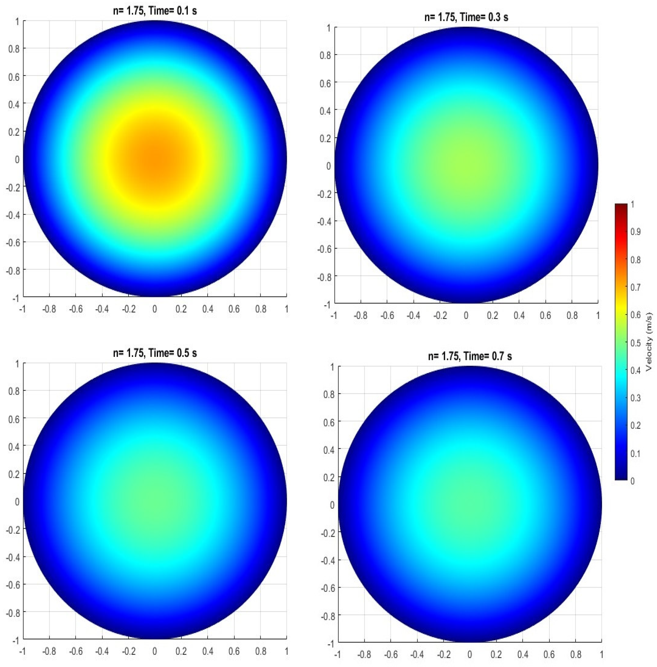
Finally, we illustrate in Figure 5 and Figure 6 the behavior of the unsteady three-dimensional velocity field (46), related to shear-thinning and shear-thickening viscoelastic fluids. The behavior of the solution presented for three-dimensional velocity field $\widehat{\mathit{\vartheta }}$ is associated with the behavior of the volume flow rate solution $\widehat{Q}$ during and after the initial transient phase. We can remark that the shown behavior of the unsteady volume flow rate solution $\widehat{Q}$ has an influence on the choice of time parameters in the illustrations presented in Figure 5 and Figure 6.

4.2. Non-Constant Mean Pressure Gradient

Given the following equation for the non-constant mean pressure gradient

$$\widehat{G}\left(\widehat{t}\right)=1+\frac{{sin}^2\left({\widehat{t}}^2\right)}{e^{\widehat{t}}},$$

(47)

we can verify that it presents a strong variation during the initial transient phase and smaller variation in time after the initial transient phase; see Figure 7.

Let us consider a specific flow regime, i.e., $\widehat{Q}\left(0\right)=1$, ${\widehat{\alpha }}_1=1$, ${\widehat{\beta }}_3=1$ and ${\mathcal{W}}_0=(0.2,0.4,0.6,0.8)$. Using the Runge–Kutta method for solving ordinary differential Equation (43), we can observe the behavior of the unsteady volume flow rate $\widehat{Q}$ for different power index values, related to shear-thinning and shear-thickening viscoelastic fluids; see Figure 8 and Figure 9, respectively. Analyzing the behavior of the volume flow rate illustrated in Figure 8 and Figure 9, we can conclude that, over time, the unsteady solution converges to the steady solution, as in the case where the mean pressure gradient was constant. Also, in these conditions, the convergence is faster for the case of shear-thickening viscoelastic fluid (see Figure 9) than for the shear-thinning case.

Finally, considering the data solution for the unsteady volume flow rate on Equation (46), we can illustrate the behavior of the three-dimensional velocity field (46), related to shear-thinning and shear-thickening viscoelastic fluids; see Figure 10 and Figure 11, respectively. As in the case of a constant mean pressure gradient, the behavior of the solution presented for the three-dimensional velocity field $\widehat{\mathit{\vartheta }}$ is associated with the behavior of the volume flow rate solution $\widehat{Q}$ during and after the initial transient phase. Again, the choice of time parameters in Figure 10 and Figure 11 is associated with the shown behavior of the unsteady volume flow rate solution $\widehat{Q}$ during and after the initial transient phase.

5. Perturbed Flows

When considering the new constitutive Equation (7), we lose the guarantee of stability solution mentioned in condition (5). Therefore, in this section, we intend to take a first approach to the study of the stability solution related to the unsteady volume flow rate $\widehat{Q}$, obtained by the proposed flow model (12). In this sense, we only study the stability solution, where $\widehat{Q}\left(0\right)=1$, ${\mathcal{W}}_0=0.8$, ${\widehat{\alpha }}_1=1$ and ${\widehat{\beta }}_3=1$ are fixed, for different power index parameters.

Now, let us consider the perturbation function, given by

$${\widehat{G}}_{ϵ}^{\pm }=(1\pm ϵ)\widehat{G}$$

(48)

where $ϵ>0$ is the magnitude perturbation and ${\widehat{Q}}_{ϵ}^{\pm }$ is the perturbed volume flow rate related to the perturbation ${\widehat{G}}_{ϵ}^{\pm }$. From the previous section, we know that, over time, the solution to the unsteady volume flow rate $\widehat{Q}$ for constant and non-constant mean pressure gradient converges to the steady solution. As a result, assuming ${\widehat{Q}}_{\widehat{t}}\left(\widehat{t}\right)=0$ in Equation (43), considering specific perturbation ${\widehat{G}}_{ϵ}^{\pm }$, then it is not possible to calculate explicitly the exact expression to the perturbed unsteady volume flow rate ${\widehat{Q}}_{ϵ}^{\pm }$. However, we can overcome this difficulty by calculating the time evolution of the perturbed flow

$$|{\widehat{Q}}_{ϵ}^{+}-{\widehat{Q}}_{ϵ}^{-}|$$

(49)

for fixed magnitude $ϵ>0$.

Consequently, Figure 12 shows the perturbation given by (49) with magnitude $ϵ=0.1$ for shear-thinning and shear-thickening viscoelastic fluid. More properly, Figure 12a illustrates the evolution in time of the perturbation (49) for different power index values, where the mean pressure gradient is constant. In the same way, Figure 12b shows the evolution in time of the perturbation (49) for different power index values, where the mean pressure gradient is non-constant and given by Function (47). Therefore, for specific flow regimes associated with the solutions, we can conclude that, after the initial transition phase, the unsteady volume flow rate behavior is stable in both situations of shear-thinning and shear-thickening viscoelastic fluids.

6. Conclusions

In this work, we proposed a new three-dimensional model for a non-Newtonian incompressible fluid, where viscosity and elasticity vary depending on the shear rate being this dependence a power-law type. The study carried out allowed us to obtain relevant results with applications in different areas of scientific development; for example, in biology, physics, industry, engineering, chemistry, hemodynamics and mathematics. Below, we highlight the main conclusions, namely:

• We obtained the ordinary differential equations involving unsteady mean pressure gradient (unsteady wall shear stress, respectively), unsteady volume flow rate, Womersley number, power index, and material parameters;
• We obtained numerical simulations for the unsteady volume flow rate in specific flow regimes;
• Based on the unsteady solution obtained for the volume flow rate, we presented numerical simulations to the unsteady three-dimensional velocity field in specific flow regimes;
• We presented a study on the perturbed flows.

In addition to the innovation in the proposed model in the field of applications, we highlight the innovative use of Cosserat theory associated with fluid dynamics. This allowed us to move from a three-dimensional model to a one-dimensional model, thus obtaining information about the behavior of the flow volume, which was decisive in the numerical simulations presented for three-dimensional velocity. Finally, for future work, we intend to apply this approximation theory to investigate open problems related to curved tubes and fluid–structure interaction.

References

- Caulk, D.A.; Naghdi, P.M. Axisymmetric motion of a viscous fluid inside a slender surface of revolution. J. Appl. Mech. 1987, 54, 190–196. [Google Scholar] [CrossRef]
- Carapau, F.; Correia, P. One-dimensional Model for Fluids of Third-grade in Tubes with Constant Radius. Int. J. Appl. Math. Stat. 2016, 55, 1–13. [Google Scholar]
- Carapau, F.; Correia, P. Numerical simulations of a third-grade fluid flow on a tube through a contraction. Eur. J. Mech. B/Fluids 2017, 65, 45–53. [Google Scholar] [CrossRef]
- Truesdell, C.; Noll, W. The non-linear field theories of mechanics. In Handbuch der Physik, 3rd ed.; Springer: New York, NY, USA; Berlin/Heidelberg, Germany, 1965. [Google Scholar]
- Rivlin, R.S.; Ericksen, J.L. Stress-deformation relations for isotropic materials. J. Ration. Mech. Anal. 1955, 4, 323–425. [Google Scholar] [CrossRef]
- Fosdick, R.L.; Rajagopal, K.R. Thermodynamics and stability of fluids of third grade. Proc. R. Soc. Lond. A 1980, 339, 351–377. [Google Scholar]
- Beracea, M.; Peati, C.; Simionescu, B.; Navard, P. Shear rheology of semi-dilute poly-methyl-methacrylate solutions. Macromolecules 1993, 26, 7095–7096. [Google Scholar] [CrossRef]
- Mall-Gleissle, S.E.; Gliessle, W.; Mckinley, G.H.; Buggisch, H. The normal stress behavior of suspensions with viscoelastic matrix fluids. Rheol. Acta 2002, 41, 61–76. [Google Scholar] [CrossRef]
- Tao, G.; Otter, W.K.; Briels, W.J. Shear viscosities and normal stress difference in rigid liquid-crystalline polymers. Macromolecules 2006, 39, 5939–5945. [Google Scholar] [CrossRef]
- Coleman, B.D.; Noll, W. An approximation theorem for functionals with applications in continuum mechanics. Arch. Ration. Mech. Anal. 1960, 6, 355–370. [Google Scholar] [CrossRef]
- Chien, S.; Usami, S.; Dellenback, R.J.; Gregerson, M.I.; Nanninga, L.B.; Guest, M.M. Blood Viscosity: Influence of Erythrocyte Aggregation. Science 1967, 157, 829–831. [Google Scholar] [CrossRef]
- Green, A.E.; Naghdi, P.M. A direct theory of viscous fluid flow in channels. Arch. Ration. Mech. Anal. 1984, 86, 39–63. [Google Scholar] [CrossRef]
- Green, A.E.; Naghdi, P.M. A direct theory of viscous fluid flow in pipes I: Basic general developments. Philos. Trans. R. Soc. Lond. A 1993, 342, 525–542. [Google Scholar]
- Green, A.E.; Naghdi, P.M. A direct theory of viscous fluid flow in pipes: II Flow of incompressible viscous fluid in curved pipes. Philos. Trans. R. Soc. Lond. A 1993, 342, 543–572. [Google Scholar]
- Le Roux, C. On flows of third-grade fluids with non-linear slip boundary conditions. Int. J. Non-Linear Mech. 2009, 44, 31–41. [Google Scholar] [CrossRef]
- Akbarzadeh, P. Pulsatile magneto-hydrodynamic blood flows through porous blood vessels using a third grade non-Newtonian fluids model. Comput. Methods Prog. Biomed. 2016, 126, 3–19. [Google Scholar] [CrossRef] [PubMed]
- Almeida, A.; Cipriano, F. Weak Solution for 3D-Stochastic Third Grade Fluid Equations. Water 2020, 12, 3211. [Google Scholar] [CrossRef]
- Guedri, K.; Ahammad, A.N.; Nadeem, S.; Tag-ElDin, E.M.; Awan, A.U.; Yassen, M.F. Insight into the heat transfer of third-grade micropolar fluid over an exponentially stretched surface. Sci. Rep. 2022, 12, 15577. [Google Scholar] [PubMed]
- Nadeem, S.; Ishtiaq, B.; Abbas, N. Impact of thermal radiation on two-dimensional unsteady third-grade fluid flow over a permeable stretching Riga plate. Int. J. Mod. Phys. B 2023, 37, 2350009. [Google Scholar] [CrossRef]
- Swain, S.; Sarkar, G.M.; Sahoo, B. Flow and heat transfer analysis of a special third grade fluid over a stretchable surface in a parallel free stream. Proc. Inst. Mech. Eng. Part C J. Mech. Eng. Sci. 2023, 237, 39–53. [Google Scholar] [CrossRef]
- Jitchote, W.; Robertson, A.M. Flow of second order fluids in curved pipes. J. Non-Newton. Fluid Mech. 2000, 90, 91–116. [Google Scholar] [CrossRef]
- Jordan, P.M.; Puri, P. Stokes first problem for a Rivlin-Ericksen fluid of second grade in a porous half-space. Int. J. Non-Linear Mech. 2003, 38, 1019–1025. [Google Scholar] [CrossRef]
- Massoudi, M.; Phuoc, T.X. Flow of a generalized second grade non-Newtonian fluid with variable viscosity. Contin. Mech. Thermodyn. 2004, 16, 529–538. [Google Scholar] [CrossRef]
- Baranovskii, E.S. Existence results for regularized equations of second-grade fluids with wall slip. Electron. J. Qual. Theory Differ. Equ. 2015, 91, 1–12. [Google Scholar] [CrossRef]
- Das, P.K.; Snider, A.D.; Bhethanabotla, V.R. Acoustic streaming in second-order fluids. Phys. Fluids 2020, 32, 123103. [Google Scholar] [CrossRef]
- Paolucci, S. Second-order constitutive theory of fluids. Contin. Mech. Thermodyn. 2022, 34, 185–215. [Google Scholar] [CrossRef]
- Bhatti, K.; Siddiqui, A.M.; Bano, Z. Application of the second-order fluid model to estimate factors affecting clearance of small and middle uremic molecules using combined ultrafiltration and diffusion processes. Chin. J. Phys. 2023, 86, 458–468. [Google Scholar] [CrossRef]
- Jaffal-Mourtada, B.; Yakoubi, D. A splitting method for a stationary second grade fluid model. AIP Conf. Proc. 2024, 3034, 020017. [Google Scholar] [CrossRef]
- Carapau, F.; Sequeira, A.; Janela, J. 1D simulations of second-grade fluids with shear-dependent viscosity. WSEAS Trans. Math. 2007, 6, 151–158. [Google Scholar]
- Carapau, F. 1D Viscoelastic Flow in a Circular Straight Tube with Variable Radius. Int. J. Appl. Math. Stat. 2010, 10, 20–39. [Google Scholar]
- Carapau, F.; Sequeira, A. Axisymmetric motion of a second order viscous fluid in a circular straight tube under pressure gradients varying exponentially with time. WIT Trans. Eng. Sci. 2006, 52, 409–419. [Google Scholar]
- Robertson, A.M.; Sequeira, A. A director theory approach for modeling blood flow in the arterial system: An alternative to classical 1D models. Math. Models Methods Appl. Sci. 2005, 15, 871–906. [Google Scholar] [CrossRef]
- Carapau, F.; Sequeira, A. 1D Models for Blood Flow in Small Vessels Using the Cosserat Theory. WSEAS Trans. Math. 2006, 5, 54–62. [Google Scholar]
- Womersley, J.R. Method for the calculation of velocity, rate of flow and viscous drag in arteries when the pressure gradient is known. J. Physiol. 1955, 127, 553–563. [Google Scholar] [CrossRef] [PubMed]
Figure 1.
Power-law model for different values of flow index: (a) shear-thinning viscoelastic fluid; (b) shear-thickening viscoelastic fluid.
Figure 2.
Function is the general geometry fluid domain ; functions and , are the normal and tangential components of the surface traction vector, respectively, where is the wall shear stress. Also, is the proximal cross-section, is the distal cross-section, and is the lateral wall of the tube.
Figure 3.
Illustration in time (s) of the volume flow rate (/s) given by (43), where , , , and for shear-thinning viscoelastic fluid, with power index and . (a) Volume flow rate with . (b) Volume flow rate with .
Figure 4.
Illustration in time (s) of the volume flow rate (/s) given by (43), where , , , and for shear-thickening viscoelastic fluid, with power index and . (a) Volume flow rate with . (b) Volume flow rate with .
Figure 5.
Illustration of the three-dimensional velocity (m/s) field (46) over the tube circular cross-section with volume flow rate obtained by (43), where , , , and for shear-thinning fluid with power index . Time (s) parameters: , , , .
Figure 6.
Illustration of the three-dimensional velocity (m/s) field (46) over the tube circular cross-section with volume flow rate obtained by (43), where , , , and for shear-thickening fluid with power index . Time (s) parameters: , , , .
Figure 7.
Mean pressure gradient dependent on time given by (47).
Figure 8.
Illustration in time (s) of the volume flow rate (/s) given by (43), with mean pressure gradient (47), where , , and for shear-thinning viscoelastic fluid, with power index and . (a) Volume flow rate with . (b) Volume flow rate with .
Figure 9.
Illustration in time (s) of the volume flow rate (/s) given by (43), with mean pressure gradient (47), where , , and for shear-thickening viscoelastic fluid, with power index and . (a) Volume flow rate with . (b) Volume flow rate with .
Figure 10.
Illustration of the three-dimensional velocity (m/s) field (46) over the tube circular cross-section, where the volume flow rate is obtained by (43) with mean pressure gradient (47) and , , , for shear-thinning fluid, with power index . Time (s) parameters: , , , .
Figure 11.
Illustration of the three-dimensional velocity (m/s) field (46) over the tube circular cross-section, where the volume flow rate is obtained by (43) with mean pressure gradient (47) and , , , for shear-thickening fluid, with power index . Time (s) parameters: , , , .
Figure 12.
Time (s) evolution of the perturbation (49) with magnitude for shear-thinning and shear-thickening viscoelastic fluid. (a) Constant mean pressure gradient. (b) Non-constant mean pressure gradient.
Disclaimer/Publisher’s Note: The statements, opinions and data contained in all publications are solely those of the individual author(s) and contributor(s) and not of MDPI and/or the editor(s). MDPI and/or the editor(s) disclaim responsibility for any injury to people or property resulting from any ideas, methods, instructions or products referred to in the content. |
© 2024 by the authors. Licensee MDPI, Basel, Switzerland. This article is an open access article distributed under the terms and conditions of the Creative Commons Attribution (CC BY) license (https://creativecommons.org/licenses/by/4.0/).
Share and Cite
MDPI and ACS Style
Carapau, F.; Correia, P.; Rodrigues, G. A Three-Dimensional Velocity Field Related to a Generalized Third-Grade Fluid Model. Mathematics 2024, 12, 1326. https://doi.org/10.3390/math12091326
AMA Style
Carapau F, Correia P, Rodrigues G. A Three-Dimensional Velocity Field Related to a Generalized Third-Grade Fluid Model. Mathematics. 2024; 12(9):1326. https://doi.org/10.3390/math12091326
Chicago/Turabian StyleCarapau, Fernando, Paulo Correia, and Gracino Rodrigues. 2024. "A Three-Dimensional Velocity Field Related to a Generalized Third-Grade Fluid Model" Mathematics 12, no. 9: 1326. https://doi.org/10.3390/math12091326
Note that from the first issue of 2016, this journal uses article numbers instead of page numbers. See further details here.