
Feynman Diagrams beyond Physics: From Biology to Economy


Department of Mathematics, Politecnico di Milano, Via Bonardi 9, Edificio 14 “Nave”, Campus Leonardo, 20133 Milan, Italy
Mathematics 2024, 12(9), 1295; https://doi.org/10.3390/math12091295
Submission received: 18 March 2024
/
Revised: 18 April 2024
/
Accepted: 23 April 2024
/
Published: 25 April 2024
(This article belongs to the Special Issue Algebraic Structures and Graph Theory, 2nd Edition)
Abstract
:Feynman diagrams represent one of the most powerful and fascinating tools developed in theoretical physics in the last century. Introduced within the framework of quantum electrodynamics as a suitable method for computing the amplitude of a physical process, they rapidly became a fundamental mathematical object in quantum field theory. However, their abstract nature seems to suggest a wider usage, which actually exceeds the physical context. Indeed, as mathematical objects, they could simply be considered graphs that depict not only physical quantities but also biological or economic entities. We survey the analytical and algebraic properties of such diagrams to understand their utility in several areas of science, eventually providing some examples of recent applications.
Keywords:
Feynman diagrams; quantum field theory; graph theory; combinatorics; RNA folding; quantum finance; mathematical physicsMSC:
81T18; 81Q30; 81Q65; 91B80; 92-101. Introduction
In the late 1940s, Richard Feynman published a renowned paper [1], in which he proposed a pictorial formulation of the quantum field theory (QFT) by introducing the so-called Feynman diagrams for describing particle interaction as field propagation (see Figure 1). His original attempt was to simplify the tricky computations coming from quantum electrodynamics theory (QED), namely the quantum description of electromagnetic phenomena. As highlighted by David Kaiser [2], the contribution to quantum physics was enormous and, at least, twofold. On the one hand, Feynman diagrams provide a powerful tool to simplify the critical calculations emerging from the perturbative approach in QFT. From this point of view, the diagrams become a topological way to treat enumeration and combinatorical issues. On the other hand, the pedagogical influence that this diagrams had in the second half of the 20th century cannot be overlooked.
The usage of analogous instruments has, not so surprisingly, spread in many other physical field theories. For instance, their application in quantum chromodynamics (QCD) [3,4,5], or even in quantum gravity (QG) [6,7], effective field theory (EFT) [8], and condensed matter physics [9], is quite common nowadays.
There also exists a third philosophical interpretation that considers Feynman diagrams not only merely computational tools, but something that actually provides an in-depth depiction of physical processes [10,11,12]. However, most quantum field theorists actually lean in favour of Feynman diagrams as merely book-keeping devices (namely, they are conveniently employed for calculations) [13,14,15]. In some sense, this work actually shows that, at least as powerful organizational tools, Feynman-type diagrams can be used in different domains not directly linked with quantum phenomena. Indeed, inspired by this intriguing formulation of fundamental physics, namely the graphical description, with its intrinsic topological and algebraic nature, the diagrams began to be used in different domains, such as mathematical biology and economic science. In this manuscript, we survey different applications of Feynman-type diagrams in order to aim at a broad audience, in the hope that these techniques can provide an inspiring starting point for future developments in many scientific areas. We remark that this work fits into the context of a renewed interest in Feynman diagrams, as evidenced by the recent experimentation of their use in a high school setting [16] or the more technical reformulation in categorical semantics [17].
This paper is organized as follows: In Section 2, we briefly introduce the diagrams, stressing their mathematical significance. Section 3 is devoted to the first application of these kinds of graphs in a biological context. A completely different example is given in Section 4, where we review the usage of diagrams in the field of the so-called quantum economy. Finally, in Section 5, we conclude by taking stock of the overview by proposing some other fascinating applications of these particular mathematical tools.
2. From Matrix Integrals to Diagrams
In this section, we propose a brief summary of how diagrams can be generated from a classical mathematical apparatus. There are many authors who discuss the construction of Feynman diagrams and the contextual Feynman rules in QFT [3,5]. In this section, we plan to point out the most important steps in the creation of such graphs, in terms of mathematical operators. Naturally, once you have fixed the graphical apparatus, one can skip the evaluation of the generating functional and the associated Green functions for obtaining amplitudes, as presented in this section. Indeed, the Feynman rules allow us to easily compute the amplitude just by using a list of several formal steps. However, for our purpose, it is important to explain the mathematical formulation behind the diagrams, in order to understand how the same techniques can be used in different scientific domains. Now, we are going to work in a finite-dimensional setting to provide a better explanation of the various passes. Analogous arguments can be found, for instance, in [3,5,18,19,20,21].
As is often the case in mathematics, we start by considering an integral, that is,
where and is a symmetric matrix. After some straightforward computation, it is also possible to prove that, given a generic vector , we can write the following integral:
as
We can now fix a set of k indices as in , so that we can define the so-called k-point function as follows:
This kind of function plays a central role in the development of the theory. Indeed, it is possible to compute Equation (4) by differentiating :
Thus, we immediately obtain the following expression for the one-point function:
and then the generic formulation for the k-points function:
Thanks to these computational steps, we have actually translated the original problem into another one: now, we simply need to compute the derivatives of the exponential function in Equation (3). To reduce this intricate operation to a combinatoric affair, we make use of the well-known Wick’s theorem (which is stated and proved in every book concerning QFT; see, for instance, [5]). In our framework, this theorem immediately leads to a combinatorical expression of the form
With “all parings”, here we denote all possible pairings of the indices . Now, it seems to be clear that the sum of Equation (8) can be split in different contributions by using the N-order series expansion of the exponential function as follows:
In particular, if we use a lighter notation for the derivative, namely
by fixing , we immediately obtain the following from Equation (9):
Let us remark that the paring is equivalent to the paring , because of the symmetry of the matrix . Similarly, for , expressions involve other combinations of indices, for instance,
Thus, Wick’s theorem provides a practical way to compute n-points functions as we show in the latter formulas for the two-points and four-points functions (the generalization is quite obvious). Now, the combinatorial computations arising from Wick’s argument can actually be graphically represented. In particular, let us consider the right-hand side of Equations (12) and (13). They can be depicted as graphs, where the indices of the points in the m-point function become the vertices and and each term becomes an edge from vertex to vertex . Practically speaking, it turns out that it is possible to visualize such an expression by means of graphs, as we propose in Figure 2 and Figure 3.
Remark 1.
The previous paragraphs have explored in depth the link between the mathematical framework and the graphical structures. As mentioned above, the construction of these diagrams can be formulated in a pure formal context by the list of Feynman rules. The latter formulation really provides an easier way to construct the diagrams. However, as we are going to see in the next sections, the mathematical background represents one of the cores of this work, which one needs in order to have a better understanding of the translation of these techniques in other studies.
Physically speaking, the structure of Feynman diagrams arises directly from the integrals (namely the generating function) due to the path integral approach to QFT [5]. In fact, in the quantum field theory realm the studied integrals assume (by adapting the previous notations) the following form, which involves some potential function and the reduced Planck constant ℏ:
Equation (14) is trivially linked with the above discussion (we remark that the construction in QFT is actually more complicated, as it involves infinite quantities. However, for the purpose of this illustrative section, the most important thing is to capture the spirit of the mathematical formulation linked to Feynman diagrams). Now, as one can deduce from the proposed construction, it is possible to fix some formal rules in order to connect this abstract mathematical formulation to the corresponding physical significance. This procedure imposes the classical QED interpretation first provided by Feynman (and formally developed by Dyson [22]), in which objects as virtual particles are introduced in order to explain the physical phenomena underlying the diagrams (the ontological nature of virtual particles is still an open debate in the philosophical community [23,24]). However, for the purpose of this work, we just consider the mathematical formulation of such diagrams and how their generality can be translated to other scientific domains. Indeed, in this section, we show how it is possible to construct a graph theory starting from a specific class of integrals.
In the next two sections, we apply this impressive trick coming from QFT to develop a graph theory for approaching the problem of RNA folding and for modelling the bond prices in quantum finance.
Remark 2.
It is important to underline that the application of diagrams in the biological and economical contexts actually comes from two different perspectives. In fact, in the first case, the analogy inspiring the construction comes, as we are going to see, directly from the similarity between the pictures in the QFT and RNA framework. Instead, in the second case, the analogy is mediated by the path integral formulation. It is now quite clear that the formal mathematical construction can be based directly on the path integral formulation instead of its diagrammatic version. However, we consider the choice of Feynman-type diagrams for developing and studying the most suitable theories in order to disseminate such an approach to different scientific communities. For the role of the analogy in the mathematical reasoning and discovery, we refer interested readers to [25,26].
3. RNA Folding Problem
In the previous section, we formally show the connection between matrices and diagrams. This deep link can be exploited to study many kinds of problems once one has reformulated the link in terms of matrix field theory. In this spirit, in 2002 Orland and Zee [27] proposed a method for predicting the tertiary structure of RNA based on such a matrix theory. Indeed, the usage of diagrams to describe secondary and tertiary RNA structures is actually a common practice, as testified by a large number of representations, which one can find in the literature [27,28,29,30,31,32,33,34,35].
We briefly recall that RNA is usually defined as a single-filament polymer, made of ribonucleosides with four main nucleobases: adenine (A), cytosine (C), guanine (G), and uracil (U). Despite being single-filament, RNA bases can form bonds (similarly to DNA) with bases from other molecules, or even within the same molecule, thus creating more complicated 2D and 3D structures. In standard Watson–Crick base-pairings, A binds U with two hydrogen bonds, and G binds C with three hydrogen bonds. Moreover, RNA structural motifs are made up of two components: the first one consists of free bases, like in bulges, loops, or junctions, and the second one is made up of stems of paired bases. While the secondary structure could be assimilated to RNA’s planar conformation (i.e., planar graphs), the tertiary structure is its 3D conformation, which determines its specific function (see [36]). The main role in the passage between 2D and 3D models is played by the so-called pseudoknots. Roughly speaking, a pseudoknot is composed of at least two helices with both internal bonds and free bases interacting across the two motifs and separated by an additional stretch of free bases (see [37]). In the next paragraphs, we explore in-depth the contribution of pseudoknots in this framework and their graph representation.
Returning to the main topic, Orland and Zee noticed a profound analogy between the model obtained by stretching the manipulation of RNA secondary structures (see Figure 4) and the classical Feynman diagrams defined above.
It turns out that such an approach is strictly related to the topology of such diagrams, as it was already proved by t’Hooft [38]. Thanks to this topological perspective, we can introduce the fundamental notion of genus, which can be used to topologically classify RNA structures [30,32,33,39]. It is important to underline that the formal construction, which we are going to explain in the following, is none other than a particular case of a the so-called maps enumeration problem belonging to the theory of dessin d’enfant, whose contemporary formulation in terms of graph embedding into manifolds is due to Grothendieck [40]. Readers interested in the latter topic may also consult the manuscript published by Zvonkin [41]. The matrix formalism introduced in [27] and then developed in [32] is based on the standard energy models for RNA studied in recent years. These energetic models are based on the following partition function:
where is the 3D position vector k-th base, L is the length of the sequence, and is a function, which takes into account the properties of the RNA chain. A fundamental role is played by the function , which provides the description of base interactions; it is given by
where denotes the pair relation , the quadruplets relation , and so on. In this formalism, the function represents the Boltzmann factor with energy that relates the i-th and the j-th bases at the distance induced by the vector :
where is the usual symbol for the inverse temperature multiplied to the Boltzmann constant, and is the space-dependent part of the interaction. And, precisely in this context, Orland and Zee noticed the analogy with QCD that induced them to rewrite the above problem in terms of integrals over the space of dimensional Hermitian matrices:
where is a Hermitian matrix, represents the trace operator, and is a computable normalization factor.
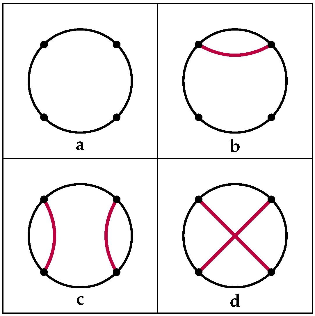
These latter integrals can be represented by means of diagrams inspired by the Feynman diagrams that we introduced in the previous section. Let us consider for the sake of simplicity the one-dimensional case (), with . By basic computations, we obtain , namely, if one depicts a circle with two points, the addendum 1 is the no-chord diagram, and the term a is the diagram with chords joining the two points. Now, it is also possible to represent , where, in addition to the no-chord diagram, there are also six one-chord diagrams (all the possible combinations) that provide the term . Finally, are intuitively the three possible combinations of two-chord diagrams (see Figure 5 for some examples).
Remark 3.
As we are going to explain in the next paragraphs, the power of this approach becomes relevant for large N and large expansion. In particular, one can notice that the computation of does not depend on N; instead, by computing , one explicitly obtains the dependence on N. We remark that, in this example, the term involving actually represents the non-planar diagram.
Once the matrix framework is recovered, it is possible to evaluate such integrals in terms of diagrams, by using the already mentioned Wick’s theorem. Moreover, thanks to this graphical approach we can also describe pseudoknots in terms of topological quantities, namely the genus. Figure 4 depicts the standard way to represent a well-known pseudoknot, called kissing hairpin [42]. This picture can be used to derive (by stretching the backbone) two other useful graphs, namely the stretching (or arc) diagram (Figure 6a) and the circle (or disk) diagram (Figure 6b).
Now, in terms of crossing diagrams, pseudoknots can be computed by using the genus of a surface. Topologically speaking, the genus of a surface is the number of holes or handles of a (orientable) surface. In this framework, the genus of a diagram can be defined as the genus of the surface with the lowest genus, in which our diagram can be drawn with no intersections. In particular, if we consider the case of the kissing hairpin, we obtain the representation in Figure 7, in which the diagram appears embedded in a surface with genus , namely a torus.
It is clear now how the topology allows us to classify pseudoknots, which have a central role in the theory. We remark, indeed, that the genus g is included explicitly in the original formulation of the theory [27,32,43], in which the authors consider power series of Equation (18) with respect to terms of the form (where N is the dimension of the matrix), so that Equation (16) can be rewritten by also including the topological contribution due to pseudoknots (we can assume that the chains are infinitely flexible, so that all spatial degrees of freedom are gotten rid of when simplifying the notation):
Remark 4.
We point out that Equation (19) explicitly provides the link between secondary and pseudoknot structures from a topological perspective. In particular, the topological considerations that lead to Equation (19) are based on the N expansion used in the already mentioned matrix field theories. Indeed, this approach predicts that non-planar Feynman diagrams have amplitudes proportional to the negative power of N, and then we can get rid of them when N is large. The same technique has been applied to the problem of RNA folding, leading to the same sort of cancellation of non-planar configurations [27].
The standard way to compute the genus of a diagram is the well-known Euler characteristic that, in the case of diagrams, is provided by the celebrated formula , where , and F are the numbers of vertices, edges, and faces, respectively. We remark that, in this view, a vertex is a nucleotide, an edge is any line connecting two nucleotides, and a face is a part of the surface within a closed loop of edges. In the case of n arcs, one trivially obtains . There is also a famous theorem due to Euler stating that any polyhedron homeomorphic to a sphere with a boundary has an Euler characteristic . As a corollary, all RNA secondary structures with no pseudoknots can be represented by disk diagrams with . Let us suppose that the RNA secondary structure admits pseudoknots; as in the case of kissing hairpin, the computation of the Euler characteristic leads to the value . The geometrical significance of such a value is strictly related to the number of holes on a surface. In particular, we recall that for any orientable surface, we have , where p is the number of punctures. In conclusion, the kissing hairpin pseudoknot induces a genus , and can be drawn without crossing on a surface with one hole, that is exactly a torus (Figure 7).
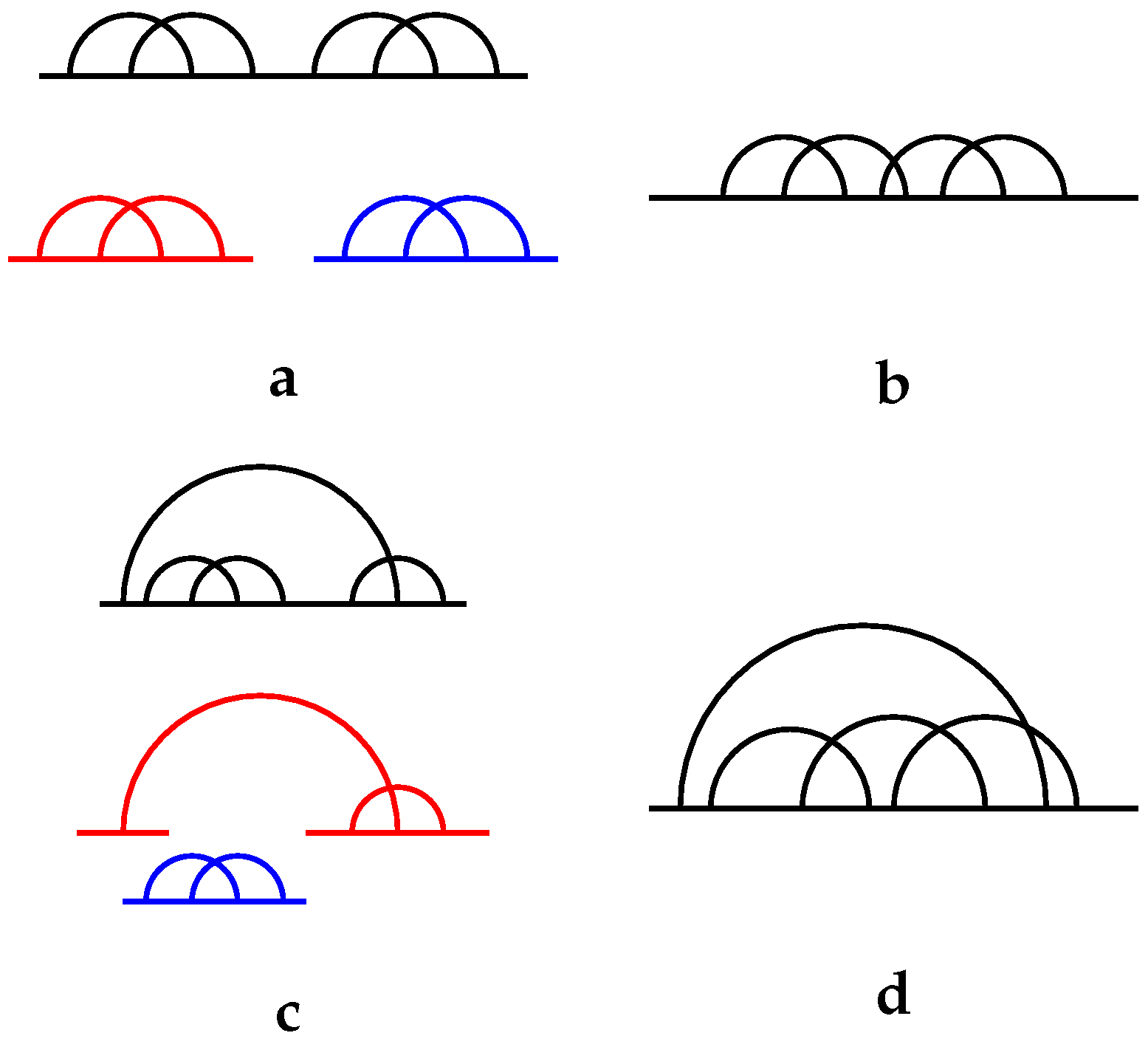
Now, we want to stress two more properties about pseudoknots that turn out to be very important for computational reasons. The genus of a diagram is an additive quantity, and so it is possible to provide two notions to characterize the intrinsic complexity of a pseudoknot, namely the concepts of irreducibility and nested pseudoknots [42]. A diagram is said to be irreducible if it cannot be split into two disconnected parts by cutting a single line, as in Figure 8b. In parallel, a diagram is said to be nested in another one if it can be removed by cutting two lines and keeping the rest of the diagram connected in a single component, as in Figure 8d. These two definitions can be combined as follows: if a diagram is both irreducible and non-nested, it is called a primitive diagram. Other interesting details about genuses and pseudoknots can be found in [32,33,39,42,44].
Remark 5.
This section is devoted to the explanation of how the matrix theory can be applied in the context of RNA folding prediction problems and the way to connect pseudoknots with genuses by using graphs and their embedding into manifolds. The interests for this method assume a greater significance when such an approach is used to developed specific software for modelling and predicting RNA structures. In particular, we want to mention McGenus [45] and its precursor TT2NE [46]. Indeed, the notion of pseudoknots and the graphical apparatus outlined above allow us to consider, in producing a suitable predictive software, having both the perspectives: the global one (provided by genuses and pseudoknots) and the local one (provided by the energy function due to the coupling rules of the biological theory). A useful overview about these topics and the most recent applications of McGenus is eventually proposed in [47].
For the sake of completeness, finally, we want to mention some other recent works that describe a topological approach based on graphs to RNA folding problems. A similar outlook to the one described above is given in [28], where the authors studied a Hermitian matrix model with a given potential that enumerates the number of chord diagrams by using the formalism of the topological recursion, and in [29], where the authors provided a classification and an enumeration of RNA structures by genus. Moreover, two interesting generalizations of the concept of genuses were introduced [31,35]. The first one is the genus trace, a function providing the genus of a segment of the chain between the first and the i-th residue. The second one is the fingerprint matrix, which gives a useful mathematical visualization of all the genuses computed between two elements of a chain; namely, if one fixes the notation for the matrix, the generic element represents the genus of the sub-chain between the i-th and the j-th residue. Another computational approach based on pseudoknot prediction is given in [34], where the authors proposed a quantitative analysis of the topological constraints on RNA three-dimensional conformational space, with specific attention to the distribution of helix orientations, for pseudoknots and loop–loop kissing structures. The results showed a strong topological coupling between helices and loops in RNA tertiary motifs.
4. Quantum Finance Experience
In this fourth section, we describe a completely different application of Feynman-type diagrams in the interdisciplinary field of econophysics [48,49,50]. In general, this field of study exploit methods and approaches developed in the domain of physics to solve economical and financial problems.
In the following paragraphs, we focus on an intriguing topic, which is based on quantum theories, and therefore it is called quantum econophysics. Although there are several doubts about the ontological foundation of the analogy between quantum mechanics and finance [51], it is still interesting to describe the framework proposed by several authors in the last two decades based on the path integral formulation, which can even be reformulated with the graphical techniques introduced by Feynman and discussed in Section 2. The first attempt to merge quantum and economic theory dates back to the end of the 1970s with the first works of Qadir [52] and Samuelson [53]. Specifically, the first one proposed, under suitable assumptions, the use of quantum formalism to model micro-economics (in analogy with micro-physics). A renewed interest in these ideas started to emerge between the end of the 1990s and the beginning of the 2000s, thanks to researchers coming from the social sciences such as Shubik [54] and Haven [55].
However, at the same time, the two most important approaches to quantum econophysics came onto the stage, that is, the works of Ilinski [56] and Baaquie [57]. In the following years, Baaquie has considerably developed his own approach with several manuscripts [58,59,60,61,62] and books [63,64], which represent the core of this section. Interested readers can find further materials on quantum methods for economics and finance in [65,66,67,68,69]. In the following paragraphs, we explore the formalism developed by Baaquie [57,59,70] for modelling European options on coupon bonds.
Remark 6.
European options represent the most used path-independent options. An option is said to be path-independent if the payoff function is independent of how the security arrives at its final price. On the contrary, path-dependent options (such as American or Asian options) are ones in which payoff functions depend on the whole path that the security takes before the option expires. For further details, see [57,71]. Moreover, we recall that a bond is a primary negotiable financial instrument that at the pre-established maturity gives its owner the right to repayment of the capital lent to the issuer plus a fixed or variable interest rate, the coupon (basically, it is a special type of investment). A derivative financial instrument is instead the option, which gives to the owner the possibility to buy or sell the underlying bond at a certain price on or before the option expiry date.
The formalism introduced by Baaquie is inspired by QFT and it naturally leads to Feynman representation of a perturbative series, which, in this case, models a financial instrument, namely the forward interest rate (the forward interest rate is just the future yield on a coupon bond). More formally [70], we can denote by the function representing the forward interest rates for a fixed time t and a loan at some future times . With this notation, it is possible to define the forward price of a bond (maturing at time ) in terms of the interest rate:
where is the future time (with respect to the initial time ) for which a zero coupon bond is going to be issued. The development of a rigorous mathematical formulation of the forward interest rates starts from the following equation that describes the time evolution of such rates :
where denotes the two-dimensional quantum field (a stochastic random field) associated with the forward interest rates, is the drift fixed by a choice of numeraire, and is the volatility given by the market itself. In this context, one can consider and as two-dimensional quantum fields [70]. In this framework, it is possible to express the quantum field theory of the forward interest rates thanks to the following generating function [57]:
where the stiff action S and the partition function Z are, respectively,
Here, denotes a suitable Lagrangian describing the evolution of instantaneous forward rates depending on the three parameters, as explained in [57].
Now, following the argument in [59], in the case of (European) options for coupon bonds, the price of the call option has a partition function of the form
where Z was already defined in Equation (23), and V is the so-called notional principal amount. Mathematically speaking, the price at time t of a Treasury Bond maturing at some future time can be defined by using the forward interest rates as
As explained in [59], it is also possible to rewrite the price of the coupon bond in terms of a zero coupon bond and the interest rate , defined in Equation (20) as
Here, denotes (fixed) dividends payed at time , for . Moreover, in these settings, one can prove (see [70]) that V is actually a small perturbation of F.
As highlighted by Baaquie [57], the volatility of the forward interest rates is actually a little quantity, namely it is approximately /year. Thus, the volatility function can be used as a perturbation, that is, an expansion parameter, and the approximation of the partition function can be systematically improved by expanding to higher orders. In other words, the goal now becomes the construction of an analytical expression that yields the price of the coupon bond option in terms of the power series (in ) of the partition function given in Equation (24). The analogy with QFT is exploited to develop the rigorous perturbation expansion for the partition function, whose terms can be computed in terms of Feynman diagrams. In particular, we have the following cumulant expansion:
where the parameters are computed thanks to the Feynman diagram representations. There is now a technical–financial hypothesis to add on our argument, namely the put–call parity constraint. Roughly speaking, put–call parity is a relationship between the price of a call option and a put option, which mathematically leads to the following conditions:
This imposes , and it leads to the simplified version of Equation (25):
It is possible to expand the partition function even in a power series in . Such an expansion yields to
By comparing Equations (26) and (27), it is possible to find the relation between the coefficients , , and V (see also Remarks 7 and 8). Remarkably, one can see that the martingale condition implies that , so that put–call parity is satisfied. Moreover, these coefficients can be described more specifically by introducing a suitable correlation function (a real symmetric matrix) for expressing the correlation in the fluctuations of the forward bond prices and . If we denote the magnitude of the matrix elements as G and use the relation , we can rewrite partition function as
where the coefficients are . Here, the quadratic term in the exponential for Z fixes the magnitude of the perturbations as . As a consequence, the remaining terms are of order , , and so on. This argument allows us to compute the partition function to any order of accuracy with respect to the parameter G (or, equivalently, ).
Remark 7.
In the previous paragraphs, we described the construction of the series expansion of the partition function . It is now clear that the next step involves the computation of the following coefficients emerging from the comparisons of Equations (26) and (27), namely the following (we recall that the coefficient has to be 0 because of the put–call parity condition):
The analytic computation of these values is given in full in Appendix of [59].
Once we fix this formalism, it appears quite natural to connect the perturbative expansion of the partition function Z with the Feynman diagrams. Specifically, the forward bond propagator that denotes the correlation between the forward bond price and can be depicted with a wavy line as in Figure 9.
This graph formalism can be used to compute the coefficients , , and of Equation (27) as represented in Figure 10.
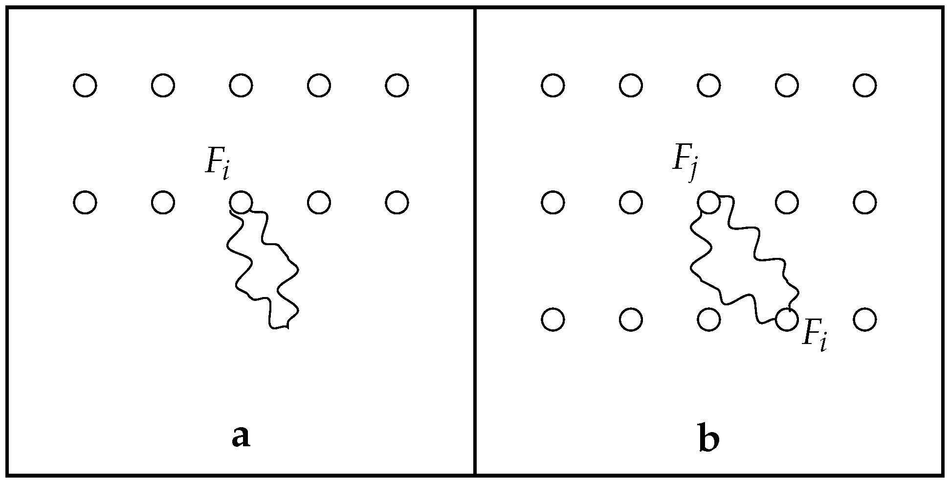
We remark that all the diagrams contributing in the series of the partition function Z are connected, namely none of the forward bond prices are decoupled from the forward bond propagator . However, it is also possible to produce disconnected Feynman diagrams (that do not contribute to any of the coefficients), as one can see in Figure 11.
The application of Feynman pictorialism in modelling financial objects represents an intriguing possibility for using such a formalism in a practical framework. In particular, it is interesting to underline that such a theoretical construction has a corresponding empirical study, which can be found in [62]. Apart from the interpretive aspects that surely represent a non trivial issue, the visualization of the terms arising from the series expansion (28) by means of Feynman-type diagrams provides a powerful tool, in order to compute the price of the option for a coupon bond in the framework of quantum finance. However, the works mentioned above can be considered the first technical step in a wider study in this fascinating field.
Remark 8.
The computations of Remark 7 are summarized by the graphs represented in Figure 10. In particular, by some intricate calculations (see Appendix of [59]), it is possible to obtain the following expression for the coefficient depending on the propagator :
where and , with . Thus, by expanding the exponential functions, we obtain
which is equivalent to the Feynman-type representation in Figure 10a. Analogous expressions can be found also for coefficients and , which are equivalent to the graphs in Figure 10b and Figure 10c, respectively.
5. Conclusions
In this work, we have presented two different applications of the Feynman diagrammatic formalism belonging to two completely different domains. On the one hand, RNA secondary and tertiary structures can be modelled intuitively in terms of graphs by involving the matrix theory as theoretical support. On the other hand, the field of econophysics, based on the path integral formulation of the theory, finds a strong ally for studying nonlocal and nonlinear problems.
The abstract nature of the mathematics behind Feynman diagrams suggest the wider use of these tools, which actually transcends the original physical domain. Indeed, we remark that the mathematical significance of Feynman diagrams is well studied in terms of algebraic lattice structures in the framework of Hopf algebras [72,73] and tensor models [74].
In this concluding section, we want to propose a few more attempts to use Feynman diagrams in unusual scientific areas of study. One of the most natural applications of Feynman diagrams has arisen in geophysics for modelling different scenarios involving wave propagation. In this field, we indicate, by way of example, two interesting works. The first one regards wave propagation in a laterally heterogeneous medium [75]. Here, the authors used diagrams to find a solution for random media elastic wave problems involving Dyson’s equation and the Bethe–Salpeter equation. The second study exploits the closer link between the perturbation graphs and collision diagrams for modelling scattering processes in oceanic wave guides involving surface and internal gravity waves [76].
Other stimulating employments of Feynman-type graphs come from the field of chemistry, where this kind of representation is used to derive a more accurate reaction–diffusion equation starting from a path integral formulation [77], or even for the so-called 2D-Raman-THz spectroscopy of liquid water [78].
A fascinating arrangement of Feynman diagrams is given in information theory for distributed quantities, which actually provides a Bayesian statistical field theory named information field theory. In this framework, interacting information field theories can be diagrammatically expanded in terms of Feynman diagrams [79,80].
Finally, we mention three different applications in the medical area. In the first case, the authors proposed a method for studying some neuronal function signal propagations based on the cable equation [81]. The benefit of this approach is the possibility of working with Green’s function, corresponding to the propagator of the system that may be handled with techniques employed in the many body systems theory and then represented by Feynman diagrams. The second case aimed to investigate brain function by using electroencephalogram (EEG) combined with a set of Feynman rules inspired by quantum particle interactions [82]. In particular, the author introduces the brain state matrix, which is composed of several EEG indicators, for predicting several brain reactions that are analyzed as sensory-evoked and event-related potentials. The last medical example regards cardiac arrhythmia. In [83], the authors introduced three quasiparticles (heads, tails, and pivots) in order to capture the rich dynamics in excitable systems (which are a large class of chemical and biological systems). Specifically, they used Feynman-like diagrams to represent the dynamical creation, annihilation, and recombination of the identified quasiparticles.
As we have seen in this paper, the usage of Feynman diagrams, as powerful computational tools, seems to go beyond the original physical setting. The graphical approach that many satisfactions gave to QED has an intrinsic capacity to reproduce complicated abstract concepts (such as matrix integrals) in a more suitable and intuitive way. We hope that such a work could be good inspiration for researchers coming from different scientific areas who want to look at things from a different and fascinating angle.
Funding
This research received no external funding.
Acknowledgments
The author would like to express his gratitude to Gianni Arioli and Giovanni Valente for the numerous discussions on the interpretation of Feynman diagrams. Many thanks also to Jacopo Cangiotti, Marco Capolli, Stefano Grasso, and Mattia Sensi for their precious support and important suggestions to improve this work. The author is a member and acknowledges the support of Gruppo Nazionale per l’Analisi Matematica, la Probabilità e le loro Applicazioni (GNAMPA) of Istituto Nazionale di Alta Matematica (INdAM), and, moreover, acknowledges the support of the MIUR—PRIN 2022 project “Nonlinear dispersive equations in presence of singularities” (Prot. N. 20225ATSTP). Finally, the author thanks the anonymous reviewers for their careful reading of the manuscript and their many insightful comments and suggestions.
Conflicts of Interest
The author declares no conflicts of interest.
References
- Feynman, R.P. Space-Time Approach to Quantum Electrodynamics. Phys. Rev. 1949, 76, 769–789. [Google Scholar] [CrossRef]
- Kaiser, D. Drawing Theories Apart: The Dispersion of Feynman Diagrams in Postwar Physics; University of Chicago Press: Chicago, IL, USA, 2005. [Google Scholar]
- Griffiths, D. Introduction to Elementary Particles; Harper & Row: New York, NY, USA, 1987. [Google Scholar]
- Mangano, M.L. Introduction to QCD. In Proceedings of the 1998 European School of High-Energy Physics, St. Andrews, UK, 23 August–5 September 1998; pp. 53–97. [Google Scholar]
- Peskin, M.E.; Schroeder, D.V. An Introduction to Quantum Field Theory; Westview Press: New York, NY, USA, 1995. [Google Scholar]
- Barrett, J.W. Feynman diagrams coupled to three-dimensional quantum gravity. Class. Quantum Gravity 2006, 23, 137–141. [Google Scholar] [CrossRef]
- Reisenberger, M.P.; Rovelli, C. Spacetime as a Feynman diagram: The connection formulation. Class. Quantum Gravity 2001, 18, 121–140. [Google Scholar] [CrossRef]
- Goldberger, W.D.; Rothstein, I.Z. Effective field theory of gravity for extended objects. Phys. Rev. D 2006, 73, 104029. [Google Scholar] [CrossRef]
- Jishi, R.A. Feynman Diagram Techniques in Condensed Matter Physics; Cambridge University Press: Cambridge, UK, 2013. [Google Scholar]
- Meynell, L. Why Feynman diagrams represent. Int. Stud. Philos. Sci. 2008, 22, 39–59. [Google Scholar] [CrossRef]
- Stöltzner, M. Feynman Diagrams as Models. Math. Intell. 2017, 39, 46–54. [Google Scholar] [CrossRef]
- Stöltzner, M. Feynman Diagrams: Modelling between Physics and Mathematics. Perspect. Sci. 2018, 26, 482–500. [Google Scholar] [CrossRef]
- Dorato, M.; Rossanese, E. The Nature of Representation in Feynman Diagrams. Perspect. Sci. 2018, 26, 443–458. [Google Scholar] [CrossRef]
- Passon, O. On the interpretation of Feynman diagrams, or, did the LHC experiments observe H → γγ? Eur. J. Philos. 2019, 9, 20. [Google Scholar] [CrossRef]
- Redhead, M. Models in physics. Br. J. Philos. Sci. 1980, 31, 145–163. [Google Scholar] [CrossRef]
- Dahlkemper, M.N.; Klein, P.; Müller, A.; Schmeling, S.M.; Wiener, J. Opportunities and Challenges of Using Feynman Diagrams with Upper Secondary Students. Physics 2022, 4, 1331–1347. [Google Scholar] [CrossRef]
- Shaikh, R.A.; Gogioso, S. Categorical Semantics for Feynman Diagrams. arXiv 2022, arXiv:2205.00466. [Google Scholar]
- Polyak, M. Feynman diagrams for pedestrians and mathematicians. Graphs Patterns Math. Theor. Phys. 2005, 73, 15–42. [Google Scholar]
- Srednicki, M. Quantum Field Theory; Cambridge University Press: Cambridge, UK, 2007. [Google Scholar]
- Ticciati, R. Quantum Field Theory for Mathematicians; Cambridge University Press: Cambridge UK, 1999. [Google Scholar]
- Wüthrich, A. The Genesis of Feynman Diagrams; Springer: Berlin/Heidelberg, Germany, 2016. [Google Scholar]
- Dyson, F.J. Divergence of perturbation theory in quantum electrodynamics. Phys. Rev. 1952, 85, 631–632. [Google Scholar] [CrossRef]
- Fox, T. Haunted by the Spectre of Virtual Particles: A Philosophical Reconsideration. J. Gen. Philos. Sci. 2008, 39, 35–51. [Google Scholar] [CrossRef]
- Jaeger, G. Are Virtual Particles Less Real? Entropy 2019, 21, 141. [Google Scholar] [CrossRef] [PubMed]
- Cangiotti, N.; Nappo, F. Reasoning by Analogy in Mathematical Practice. Philos. Math. 2023, 31, 176–215. [Google Scholar] [CrossRef]
- Nappo, F.; Cangiotti, N.; Sisti, C. Confirming Mathematical Conjectures by Analogy. Erkenntnis, 2023; Online First Articles. [Google Scholar]
- Orland, H.; Zee, A. RNA folding and large N matrix theory. Nucl. Phys. B 2002, 620, 456–476. [Google Scholar] [CrossRef]
- Andersen, J.E.; Chekhov, L.O.; Penner, R.C.; Reidys, C.M.; Sułkowski, P. Topological recursion for chord diagrams, RNA complexes, and cells in moduli spaces. Nucl. Phys. B 2013, 866, 414–443. [Google Scholar] [CrossRef]
- Andersen, J.E.; Penner, R.C.; Reidys, C.M.; Waterman, M.S. Topological classification and enumeration of RNA structures by genus. J. Math. Biol. 2013, 67, 1261–1278. [Google Scholar] [CrossRef]
- Pillsbury, M.; Orland, H.; Zee, A. Steepest descent calculation of RNA pseudoknots. Phys. Rev. E 2005, 72, 011911. [Google Scholar] [CrossRef] [PubMed]
- Rubach, P.; Zajac, S.; Jastrzebski, B.; Sulkowska, J.I.; Sułkowski, P. Genus for biomolecules. Nucleic Acids Res. 2019, 48, D1129–D1135. [Google Scholar] [CrossRef]
- Vernizzi, G.; Orland, H.; Zee, A. Enumeration of RNA structures by matrix models. Phys. Rev. Lett. 2005, 94, 168103. [Google Scholar] [CrossRef] [PubMed]
- Vernizzi, G.; Ribeca, P.; Orl, H.; Zee, A. Topology of pseudoknotted homopolymers. Phys. Rev. E 2006, 73, 031902. [Google Scholar] [CrossRef] [PubMed]
- Xu, X.; Chen, S.-J. Topological constraints of RNA pseudoknotted and loop-kissing motifs: Applications to three-dimensional structure prediction. Nucleic Acids Res. 2020, 48, 6503–6512. [Google Scholar] [CrossRef] [PubMed]
- Zając, S.; Geary, C.; Andersen, E.S.; Dabrowski-Tumanski, P.; Sulkowska, J.I.; Sułkowski, P. Genus trace reveals the topological complexity and domain structure of biomolecules. Sci. Rep. 2018, 8, 17537. [Google Scholar] [CrossRef] [PubMed]
- Antczak, M.; Popenda, M.; Zok, T.; Zurkowski, M.; Adamiak, R.W.; Szachniuk, M. New algorithms to represent complex pseudoknotted RNA structures in dot-bracket notation. Bioinformatics 2017, 34, 1304–1312. [Google Scholar] [CrossRef]
- ten Dam, E.; Pleij, K.; Draper, D. Structural and functional aspects of RNA pseudoknots. Biochemistry 1992, 31, 11665–11676. [Google Scholar] [CrossRef]
- ’t Hooft, G. A planar diagram theory for strong interactions. Nucl. Phys. B 1974, 72, 461–473. [Google Scholar] [CrossRef]
- Vernizzi, G.; Orland, H.; Zee, A. Classification and predictions of RNA pseudoknots based on topological invariants. Phys. Rev. E 2016, 94, 042410. [Google Scholar] [CrossRef]
- Grothendieck, A. Geometric Galois Action 1; London Mathematical Society Lecture Note Series; Chapter Esquisse d’un Programme; Cambridge University Press: Cambridge, UK, 1997; Volume 242, pp. 5–48. [Google Scholar]
- Zvonkin, A. Matrix integrals and map enumeration: An accessible introduction. Math. Comput. Model. 1997, 26, 281–304. [Google Scholar] [CrossRef]
- Bon, M.; Vernizzi, G.; Orl, H.; Zee, A. Topological classification of RNA structures. J. Mol. Biol. 2008, 379, 900–911. [Google Scholar] [CrossRef] [PubMed]
- Vernizzi, G.; Orland, H.; Zee, A. Prediction of RNA pseudoknots by Monte Carlo simulations. arXiv 2004, arXiv:q-bio/0405014. [Google Scholar]
- Bon, M.; Orl, H. Prediction of RNA secondary structures with pseudoknots. Phys. A Stat. Mech. Appl. 2010, 389, 2987–2992. [Google Scholar] [CrossRef]
- Bon, M.; Micheletti, C.; Orland, H. McGenus: A Monte Carlo algorithm to predict RNA secondary structures with pseudoknots. Nucleic Acids Res. 2012, 41, 1895–1900. [Google Scholar] [CrossRef] [PubMed]
- Bon, M.; Orland, H. TT2NE: A novel algorithm to predict RNA secondary structures with pseudoknots. Nucleic Acids Res. 2011, 39, e93. [Google Scholar] [CrossRef]
- Cangiotti, N.; Grasso, S. Genus Comparisons in the Topological Analysis of RNA Structures. arXiv 2023, arXiv:2304.07273. [Google Scholar]
- Dash, K.C. The Story of Econophysics; Cambridge Scholars Publishing: Newcastle upon Tyne, UK, 2019. [Google Scholar]
- Jovanovic, F.; Schinckus, C. Econophysics and Financial Economics: An Emerging Dialogue; Oxford University Press: Oxford, UK, 2017. [Google Scholar]
- Mantegna, R.N.; Stanley, H.E. Introduction to Econophysics: Correlations and Complexity in Finance; Cambridge University Press: Cambridge UK, 1999. [Google Scholar]
- Arioli, G.; Giovanni, V. What Is Really Quantum in Quantum Econophysics? Philos. Sci. 2021, 88, 665–685. [Google Scholar] [CrossRef]
- Qadir, A. Quantum Economics. Pak. Econ. Soc. Rev. 1978, 16, 117–126. [Google Scholar]
- Samuelson, P. A quantum theory model of economics: Is the co-ordinating entrepreneur just worth his profit? In The Collected Scientific Papers of Paul A. Samuelson; The MIT Press: Cambridge, MA, USA, 1999; Volume 4. [Google Scholar]
- Shubik, M. Quantum economics, uncertainty and the optimal grid size. Econ. Lett. 1999, 64, 277–278. [Google Scholar] [CrossRef]
- Haven, E. A discussion on embedding the Black–Scholes option pricing model in a quantum physics setting. Phys. A Stat. Mech. 2002, 304, 507–524. [Google Scholar] [CrossRef]
- Ilinski, K. Physics of Finance: Gauge Modelling in Non-Equilibrium Pricing; John Wiley & Sons Inc.: Hoboken, NJ, USA, 2001. [Google Scholar]
- Baaquie, B.E. Quantum Finance—Path Integrals and Hamiltonians for Options and Interest Rates; Cambridge University Press: Cambridge, UK, 2004. [Google Scholar]
- Baaquie, B.E. A Common Market Measure for Libor and Pricing Caps, Floors and Swaps in a Field Theory of forward Interest Rates. Int. J. Theor. Appl. Financ. 2005, 8, 999–1018. [Google Scholar] [CrossRef]
- Baaquie, B.E. Feynman perturbation expansion for the price of coupon bond options and swaptions in quantum finance. I. Theory. Phys. Rev. E 2007, 75, 016703. [Google Scholar] [CrossRef] [PubMed]
- Baaquie, B.E. Action with Acceleration I: Euclidean Hamiltonian and Path Integral. Int. J. Mod. Phys. A 2013, 28, 1350137. [Google Scholar] [CrossRef]
- Baaquie, B.E. Action with Acceleration II: Euclidean Hamiltonian and Jordan Blocks. Int. J. Mod. Phys. A 2013, 28, 1350138. [Google Scholar] [CrossRef]
- Baaquie, B.E.; Liang, C. Feynman perturbation expansion for the price of coupon bond options and swaptions in quantum finance. II. Empirical. Phys. Rev. E 2007, 75, 016704. [Google Scholar] [CrossRef]
- Baaquie, B.E. Interest Rates and Coupon Bonds in Quantum Finance; Cambridge University Press: Cambridge, UK, 2009. [Google Scholar]
- Baaquie, B.E. Quantum Field Theory for Economics and Finance; Cambridge University Press: Cambridge, UK, 2018. [Google Scholar]
- Bagarello, F. Stock markets and quantum dynamics: A second quantized description. Phys. A Stat. Mech. Appl. 2007, 386, 283–302. [Google Scholar] [CrossRef]
- Guevara, H. Quantum econophysics. arXiv 2007, arXiv:physics/0609245. [Google Scholar]
- Maslov, V.P. Econophysics and Quantum Statistics. Math. Notes 2002, 72, 811–818. [Google Scholar] [CrossRef]
- Paolinelli, G.; Arioli, G. A path integral based model for stocks and order dynamics. Phys. A Stat. Mech. 2018, 510, 387–399. [Google Scholar] [CrossRef]
- Schinckus, C. A Methodological Call for a Quantum Econophysics. In Proceedings of the Quantum Interaction: 7th International Conference, QI 2013, Leicester, UK, 25–27 July 2013. [Google Scholar]
- Baaquie, B.E. Price of coupon bond options in a quantum field theory of forward interest rates. Phys. A Stat. Mech. 2006, 370, 98–103. [Google Scholar] [CrossRef]
- Hull, J.C. Options, Futures and Other Derivatives, 5th ed.; Prentice-Hall International: Old Bridge, NJ, USA, 2003. [Google Scholar]
- Borinsky, M.; Kreimer, D. Feynman diagrams and their algebraic lattices. In Resurgence, Physics and Numbers; Edizioni della Normale: Pisa, Italy, 2017; pp. 92–107. [Google Scholar]
- Connes, A.; Kreimer, D. Renormalization in quantum field theory and the Riemann-Hilbert problem. I. The Hopf algebra structure of graphs and the main theorem. Commun. Math. Phys. 2000, 210, 249–273. [Google Scholar] [CrossRef]
- Amburg, N.; Itoyama, H.; Mironov, A.; Morozov, A.; Vasiliev, D.; Yoshioka, R. Correspondence between Feynman diagrams and operators in quantum field theory that emerges from tensor model. Eur. Phys. J. C 2020, 80, 471. [Google Scholar] [CrossRef]
- Park, M.; Odom, R.I. Propagators and Feynman diagrams for laterally heterogeneous elastic media. Geophys. J. Int. 2005, 160, 289–301. [Google Scholar] [CrossRef]
- Hasselmann, K. Feynman diagrams and interaction rules of wave-wave scattering processes. Rev. Geophys. 1966, 4, 1–32. [Google Scholar] [CrossRef]
- Li, C.; Li, J.; Yang, Y. A Feynman Path Integral-like Method for Deriving Reaction—Diffusion Equations. Polymers 2022, 14, 5156. [Google Scholar] [CrossRef]
- Sidler, D.; Hamm, P. Feynman diagram description of 2D-Raman-THz spectroscopy applied to water. J. Chem. Phys. 2019, 150, 044202. [Google Scholar] [CrossRef]
- Enßlin, T.A.; Frommert, M.; Kitaura, F.S. Information field theory for cosmological perturbation reconstruction and nonlinear signal analysis. Phys. Rev. D 2009, 80, 105005. [Google Scholar] [CrossRef]
- Enßlin, T.A. Information field theory. AIP Conf. Proc. 2013, 1553, 184–191. [Google Scholar]
- Martin-Pereda, J.A.; Gonzalez-Marcos, A.P. Analysis of neuronal functions based on Feynman diagrams. In Proceedings of the Engineering in Medicine and Biology, 1999, 21st Annual Conference and the 1999 Annual Fall Meetring of the Biomedical Engineering Society] BMES/EMBS Conference, 1999, Proceedings of the First Joint, Atlanta, GA, USA, 13–16 October 1999. [Google Scholar]
- Başar, E. Brain Function and Oscillations. Volume I: Brain Oscillations. Principles and Approaches; Springer: Berlin/Heidelberg, Germany, 1998. [Google Scholar]
- Arno, L.; Desmond Kabus, D.; Dierckx, H. Analysis of complex excitation patterns using Feynman-like diagrams. arXiv 2023, arXiv:2307.01508. [Google Scholar]
Figure 1.
Standard representation of a second-order Feynman diagram in QED. The usual interpretation is the following: fix a time direction; consider the external lines physical particles and the internal lines virtual particles.
Figure 1.
Standard representation of a second-order Feynman diagram in QED. The usual interpretation is the following: fix a time direction; consider the external lines physical particles and the internal lines virtual particles.

Figure 2.
The three graphs representing the 4-points function , which is explicitly given by Equation (12).
Figure 2.
The three graphs representing the 4-points function , which is explicitly given by Equation (12).

Figure 3.
The two graphs representing the 4-points function . The first graph is multiplied by the same factor, 2, appearing even in the explicit formula of Equation (13).
Figure 3.
The two graphs representing the 4-points function . The first graph is multiplied by the same factor, 2, appearing even in the explicit formula of Equation (13).

Figure 4.
Classical diagram of a kissing hairpin pseudoknot.

Figure 5.
Four examples of diagrams representing terms of the integral . We represent here the no-chord diagram (a), that is, the addendum 1, a one-chord diagram (b) contributing to the first-order term , and two of the three second-order two-diagrams in : one planar (c) and one non-planar (d).
Figure 5.
Four examples of diagrams representing terms of the integral . We represent here the no-chord diagram (a), that is, the addendum 1, a one-chord diagram (b) contributing to the first-order term , and two of the three second-order two-diagrams in : one planar (c) and one non-planar (d).

Figure 6.
Stretching (or arc) diagram of a kissing hairpin pseudoknot (a). Circle diagram of kissing hairpin pseudoknot (b).
Figure 6.
Stretching (or arc) diagram of a kissing hairpin pseudoknot (a). Circle diagram of kissing hairpin pseudoknot (b).

Figure 7.
Kissing hairpin pseudoknot embedded on a torus. Notice that the circle diagram can be actually drawn without any crossings. This corresponds to the topological genus of the torus, namely (adapted from [43]).
Figure 7.
Kissing hairpin pseudoknot embedded on a torus. Notice that the circle diagram can be actually drawn without any crossings. This corresponds to the topological genus of the torus, namely (adapted from [43]).

Figure 8.
Four example of pseudoknots (reproduced from [42]). A reducible (a) and an irreducible (b) pseudoknot. (a) can be split in two disconnected pieces with a single cut. A nested (c) and a non-nested (d) pseudoknot. Two disconnected components can be obtained in (c) by making two cuts.
Figure 8.
Four example of pseudoknots (reproduced from [42]). A reducible (a) and an irreducible (b) pseudoknot. (a) can be split in two disconnected pieces with a single cut. A nested (c) and a non-nested (d) pseudoknot. Two disconnected components can be obtained in (c) by making two cuts.

Figure 9.
The wavy line is the correlator between the two forward bond prices, and , represented by the small circles. Adapted from [59].
Figure 9.
The wavy line is the correlator between the two forward bond prices, and , represented by the small circles. Adapted from [59].

Figure 10.
Diagrams representing the evaluation of parameters (a), (b), and (c). Adapted from [59].
Figure 10.
Diagrams representing the evaluation of parameters (a), (b), and (c). Adapted from [59].

Figure 11.
Disconnected diagrams of the second (a) and third (b) order. As one can notice, the forward bond prices, namely the dots on the top line, have no link with the other forward bond prices. Adapted from [59].
Figure 11.
Disconnected diagrams of the second (a) and third (b) order. As one can notice, the forward bond prices, namely the dots on the top line, have no link with the other forward bond prices. Adapted from [59].

Disclaimer/Publisher’s Note: The statements, opinions and data contained in all publications are solely those of the individual author(s) and contributor(s) and not of MDPI and/or the editor(s). MDPI and/or the editor(s) disclaim responsibility for any injury to people or property resulting from any ideas, methods, instructions or products referred to in the content. |
© 2024 by the author. Licensee MDPI, Basel, Switzerland. This article is an open access article distributed under the terms and conditions of the Creative Commons Attribution (CC BY) license (https://creativecommons.org/licenses/by/4.0/).
Share and Cite
MDPI and ACS Style
Cangiotti, N. Feynman Diagrams beyond Physics: From Biology to Economy. Mathematics 2024, 12, 1295. https://doi.org/10.3390/math12091295
AMA Style
Cangiotti N. Feynman Diagrams beyond Physics: From Biology to Economy. Mathematics. 2024; 12(9):1295. https://doi.org/10.3390/math12091295
Chicago/Turabian StyleCangiotti, Nicolò. 2024. "Feynman Diagrams beyond Physics: From Biology to Economy" Mathematics 12, no. 9: 1295. https://doi.org/10.3390/math12091295
Note that from the first issue of 2016, this journal uses article numbers instead of page numbers. See further details here.