
When Optimization Meets AI: An Intelligent Approach for Network Disintegration with Discrete Resource Allocation

National Key Laboratory of Information Systems Engineering, National University of Defense Technology, Changsha 410073, China
*
Author to whom correspondence should be addressed.
†
These authors contributed equally to this work.
Mathematics 2024, 12(8), 1252; https://doi.org/10.3390/math12081252
Submission received: 17 March 2024
/
Revised: 15 April 2024
/
Accepted: 18 April 2024
/
Published: 20 April 2024
Abstract
:Network disintegration is a fundamental issue in the field of complex networks, with its core in identifying critical nodes or sets and removing them to weaken network functionality. The research on this problem has significant strategic value and has increasingly attracted attention, including in controlling the spread of diseases and dismantling terrorist organizations. In this paper, we focus on the problem of network disintegration with discrete entity resources from the attack view, that is, optimizing resource allocation to maximize the effect of network disintegration. Specifically, we model the network disintegration problem with limited entity resources as a nonlinear optimization problem and prove its NP-hardness. Then, we design a method based on deep reinforcement learning (DRL), Net-Cracker, which transforms the two-stage entity resource and network node selection task into a single-stage object selection problem. Extensive experiments demonstrate that compared with the benchmark algorithm, Net-Cracker can improve the solution quality by about 8∼62%, while enabling a 30-to-160-fold speed up. Net-Cracker also exhibits strong generalization ability and can find better results in a near real-time manner even when the network scale is much larger than that in training data.
Keywords:
network disintegration; discrete resource allocation; deep reinforcement learning; combinatorial optimizationMSC:
90-101. Introduction
With the rapid development of network science, complex networks have been widely applied to describe the connections and interactions among complex systems in daily life [1,2], such as transportation networks, biological networks and terrorist networks. These networks mostly benefit human society, and many studies focus on how to defend and protect their robustness and integrity [3,4,5]. However, there exists many harmful networks in modern society, such as disease spreading networks [6], terrorist networks [7], rumor spreading networks [8], etc. Such harmful networks should be destroyed and disintegrated to minimize their societal threat, which has attracted growing attention.
The essence of network disintegration lies in removing a set of the most crucial nodes of the network to achieve an optimal disintegration effect [9]. At present, many studies are being conducted to determine crucial nodes and devise corresponding disintegration strategies from the view of analyzing the network structure, such as homogeneous single-layer network, homogeneous multi-layer network, heterogeneous network, and so on [10,11,12,13]. However, in real-life applications, dismantling certain networks requires not only focusing on the structure of the network itself but also considers the discrete entity resources possessed by the attacker that can destroy the opponent’s network. For example, when disrupting terrorist networks, it is necessary to take full account of the operational range and destructive capabilities of the weapon entities possessed by attackers [14]. How the attackers allocate discrete weapons to strike members of terrorist networks will impact the efficacy of terrorist network disintegration. Similarly, in suppressing the spread of the COVID-19 virus network, it is essential to take into account the treatment capacity and scope of care provided by cabin hospital entities for infected individuals [15]. The strategy of allocating appropriate cabin hospitals to treat the correlated infected individuals will have an impact on interrupting the spread of disease networks. The above entity resources, including weapons and cabin hospitals, are typically distributed discretely in different locations, exerting a decisive influence on the disintegration effect of the network. Thus, incorporating the entity resource possessed by the attacker into the problem of network disintegration holds great theoretical and realistic significance.
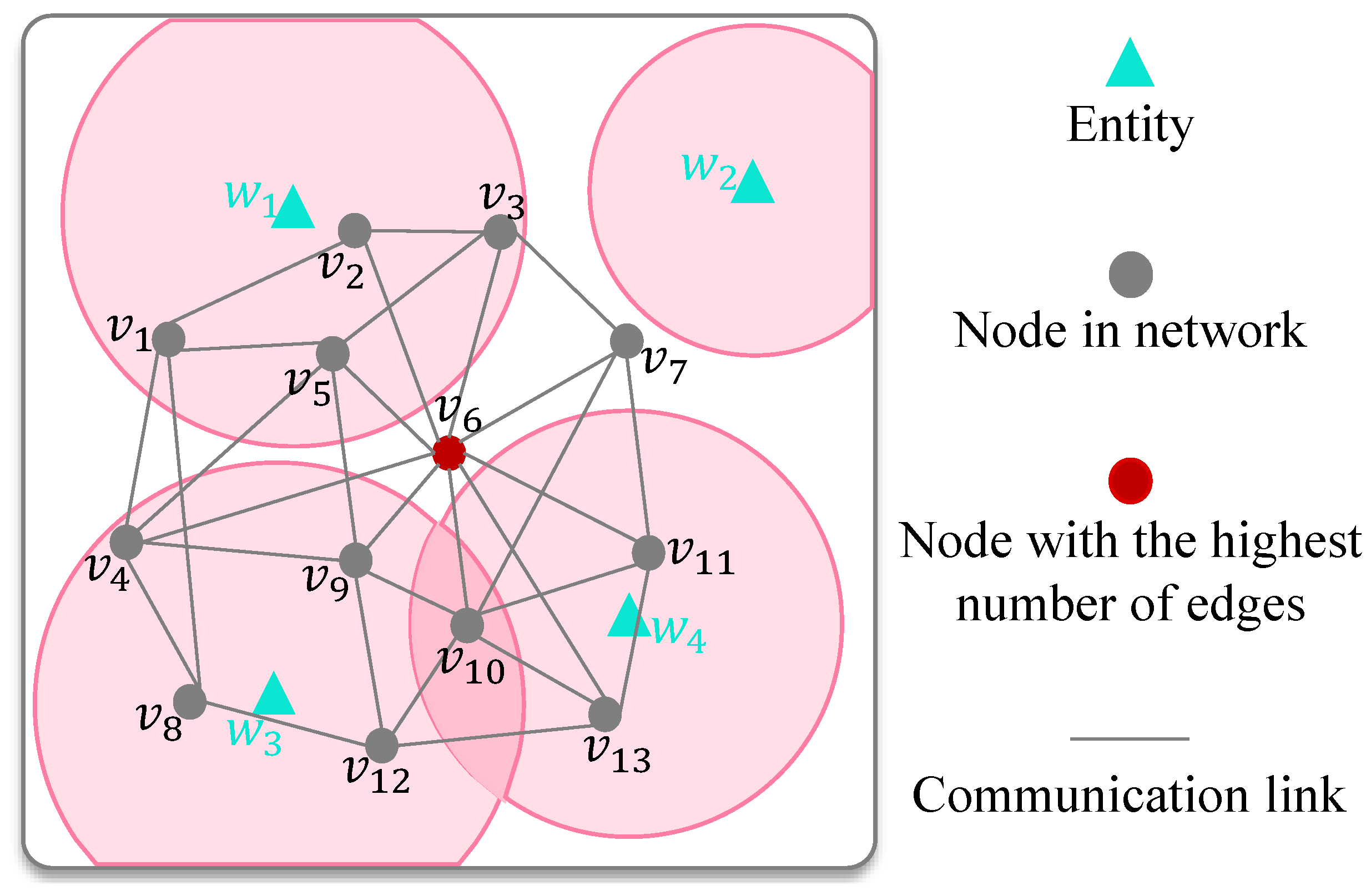
Figure 1 gives an illustrative scenario example of network disintegration with entity allocation. In Figure 1, there are thirteen nodes in the network, and node has the highest degree, which usually means it is a crucial node. The attacker has deployed four entities , and each entity has its attack range represented by a light pink part. It is easy to find that the node cannot be destroyed by the attacker. The above example illustrates that network disintegration should consider not only the network structure itself but also the attack effect of entities. In fact, the removal difficulty of nodes in the network is not equal. For example, removing a hub node may require more entities than the other nodes. In addition, each entity can produce limited damage. We will give an example with some detailed values in Figure 2 to illustrate that the resource allocation strategy has important impacts on network disintegration.
In this paper, we study the problem of optimizing resource allocation to maximize the effect of network disintegration. There are three main challenges in solving the above problem: (i) How can we accurately allocate the limited entities to maximize the disintegration effect? There are many factors in producing the final solution, including the heterogeneity of the removal difficulty of nodes, the attack range of entities, the attack ability values of different entities, and so on. Furthermore, as the entities can only be used in a discretized way, there must exist a resource fragmentation problem. (ii) How can we dynamically generate the disintegration strategy? For example, when destroying terrorist networks, weapon entities and terrorists will dynamically join or exit the war on demand, which makes the designed disintegration strategy variable. It is challenging to generate a disintegration strategy with adaptability. (iii) How can we quickly determine the resource allocation solution in large-scale cases? The network disintegration is an NP-hard problem [16]. Traditional research on network disintegration mainly adopts approximation and metaheuristic algorithms, which often struggle to strike a satisfactory balance between solution speed and quality [17,18,19].The less computer running time it takes to search for a satisfactory solution from many alternative disintegration strategies, the faster it can make decisions and take action, and the greater the opportunity to eliminate terrorist networks and virus networks.
To tackle the above challenges, we propose a deep reinforcement learning-based approach for the network disintegration problem. DRL has achieved a satisfactory balance between effectiveness and efficiency in solving combinatorial optimization problems over the past decade [20,21,22]. To sum up, the main contributions of this paper include the following:
- We model the network disintegration problem with discrete entity allocation using nonlinear optimization programming. By looking into the characteristics of limited entity resources and the heterogeneity of the removal difficulty of different nodes, we reveal that existing solutions cannot balance effectiveness and efficiency well.
- We propose Net-Cracker, a deep reinforcement learning method to solve the network disintegration problem. This approach transforms the two-stage entity and network node selection task in the solution process into a new object selection form so as to simplify the solving process.
- We conduct extensive experiments in multiple settings. The results demonstrate that our method has significant advantages regarding solution quality, computation time and scalability compared to the traditional method.
The rest of the paper is organized as follows. In Section 2, we present the related work on network disintegration and deep reinforcement learning. In Section 3, we give the problem of network disintegration and the mathematical model. Then, we describe the Net-Cracker model in detail in Section 4. Our evaluation method and experimental results are shown in Section 5. In Section 6, we discuss the proposed Net-Cracker method. Finally, this paper is concluded in Section 7.
2. Related Work
2.1. Network Disintegration
As an active topic in the research of complex networks, network disintegration has garnered widespread attention from numerous scholars over the past decade. Different studies use different methods to identify the key node set for specific networks, though the results are mixed.
There are two categories of network disintegration research: One is network disintegration without resource limitations. In this case, many scholars have proposed disintegration strategies based on the special structural properties of nodes, including degree-based strategy [23], betweenness-based strategy [24], and clustering coefficient-based strategy [25], in which the declining order of node properties remove nodes. Furthermore, disintegration methods have been designed based on the structural characteristics of the network. Deng et al. [13] present a multiplex network disintegration strategy based on Tabu search, in which the disintegration effect is superior to typical disintegration strategies. Li et al. [11] put forward an operational capability disintegration method of combat networks under incomplete information. However, network disintegration without resource constraints is often ideal in the real world. For different scenarios, the concretization of resources required to disintegrate a network varies, such as the cost required to eliminate the virus network and the weapon entities required to destroy the terrorist network. Subsequently, another research introduces a network disintegration model with resource limitations [26,27,28], wherein the authors proposed a network disintegration model with limited cost, which assumes that removing different nodes requires different costs. These problems are essentially resource allocation problems [29], that is, how can we allocate cost resources to network nodes so that the disintegration effect is the best.
Nevertheless, a crucial issue is that although existing research incorporates cost resource constraints into network disintegration, this cost is a continuous resource. But empirically, the resources required for some network disintegration are concrete entities, tools or services that have discrete attributes. The current disintegration method cannot solve the network disintegration problem with discrete resources. Furthermore, most existing research focuses on the structural characteristics of networks to design a disintegration strategy, with little consideration of this situation of destroying harmful networks with limited entity resources from an attack view.
2.2. Deep Reinforcement Learning in Combinatorial Optimization Problems
Combinatorial optimization problems (COPs) are widely used in national defense, transportation, product manufacturing and other fields [30]. Common COPs, such as the traveling salesman problem (TSP) [31], vehicle routing problem (VRP) [32], and minimum vertex cover problem (MVC) [33], aim to find the optimal solution from a set of finite objects and are NP-hard. The traditional method for solving COPs mainly adopts exact approaches [34] and approximate approaches [35]. However, as the scale of practical problems and the need for real-time solutions increase, it is difficult for traditional methods to generate optimal COP solutions quickly. Moreover, traditional methods use iterative search and lack the ability to learn from historical data. As soon as the data for the same problem changes, it has to be searched and solved again, resulting in higher computational costs.
To tackle the above issue, the researchers proposed an end-to-end DRL method [36]: the trained deep neural network is used to directly output the solution to the problem, in which the parameters of the neural network are generally trained by a set of problem instances of the same type.
Hopfield et al. [37] first attempted to use neural networks to solve a COP and verified it on a small-scale TSP. However, for a newly given TSP, it has to be trained again from scratch, which has no advantage over the traditional algorithm. To effectively solve COPs, based on the sequence-to-sequence (Seq2Seq) model in the field of machine translation [38], Vinyals et al. [39] proposed a pointer network model for a TSP. It achieved satisfactory results, which triggered a wave of using deep neural networks to solve COPs. Subsequently, to alleviate the challenge of the difficulty in obtaining labels for supervised learning methods, Bello et al. [40] used the reinforcement learning method to train the pointer network model and introduced the critic network as a baseline to reduce the training variance. This approach is more scalable than traditional algorithms on the TSP and KnapSack problem. On the other hand, to solve COPs with graph structure, such as the MVC problem, Dai first proposed a graph neural network named structure2vec to solve COPs [41]. In addition, Li used graph convolutional networks and guided tree search techniques for MVC and maximal independent set (MIS) problems [42]. This approach effectively solves the situation where multiple optimal solutions exist.
2.3. Deep Reinforcement Learning Method in Network Disintegration
DRL has been applied to solve the network disintegration problem because it can effectively find the key node set of the network. Fan et al. proposed a graph neural network (GNN) and DRL to find an optimal set of nodes in networks, which outperformed existing methods in terms of solution quality [43]. Chen et al. also combined DRL and GNN to search high-value edge attack sequences, and proved that the proposed method has strong applicability across various scenarios [44]. Furthermore, various disintegration methods for different networks have also been proposed in current research. Zeng et al. used a combination of graph neural networks and reinforcement learning to address the disintegration problem of heterogeneous combat networks [45]. A DRL algorithm is used to identify the set of key nodes in directed networks [46]. Zeng et al. proposed a solution to the disintegration problem in multiplex networks based on the deep network representation learning model (MINER) [47]. The wide application of the above method shows the potential of using the DRL algorithm to solve network disintegration problems.
3. Network Disintegration Model with Discrete Entity Resources
In this section, we present the mathematical model of network disintegration under the condition that the entity resources are used in a discrete way. For clarity, the main symbols involved in this article are illustrated in Table 1.
3.1. Problem Illustration
As shown in Figure 2, there is a complex network composed of thirteen nodes. The attacker has deployed four entities around the network. Each entity has its attack range, which is illustrated by the light blue circle. It is easy to find that node can be attacked by , can be attacked by , and can be attacked by . Additionally, each entity has different abilities to produce harm, and each node in the network has different removal thresholds. Without loss of generality, the attack abilities of are , respectively. The removal thresholds of are , respectively.
There are different resource allocation strategies to destroy the network. In strategy 1, attacks , attacks , and attacks , which means that can be successfully removed from the network. In strategy 2, attacks and attack , which means that can be successfully removed from the network.
Currently, many researchers have used natural connectivity to measure the effect of network disintegration [27,48], which describes the number of closed loops with different path lengths for all nodes in the network. Let G represent the network topology, and A represent the adjacency matrix of G. The natural connectivity of G, i.e., can be calculated as follows:
in which is the largest eigenvalue of the adjacency matrix .
With Equation (1), we can easily calculate the network connectivity after executing strategy 1 and strategy 2. As shown in Figure 2, the network connectivity in strategy 1 is , while it is in strategy 2.
From the above example, we can formally define the network disintegration problem with discrete entity resources.
Definition 1.
Given a network, which can be represented by , and multiple entities , each node in V has location information and removal threshold, and each entity in W has location information, attack range and attack ability value. Then, the network disintegration problem distributes the entities to proper nodes so that the network connectivity of G is minimized.
3.2. Problem Model
The complex network can be abstracted as an undirected graph, denoted as , where is a node set and is the interactions between nodes. Here, let N and T represent the number of nodes and edges, respectively. The adjacency matrix of G is defined as follows: if and are connected, then ; otherwise, . Furthermore, the node can be described as , where represents the location coordinates of the node , and represents the degree of node , in which the value of is equal to the number of adjacent edges of node .
We assume that the attacker has M entity resources, which can be denoted by a set . The state of the entity can be described by a tuple . Specifically, (i) represents the location coordinates of the entity , (ii) represents the attack ability of the entity, and (iii) indicates the attack range of the entity.
The damaging effect of entities on nodes depends on two aspects: the attack ability value of the entity and the removal threshold of the node. The higher the attack ability value of the entity, the stronger the damage to the node. In addition, the difficulty of removing nodes will escalate as the removal threshold of the node increases. Ren et al. [49] assumed that the cost of removing nodes is proportional to the degree of nodes. Similarly, we define the node removal threshold as the entity attack ability value required to remove the node and assume that is a function of the degree of node , as follows:
where is a random disturbance value, indicating that external factors, such as electromagnetic interference, affect the node removal threshold.
Obviously, only when the node is within the attack range of the entity can the entity be used to attack the node. Here, we use the Euclidean distance to define the distance between the entity and the node , and we use an indicator function to indicate whether can be used to attack , as shown in Equations (3) and (4):
We use the binary variable to determine whether can attack . If attacks , then ; otherwise . To ensure that each entity can only be assigned to attack one node, we have
And to ensure that the entity can only be used to attack nodes within its attack range, we have
The node can be removed only when the damage effects of the entities exceed its removal threshold. In this paper, we assume that the damage effect of multiple entities on the same node is a linear sum of their respective damage values. Let denote the sum of the damage value of the entity to the node , then
We use binary variable to represent whether node can be removed. If node can be removed, then is 1; otherwise, is 0, which can be represented by
Let represent the removed node set, and the network after removing nodes as . Then, the disintegration strategy can be represented by , where if . As introduced in Section 3.1, the effect of the disintegration strategy can be depicted by . The objective of network disintegration is to find a set of disintegration strategies that can minimize the network connectivity.
To sum up, the problem defined in Definition 1 can be represented as follows:
The existing literature [50] has proven that the natural connectivity will strictly decrease once the nodes are removed. Therefore, a lower value implies a more destructive disintegration strategy.
3.3. Complexity Analysis
To prove that the network disintegration problem characterized by Model (9) is NP-hard, we first give the definition of a classic NPC problem, i.e., the subset sum problem [51].
Definition 2.
Given a set of integers , the subset sum problem is to decide whether there exists a subset such that .
Theorem 1.
The network disintegration problem formulated in Model (9) is NP-hard.
Proof of Theorem 1.
Assuming that there is a subset sum instance, e.g., , we could construct an instance of the network disintegration problem from this subset sum problem instance. As shown in Figure 3, there is a network with two crucial nodes . There are also m entities deployed near , and their attack abilities are , respectively. Additionally, we assume that the removal thresholds of both and are . Without loss of generality, we assume that only and lie in the attack range of all entities.
Obviously, if we could optimally solve the network disintegration problem in the constructed example, then we could solve the subset sum problem. If both and are removed, then the answer to the subset problem is “yes”; otherwise, “not”. However, the subset problem is NPC, which shows that the network disintegration problem is also NP-hard. Thus, Theorem 1 is proved. □
4. The Design of Net-Cracker
In this section, we propose an approach named Net-Cracker, which uses the deep reinforcement learning method to find the optimal solution for the network disintegration problem. Firstly, we introduce the framework overview of Net-Cracker, including several key processes. Then, we focus on an encoder–decoder neural network structure with an attention mechanism and explain how Net-Cracker effectively accomplishes the model training.
4.1. Framework Overview
DRL is an agent modeling method that combines the feature extraction capability of deep learning and the sequential decision-making capability of reinforcement learning. For a complex network disintegration problem, we can view it as a Markov Decision Process (MDP) [52]. In each iteration, the agent chooses one object as an action based on the current state and subsequently updates the state. Therefore, solving the network disintegration problem with the DRL method is appropriate. Recent work has shown that AutoML in the field of machine learning lacks transparency and interpretability when dealing with high-risk medical issues [53], which prompted us to opt for an appropriate deep neural network to circumvent these issues. Specifically, in this paper, we primarily employ the actor–critic (AC) method in DRL [54,55]. The AC method entails the actor’s responsibility of generating policies to maximize cumulative returns. Meanwhile, the critic evaluates the policy generated by the actor and provides a value function to guide policy updates. The overall framework of Net-Cracker is shown in Figure 4, and its solving process is divided into three stages: combine, selection, and mapping.
4.1.1. Stage I: Combine
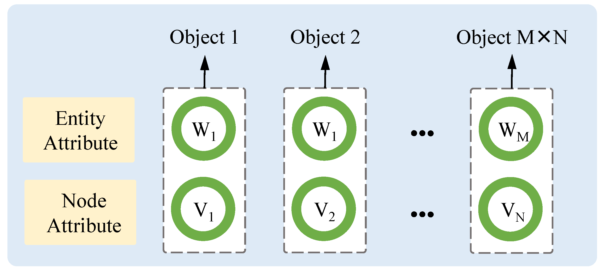
In the combination stage, we combine the current M entities and N nodes distributed on the battlefield through a Cartesian product, resulting in the generation of objects. As shown in Figure 5, each object is the combination of one entity and one node, indicating one selected action candidate. Specifically, the object can be denoted as , which means that the entity i is used to attack the node j.
4.1.2. Stage II: Selection
In the selection stage, we use an encoder–decoder neural network with an attention mechanism to output the optimal solution. Specifically, we initially employ the encoder to extract features from all objects and generate their embeddings (high-dimensional vectors). Subsequently, these embeddings are fed into the decoding neural network for decoding purposes. The decoding process primarily involves selecting an optimal subset of objects from a pool of candidate objects. At each decoding step, we use the decoding neural network in combination with the attention computation method to calculate the attention value of all unselected objects. The agent then greedily selects the object with the highest attention value. Once an object is chosen, it is removed from the candidate object set. This aforementioned decoding process is iteratively repeated until either the maximum constraint on entity attack ability is reached or until the maximum number of steps is exhausted. The structure of the neural network will be illustrated in detail in Section 4.2, and the training process of the neural network parameters will be described in Section 4.3.
4.1.3. Stage III: Mapping
Based on the previous two stages, we can obtain the optimal object set. By mapping the objects into the entity–node pairs, we can derive a selection of entities and removed nodes, subsequently calculating the target value through the objective function .
The design of state, action and reward function is crucial when using reinforcement learning. Specifically, we define the state S as a set of selected objects. At time t, if the agent has already selected objects, then the state information can be expressed as , where . The action space is a set that includes all possible actions that an agent can perform in a specific state. In our problem, selecting an object is considered an action, and thus, the dimension of the action space is . The reward for each solution is defined to be equivalent to its objective function, which measures network performance after nodes are removed.
In this way, we can obtain the solution of the network disintegration problem. During the training phase, we compute the reward value of the solution based on the designed reward function and subsequently employ it for backpropagation and the adjustment of network parameters. Once the loss value of these parameters stabilizes and meets our desired reward criteria, a well-trained network model is obtained. During the testing phase, we can utilize this trained network model to rapidly achieve high-quality disintegration outcomes by inputting entities and nodes in network information.
4.2. Detailed Design of the Neural Network Architecture
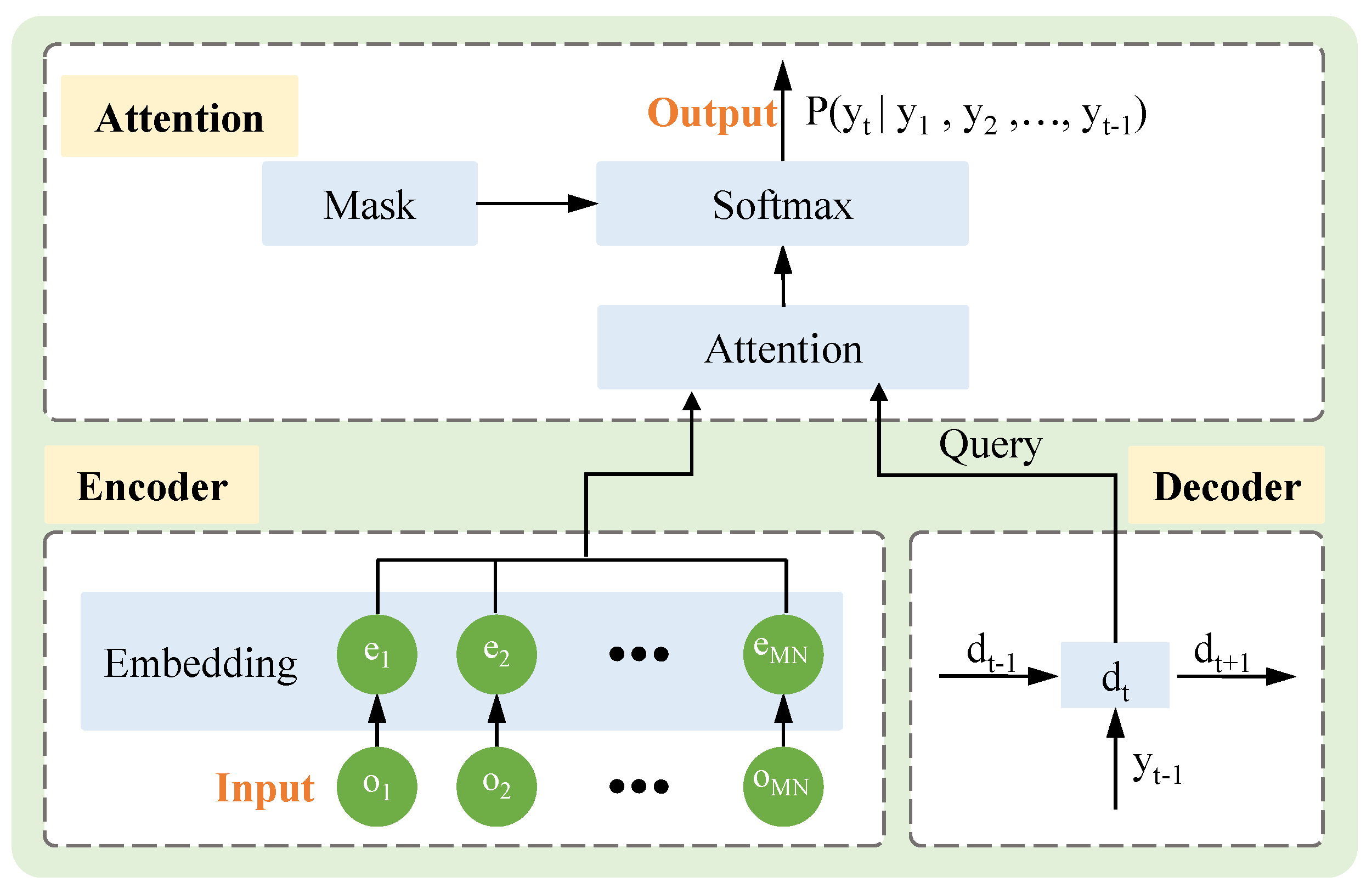
In this section, we mainly introduce the detailed design of the neural network architecture of an actor network in an AC framework that includes encoding, decoding and attention modules, aiming to address the following problems: (i) How can we efficiently extract the multidimensional static information of input objects during the encoding process? (ii) How can we output the probability distribution of selecting each object based on the current state and available action space during the decoding process? (iii) How can we handle the situation where the output objects form an ordered sequence and the length of the output sequence is different from the length of the input sequence? Figure 6 shows the detailed design of the neural network architecture.
4.2.1. The Encoder
The encoder is designed to map the state information of the input sequence, enabling the agent to comprehend the representation of each object. As the order of input object encoding does not affect the choice of subsequent actions, we adopt a one-dimensional convolutional neural network (CNN) as the encoding network to reduce model complexity. Each input object is encoded into an embedding vector , forming an encoding matrix with dimensions , where represents the dimensionality of the target vector.
4.2.2. The Decoder
Using the encoding vector generated by the encoder as input, the decoder sequentially decodes the current state into high-dimensional hidden states. Contrary to the encoding network, the decoding process needs to consider the information of the decoded sequence, so we use the recurrent neural network (RNN) with a memory storage function as the decoding network. In this way, we can obtain the hidden layer state by RNN, where contains the output sequence information of the decoder output before step t and serves as the query for the attention layer.
4.2.3. The Attention
As the output dimension is dynamically determined based on the input vector’s dimension, it is necessary to adjust the dimensions of the output accordingly. The conventional Seq2Seq model lacks flexibility and cannot address this dynamic output dimension problem. Fortunately, Vinyals et al. [39] introduced the attention mechanism into the Seq2Seq model, yielding promising results. Therefore, we also incorporate the attention mechanism into our neural network architecture to tackle this problem. As depicted in Equation (10), at step t, we compute a weighted sum of the decoded hidden layer state and the embedding vector , which is subsequently passed through the tanh activation function.
where v, , and are trainable parameters.
To enhance algorithm efficiency and reduce the action space, we propose incorporating a masking mechanism into the neural network output. For each candidate object, once an object is selected, it will no longer appear in the candidate object set. Specifically, a binary mask is employed to determine the validity of object at time t, as follows:
Finally, we can derive the conditional probability distribution of selecting the next action, which can be represented as follows:
During the training stage, we employ importance sampling to select the next action, ensuring that even actions with low probabilities are considered. However, during the test stage, we adopt the greedy policy to select the action with the highest probability. The detailed solution process of our proposed model is illustrated in Algorithm 1.
| Algorithm 1: Solution Process of the Net-Cracker Model |
 |
4.3. Training Procedure
The AC framework primarily comprises two networks: The actor network, which consists of an encoder, a decoder and an attention module, is designed to generate the probability distribution for action selection in the current state, as previously discussed. On the other hand, the critic network estimates the state value for a given problem instance and shares structural similarities with the encoder of the actor network. During the training process, our main goal is to obtain the optimal network parameters so as to output the best results in the test phase.
For the input problem instance s, the network parameters are set to , and the training objective of the network is defined as follows:
where denotes the objective value of the solution sequence Y under a given instance s.
We use the policy gradient [56] to optimize the following parameters:
where represents the baseline, which is utilized to estimate the expected value of the solution for a given instance and aids in reducing the variance of the gradient.
In practice, problem instances are sampled by the Monte Carlo method, and the average value of these samples is calculated to replace the expected value:
To improve the learning efficiency of actor networks, it is common practice to introduce a parameterized baseline for estimating the expected objective value . Therefore, we introduce a critic network parameterized by to learn the expected objective value found by the current policy given the input instance s. The parameters of the critic network are trained through the mean-squared error between the sampled actual objective value and the estimated value :
where represents the output baseline of the critic.
In our training procedure, the parameters of the critic and actor are updated sequentially simultaneously. The actor parameters are updated by the output of the critic, ensuring that the actor parameters are updated in a positive direction. The detailed training process is depicted in Algorithm 2.
| Algorithm 2: Training Algorithm Based on Actor–Critic. |
 |
5. Performance Evaluation
In this section, we first describe our experimental settings and comparative methods. Then, we present the results of the extensive computational experiment to evaluate the proposed Net-Cracker method.
5.1. Experimental Settings
5.1.1. Dataset
Since the constrained network disintegration problem formulated by Model (9) is being studied for the first time, there are no public datasets. Therefore, we generate the dataset independently as follows.
Two classical synthetic network structures, i.e., scale-free (SF) network and Erdős–Rényi (ER) random network, are selected to construct the architecture of the network. The ER network is a random network, where the connections between nodes follow a Poisson distribution, while the SF network refers to a network in which the node degrees follow a power-law distribution. We set a square area with size to represent the battlefield and then randomly distribute the network nodes and entities on it. The attack ranges of the entities are sampled from a uniform distribution , and the attack abilities of the entities are sampled from a uniform distribution . The value is randomly generated in , which is used to indicate the influence of other factors on the node removal threshold.
We have trained two different Net-Cracker agents and named them DRL-25 and DRL-40, respectively. The DRL-25 model was trained with 10 entities and 15 network nodes, while the DRL-40 model was trained with 15 entities and 25 network nodes. Each model instance was trained using 1 million data points.
5.1.2. Hyperparameter Setting
For each Net-Cracker agent, the encoder of the actor network embeds object information into a 128-dimensional vector by a 1D convolutional network with one layer, while the decoder is a GRU recurrent neural network with 128 hidden units, where Dropout is . The critic network consists of multiple 1D convolutional networks, where the output of the last layer is set to 1. The model uses the Adam optimizer for gradient optimization. The batch size is 128, and the learning rate is .
5.1.3. Device Configuration
We conducted simulation experiments on a computer with the following specifications: CPU: Intel i9-12900K 3.2 GHz; GPU: NVIDIA RTX3090; RAM: 64 GB; OS: 64-bit Ubuntu 16.04. All algorithms are developed using Python 3.7.
5.2. Benchmarks
The network disintegration problem defined in this paper has two decision spaces, i.e., selecting several nodes from the network and assigning appropriate entities to the selected nodes. However, classical disintegration strategies based on node centrality only decide which nodes should be destroyed, but never figure out the resource allocation solution. Therefore, in this paper, we use two classical heuristic algorithms, i.e., genetic algorithms and differential evolution algorithms as the benchmarks.
- Genetic Algorithm (GA): Genetic algorithms search for optimal solutions by simulating the processes of natural selection, inheritance and evolution, and are characterized by simplicity, robustness and strong global search capabilities. By simulating genetic processes such as selection, crossover and mutation, it gradually evolves solutions that better adapt to the given problem. We first encode the entities and nodes in the network, and set the maximum number of iterations, and define the crossover and mutation operations of the GA. Next, we use the natural connectivity of the disintegrated network as the fitness function of the GA for individual evaluation. Finally, the optimal solution to the problem is output based on the fitness function.
- Differential Evolutionary Algorithm (DE): The differential evolution algorithm is an intelligent optimization search algorithm that emerges through cooperation and competition among individuals within a population. It has strengths such as strong adaptability, few control parameters, simple settings and robust optimization results. The solution process of DE is the same as that of GA, but the setting of the mutation scale factor and crossover probability of DE is different from that of GA.
The main parameters of the GA and DE algorithms are depicted in Table 2, where represents the dimension of the decision variables. We set the maximum number of iterations for the GA algorithm to be 200 and 500, denoted as GA-200 and GA-500, respectively. At the same time, the maximum number of iterations for the DE algorithm is set to 200 and 500, referred to as DE-200 and DE-500, respectively.
5.3. Performance Results
In this part, we will demonstrate the performance of Net-Cracker and the benchmarks on solving speed, solving time and generalization ability through the evaluation results.
5.3.1. Solving Quality
To systematically compare the solving quality of the solutions generated by Net-Cracker and other benchmarks, we conducted experiments with different settings on the number of synthesis network nodes from 40 to 160. Ten problem instances are randomly generated, and the average disintegration effect is calculated for each type of network at a given size. The disintegration effect of two synthetic networks is plotted in Figure 7. The smaller the objective value , the better the solution quality of the algorithm.
As shown in Figure 7, the quality of the solutions generated by the Net-Cracker is superior to those generated by the benchmark method in both the ER and SF networks. Specifically, for the ER network, regardless of the size of the problem instance, the average disintegration effect of the DRL-25 algorithm is slightly better than that of the other algorithms. Compared to the heuristic algorithms, the accuracy of the Net-Cracker can be increased by about 8∼10%. For the SF network, when the problem size is 40, 80 and 160, the disintegration performance of DRL-40 is significantly better than GA and DE. At the same time, when the problem size is 120, the solution quality of the DRL-25 algorithm is also superior to GA and DE. The accuracy of the Net-Cracker can be improved by about 50∼62%, indicating that the Net-Cracker is more aggressive in disintegrating the SF network.
5.3.2. Solving Speed
The solution time is crucial for the network disintegration problem. How to quickly generate a disintegration method based on entities and network data is of great significance for seizing the initiative of war. Since the Net-Cracker model used in this paper is end-to-end, only the test time in the application phase is considered when compared with the benchmark algorithm, and the training time is not considered.
We draw the box plots of the solution times of different algorithms when faced with instances of disintegration problems in ER and SF networks, as presented in Figure 8 and Figure 9, respectively. We can see that Net-Cracker can find the solution faster than other benchmark methods, regardless of the problem size of the synthetic network instance. In addition, to further analyze the correlation between the solving speed of the algorithm and the scale of network disintegration problems, we draw a heat map of the average solution time, as shown in Figure 10. As the problem size increases, we can see that the solution time of GA and DE algorithms significantly increases. In particular, GA-500 and DE-500, when dealing with the same problem instances, have significantly better solution quality than GA-200 and DE-200, respectively, but the solution time is more than twice that of GA-200 and DE-200. In contrast, the DRL algorithm can find the solution within 2 s when facing different scale problems, and the solution time fluctuates less.
5.3.3. Generalization Ability
A strong generalization ability enables the model to adapt to new environments, extending beyond its performance on training data alone. During the training phase, we use data with fixed entity capabilities and attack ranges to train the Net-Cracker model. However, in real scenarios, changes in the external environment, such as electromagnetic interference from the enemy and terrain changes, will have an impact on the attack ability and attack range of the entity. When the state of the entity changes, e.g., attack ability and attack range, we need to immediately adjust the resource allocation strategy to maximize the disintegration effect. From the above two subsections of solving speed and solving quality, Net-Cracker can quickly generate high-quality solutions without retraining in the face of problems of different sizes. Next, we will evaluate the performance of the Net-Cracker under changing entity ability and attack ranges.
We also generate problem instances with nodes and then adjust the attack ability and attack range of the entity randomly. It can be seen from Table 3 that the solution quality and speed of Net-Cracker are better than those of the benchmark algorithm on two synthetic networks.
6. Discussion
The Net-Cracker is able to quickly find efficient solutions to address the challenge of low search efficiency faced by traditional methods in eliminating large-scale terrorist networks and blocking the spread of large-scale disease networks. Additionally, because of the powerful generalization ability of the Net-Cracker, even if there are changes in terrorist network members or variations in disease-infected networks, we do not need to spend a lot of time searching for strategies to destroy terrorist networks or block the spread of disease networks. Instead, we can find appropriate solutions quickly. However, there are still several limitations in this study. For example, the types of discrete entity resources used to address network problems are relatively limited. In addition, some complex networks in the real world have heterogeneous edges and nodes and how to reasonably model them is also an important challenge in the future.
7. Conclusions
The disintegration of networks with discrete entity allocations holds significant importance in many areas, for example, eliminating terrorist networks by allocating weapon entity resources, and eliminating disease transmission networks by allocating cabin hospital resources. Figuring out the optimal dissolution solution in many alternative strategies for network disintegration with discrete entity resource allocation is a challenging problem. In this paper, the effect of disintegration is evaluated by the natural connectivity of the network. To maximize this effect, we have designed a DRL-based method, Net-Cracker, which allocates the limited entity resources carefully to achieve the optimization goal. The customized design of Net-Cracker promises that it has good solution quality, solution speed and generalization ability. The results of extensive experiments illustrate that compared with the metaheuristic algorithm, Net-Cracker improves the solution quality by about 8∼62%, while enabling a 30-to-160-fold speed up.
Author Contributions
Conceptualization, R.L. and H.Y.; methodology, R.L., H.Y. and B.R.; software, R.L. and H.Y.; validation, R.L., H.Y. and B.R.; formal analysis, R.L., H.Y., B.R. and X.Z.; investigation, R.L., H.Y., B.R., X.Z., T.C. and X.L.; resources, B.R. and X.Z.; writing—original draft preparation, R.L., H.Y. and X.Z.; writing—review and editing, R.L., H.Y., B.R., X.Z., T.C. and X.L.; supervision, B.R., X.Z., T.C. and X.L.; funding acquisition, B.R. and X.L. All authors have read and agreed to the published version of the manuscript.
Funding
This work was partically supported by the National Natural Science Foundation of China (No. 62302510). The authors would like to thank the support by the COSTA: complex system optimization team of the College of System Engineering at NUDT.
Data Availability Statement
Data will be made available on request.
Conflicts of Interest
The authors declare no conflicts of interest.
References
- Albert, R.; Barabási, A.L. Statistical mechanics of complex networks. Rev. Mod. Phys. 2002, 74, 47. [Google Scholar] [CrossRef]
- Newman, M.E.J. The structure and function of complex networks. Siam Rev. 2003, 45, 167–256. [Google Scholar] [CrossRef]
- Buldyrev, S.V.; Parshani, R.; Paul, G.; Stanley, H.E.; Havlin, S. Catastrophic cascade of failures in interdependent networks. Nature 2010, 464, 1025–1028. [Google Scholar] [CrossRef] [PubMed]
- Wu, J.; Barahona, M.; Tan, Y.J.; Deng, H.Z. Spectral Measure of Structural Robustness in Complex Networks. IEEE Trans. Syst. Man Cybern. Part A 2011, 41, 1244–1252. [Google Scholar] [CrossRef]
- Wu, Z.X.; Holme, P. Onion structure and network robustness. Phys. Rev. E 2011, 84, 026106. [Google Scholar] [CrossRef] [PubMed]
- Arulselvan, A.; Commander, C.W.; Elefteriadou, L.; Pardalos, P.M. Detecting critical nodes in sparse graphs. Comput. Oper. Res. 2009, 36, 2193–2200. [Google Scholar] [CrossRef]
- Raab, J.; ton Milward, H. Dark Networks as Problems. J. Public Adm. Res. Theory J-PART 2003, 13, 413–439. [Google Scholar] [CrossRef]
- Tripathy, R.M.; Bagchi, A.; Mehta, S. A study of rumor control strategies on social networks. In Proceedings of the Acm Conference on Information & Knowledge Management, Toronto, ON, Canada, 26–30 October 2010. [Google Scholar]
- Zdeborová, L.; Zhang, P.; Zhou, H.J. Fast and simple decycling and dismantling of networks. Sci. Rep. 2016, 6, 37954. [Google Scholar] [CrossRef] [PubMed]
- Wandelt, S.; Lin, W.; Sun, X.; Zanin, M. From random failures to targeted attacks in network dismantling. Reliab. Eng. Syst. Saf. 2022, 218, 108146. [Google Scholar] [CrossRef]
- Li, J.; Zhao, D.; Ge, B.; Jiang, J.; Yang, K. Disintegration of Operational Capability of Heterogeneous Combat Networks Under Incomplete Information. IEEE Trans. Syst. Man Cybern. Syst. 2020, 50, 5172–5179. [Google Scholar] [CrossRef]
- Li, Q.; Liu, S.Y.; Yang, X.S. Neighborhood information-based probabilistic algorithm for network disintegration. Expert Syst. Appl. 2020, 139, 112853. [Google Scholar] [CrossRef]
- Deng, Y.; Deng, H.; Wu, J.; Qi, M. Optimal disintegration strategy in multiplex networks. Chaos 2018, 28, 121104. [Google Scholar]
- Wang, T.; Fu, L.; Wei, Z.; Zhou, Y.; Gao, S. Unmanned ground weapon target assignment based on deep Q-learning network with an improved multi-objective artificial bee colony algorithm. Eng. Appl. Artif. Intell. 2023, 117, 105612. [Google Scholar] [CrossRef]
- Quan, L.; Xu, S.; Xu, H.; Chen, F.; Wu, S.; Zhu, J.; Liu, S.; Su, T. Depression, anxiety, lower sleep quality and social support in square cabin hospitals during Shanghai’s COVID-19 lockdown, China. Front. Psychiatry 2024, 15, 1339774. [Google Scholar] [CrossRef]
- Lalou, M.; Tahraoui, M.; Kheddouci, H. The Critical Node Detection Problem in networks: A survey. Comput. Sci. Rev. 2018, 28, 92–117. [Google Scholar] [CrossRef]
- Shen, Y.; Nguyen, N.; Xuan, Y.; Thai, M. On the Discovery of Critical Links and Nodes for Assessing Network Vulnerability. IEEE-Acm Trans. Netw. 2013, 21, 963–973. [Google Scholar] [CrossRef]
- Morone, F.; Makse, H.A. Influence maximization in complex networks through optimal percolation. Nature 2015, 524, 65–68. [Google Scholar] [CrossRef]
- Lozano, M.; Garciá-Martińez, C.; Rodriǵuez, F.; Trujillo, H. Optimizing network attacks by artificial bee colony. Inf. Sci. 2017, 377, 30–50. [Google Scholar] [CrossRef]
- Lin, M.; Chen, T.; Chen, H.; Ren, B.; Zhang, M. When architecture meets AI: A deep reinforcement learning approach for system of systems design. Adv. Eng. Inform. 2023, 56, 101965. [Google Scholar] [CrossRef]
- Wang, Q.; Lai, K.H.; Tang, C. Solving combinatorial optimization problems over graphs with BERT-Based Deep Reinforcement Learning. Inf. Sci. 2023, 619, 930–946. [Google Scholar] [CrossRef]
- Yu, J.J.Q.; Yu, W.; Gu, J. Online Vehicle Routing with Neural Combinatorial Optimization and Deep Reinforcement Learning. IEEE Trans. Intell. Transp. Syst. 2019, 20, 3806–3817. [Google Scholar] [CrossRef]
- Pastor-Satorras, R.; Vespignani, A. Epidemic spreading in scale-free networks. Phys. Rev. Lett. 2000, 86, 3200–3203. [Google Scholar] [CrossRef]
- Borgatti, S.P. Centrality and network flow. Soc. Netw. 2005, 27, 55–71. [Google Scholar] [CrossRef]
- Holme, P.; Kim, B.J.; Yoon, C.N.; Han, S.K. Attack vulnerability of complex networks. Phys. Rev. E 2002, 65, 056109. [Google Scholar] [CrossRef] [PubMed]
- Deng, Y.; Wu, J.; Xiao, Y.; Zhang, M.; Yu, Y.; Zhang, Y. Optimal Disintegration Strategy with Heterogeneous Costs in Complex Networks. IEEE Trans. Syst. Man Cybern. Syst. 2018, 50, 2905–2913. [Google Scholar] [CrossRef]
- Wu, J.; Xiao, Y.; Li, Y.; Deng, Y. Efficient disintegration strategies with cost constraint in complex networks: The crucial role of nodes near average degree. Chaos 2018, 28, 061101. [Google Scholar]
- Li, Q.; Liu, S.; Bai, Y.; He, X.; Yang, X.S. An elitism-based multi-objective evolutionary algorithm for min-cost network disintegration. Knowl.-Based Syst. 2022, 239, 107944. [Google Scholar] [CrossRef]
- Koopman, B.O. The Optimum Distribution of Effort. J. Oper. Res. Soc. Am. 1953, 1, 52–63. [Google Scholar] [CrossRef]
- Papadimitriou, C.H.; Steiglitz, K. Combinatorial Optimization: Algorithms and Complexity; Dover Publications, Inc.: Mineola, NY, USA, 1998. [Google Scholar]
- Dorigo, M.; Gambardella, L. Ant colony system: A cooperative learning approach to the traveling salesman problem. IEEE Trans. Evol. Comput. 1997, 1, 53–66. [Google Scholar] [CrossRef]
- Schulz, A.; Suzuki, Y. An efficient heuristic for the fixed-route vehicle-refueling problem. Transp. Res. Part E Logist. Transp. Rev. 2023, 169, 102963. [Google Scholar] [CrossRef]
- Li, R.; Hu, S.; Zhang, H.; Yin, M. An efficient local search framework for the minimum weighted vertex cover problem. Inf. Sci. 2016, 372, 428–445. [Google Scholar] [CrossRef]
- Marinescu, R.; Dechter, R. AND/OR Branch-and-Bound search for combinatorial optimization in graphical models. Artif. Intell. 2009, 173, 1457–1491. [Google Scholar] [CrossRef]
- Rabiner, L. Combinatorial optimization:Algorithms and complexity. IEEE Trans. Acoust. Speech Signal Process. 2003, 32, 1258–1259. [Google Scholar] [CrossRef]
- Li, K.; Zhang, T.; Wang, R.; Qin, W.; He, H.; Huang, H. Research reviews of combinatorial optimization methods based on deep reinforcement learning. Acta Autom. Sin. 2021, 47, 2521–2537. [Google Scholar]
- Hopfield, J.J.; Tank, D.W. Neural computation of decisions in optimization problems. Biol. Cybern. 1985, 52, 141–152. [Google Scholar] [CrossRef]
- Sutskever, I.; Vinyals, O.; Le, Q.V. Sequence to sequence learning with neural networks. In Proceedings of the NIPS’14: Proceedings of the 27th International Conference on Neural Information Processing Systems, Montreal, QC, Canada, 8–13 December 2014; Volume 2. [Google Scholar]
- Vinyals, O.; Fortunato, M.; Jaitly, N. Pointer Networks. Statistics 2015, 28, 1–9. [Google Scholar]
- Bello, I.; Pham, H.; Le, Q.V.; Norouzi, M.; Bengio, S. Neural Combinatorial Optimization with Reinforcement Learning. arXiv 2016, arXiv:1611.09940. [Google Scholar]
- Dai, H.; Khalil, E.B.; Zhang, Y.; Dilkina, B.; Song, L. Learning Combinatorial Optimization Algorithms over Graphs. Statistics 2017, 30, 1–11. [Google Scholar]
- Li, Z.; Chen, Q.; Koltun, V. Combinatorial optimization with graph convolutional networks and guided tree search. In Proceedings of the NIPS’18: Proceedings of the 32nd International Conference on Neural Information Processing Systems, Montréal, QC, Canada, 3–8 December 2018. [Google Scholar]
- Fan, C.; Sun, Y.; Liu, Y.Y.; Zeng, L. Finding key players in complex networks through deep reinforcement learning. Nat. Mach. Intell. 2020, 2, 317–324. [Google Scholar] [CrossRef]
- Chen, L.; Wang, L.; Zeng, C.; Liu, H.; Chen, J. Searching High-value Edges Attack sequence through deep Reinforcement learning. Knowl.-Based Syst. 2023, 272, 110562. [Google Scholar] [CrossRef]
- Zeng, C.; Liu, H.; Lu, L.; Chen, J.; Zhou, Z. SHATTER: Searching Heterogeneous Combat Network Attack Sequences Through Network Embedding and Reinforcement Learning. IEEE Syst. J. 2023, 17, 4497–4508. [Google Scholar] [CrossRef]
- Yao, W.Z.J. DND: Deep learning-based directed network disintegrator. IEEE J. Emerg. Sel. Top. Circuits Syst. 2023, 13, 841–850. [Google Scholar]
- Zeng, C.; Lu, L.; Liu, H.; Chen, J.; Zhou, Z. Multiplex network disintegration strategy inference based on deep network representation learning. Chaos 2022, 32, 053109. [Google Scholar] [CrossRef] [PubMed]
- Jun, W.; Barahona, M.; Yue-Jin, T.; Hong-Zhong, D. Natural Connectivity of Complex Networks. Chin. Phys. Lett. 2010, 27, 078902. [Google Scholar] [CrossRef]
- Ren, X.L.; Gleinig, N.; Tolić, D.; Antulov-Fantulin, N. Underestimated Cost of Targeted Attacks on Complex Networks. Complexity 2018, 2018, 9826243. [Google Scholar] [CrossRef]
- Yiping, C.; Gerald, P.; Shlomo, H.; Fredrik, L.; H Eugene, S. Finding a better immunization strategy. Phys. Rev. Lett. 2008, 101, 058701. [Google Scholar]
- Schoefield, X.; Tardos, E. Subset Sum Is NP-Complete. 2018. Available online: http://www.cs.cornell.edu/courses/cs4820/2018fa/lectures/subset_sum.pdf (accessed on 3 January 2024).
- Singh, R.; Gupta, A.; Shroff, N.B. Learning in Constrained Markov Decision Processes. IEEE Trans. Control. Netw. Syst. 2023, 10, 441–453. [Google Scholar] [CrossRef]
- Siriborvornratanakul, T. Human behavior in image-based Road Health Inspection Systems despite the emerging AutoML. J. Big Data 2022, 9, 1–17. [Google Scholar] [CrossRef]
- Bahdanau, D.; Brakel, P.; Xu, K.; Goyal, A.; Lowe, R.; Pineau, J.; Courville, A.; Bengio, Y. An actor-critic algorithm for sequence prediction. arXiv 2016, arXiv:1607.07086. [Google Scholar]
- Cheng, Y.; Huang, L.; Chen, C.P.; Wang, X. Robust Actor-Critic with Relative Entropy Regulating Actor. IEEE Trans. Neural Netw. Learn. Syst. 2023, 34, 9054–9063. [Google Scholar] [CrossRef]
- Williams, R.J. Simple statistical gradient-following algorithms for connectionist reinforcement learning. Mach. Learn. 1992, 8, 229–256. [Google Scholar] [CrossRef]
Figure 1.
A simple example to show network disintegration with limited entities.

Figure 2.
Two different disintegration strategies. (a) Three entities attack three network nodes, only two of which can be removed. The network performance after disintegration is 2.12. (b) Three entities attack and remove two network nodes. The network performance after disintegration is 1.77.
Figure 2.
Two different disintegration strategies. (a) Three entities attack three network nodes, only two of which can be removed. The network performance after disintegration is 2.12. (b) Three entities attack and remove two network nodes. The network performance after disintegration is 1.77.

Figure 3.
A simple example to show the network disintegration problem is NP-hard. Only and lie in the attack range of all entities.
Figure 3.
A simple example to show the network disintegration problem is NP-hard. Only and lie in the attack range of all entities.

Figure 4.
The framework of Net-Cracker. In the combination stage, the entity set and node set are combined to form a new object set through the Cartesian product. In the selection stage, we select the object based on the neural network until a complete solution is constructed. The parameters of the neural network can be trained by actor and critic networks. In the mapping phase, by mapping the objects into the entity–node pairs, we can calculate the natural connectivity of the destroyed network.

Figure 5.
Combine entities and nodes into new objects. Each object has the attributes of entities and nodes.
Figure 5.
Combine entities and nodes into new objects. Each object has the attributes of entities and nodes.

Figure 6.
The proposed neural network architecture in AC framework. The encoder extracts the features of the input object through the embedding layer. The decoder is used to store the decoded sequence information. The attention module uses the attention mechanism to output the probability distribution of the following input according to the embedded information and the hidden layer state of the decoding network.

Figure 7.
The average disintegration effect in two synthetic networks by different algorithms.

Figure 8.
The solution time of various algorithms for the ER network disintegration problem at the same scale.
Figure 8.
The solution time of various algorithms for the ER network disintegration problem at the same scale.

Figure 9.
The solution time of various algorithms for the SF network disintegration problem at the same scale.
Figure 9.
The solution time of various algorithms for the SF network disintegration problem at the same scale.


Figure 10.
The correlation between the solving speed of the algorithm and problem scale and the number in each lattice represents the average solution time of the algorithm under a given problem scale.
Figure 10.
The correlation between the solving speed of the algorithm and problem scale and the number in each lattice represents the average solution time of the algorithm under a given problem scale.


Table 1.
Summary of notations.
| Notation | Description |
|---|---|
| G | complex network |
| V | network node set |
| E | network edge set |
| node | |
| edge | |
| the adjacency matrix of G | |
| whether node i is connected with node j | |
| degree of node | |
| W | entity set |
| entity | |
| attack ability of entity | |
| attack range of entity | |
| the removal threshold of node | |
| the distance between entity and node | |
| whether entity attacks node | |
| the sum of damage value to node | |
| whether node can be removed | |
| Y | disintegration strategy |
| the network after removing nodes |
Table 2.
The main parameters of the GA and DE.
| Algorithm | Parameter | Value |
|---|---|---|
| GA | Population size | 100 |
| Maximum number of iterations | 200 and 500 | |
| Selection operator | Tournament selection | |
| Crossover operator | Two-point crossover | |
| Mutation operator | Breeder-GA mutation | |
| Crossover probability | 0.5 | |
| Mutation probability | 1/ | |
| DE | Population size | 100 |
| Maximum number of iterations | 200 and 500 | |
| Crossover probability | 0.5 | |
| Mutation scaling factor | 0.5 |
Table 3.
Comparison of the generalization ability of the algorithm.
| Node Number | GA-200 | GA-500 | DE-200 | DE-500 | DRL-25 | DRL-40 | ||||||
|---|---|---|---|---|---|---|---|---|---|---|---|---|
| Time | Time | Time | Time | Time | Time | |||||||
| ER Network | ||||||||||||
| 40 | 7.84 | 8.05 | 5.30 | 22.32 | 10.54 | 8.41 | 5.94 | 24.06 | 4.09 | 0.31 | 4.33 | 0.30 |
| 80 | 31.41 | 13.21 | 28.97 | 31.91 | 34.07 | 13.97 | 28.83 | 32.60 | 26.75 | 0.61 | 27.40 | 0.59 |
| 120 | 56.24 | 26.30 | 53.81 | 62.17 | 58.77 | 27.38 | 53.97 | 63.06 | 51.61 | 0.87 | 51.73 | 0.94 |
| 160 | 77.20 | 88.89 | 75.10 | 203.67 | 78.61 | 91.10 | 73.33 | 208.94 | 70.22 | 1.18 | 70.26 | 1.21 |
| SF Network | ||||||||||||
| 40 | 1.17 | 7.97 | 0.62 | 19.72 | 2.80 | 8.38 | 0.75 | 20.07 | 0.38 | 0.30 | 0.32 | 0.30 |
| 80 | 3.83 | 13.04 | 3.02 | 32.65 | 5.27 | 13.52 | 3.65 | 31.99 | 1.47 | 0.63 | 1.46 | 0.59 |
| 120 | 5.96 | 24.52 | 5.34 | 60.33 | 6.65 | 25.39 | 5.54 | 61.12 | 2.56 | 0.89 | 4.09 | 0.86 |
| 160 | 5.12 | 84.06 | 3.36 | 191.37 | 6.26 | 87.00 | 3.74 | 193.36 | 1.56 | 1.18 | 1.53 | 1.19 |
Disclaimer/Publisher’s Note: The statements, opinions and data contained in all publications are solely those of the individual author(s) and contributor(s) and not of MDPI and/or the editor(s). MDPI and/or the editor(s) disclaim responsibility for any injury to people or property resulting from any ideas, methods, instructions or products referred to in the content. |
© 2024 by the authors. Licensee MDPI, Basel, Switzerland. This article is an open access article distributed under the terms and conditions of the Creative Commons Attribution (CC BY) license (https://creativecommons.org/licenses/by/4.0/).
Share and Cite
MDPI and ACS Style
Li, R.; Yuan, H.; Ren, B.; Zhang, X.; Chen, T.; Luo, X. When Optimization Meets AI: An Intelligent Approach for Network Disintegration with Discrete Resource Allocation. Mathematics 2024, 12, 1252. https://doi.org/10.3390/math12081252
AMA Style
Li R, Yuan H, Ren B, Zhang X, Chen T, Luo X. When Optimization Meets AI: An Intelligent Approach for Network Disintegration with Discrete Resource Allocation. Mathematics. 2024; 12(8):1252. https://doi.org/10.3390/math12081252
Chicago/Turabian StyleLi, Ruozhe, Hao Yuan, Bangbang Ren, Xiaoxue Zhang, Tao Chen, and Xueshan Luo. 2024. "When Optimization Meets AI: An Intelligent Approach for Network Disintegration with Discrete Resource Allocation" Mathematics 12, no. 8: 1252. https://doi.org/10.3390/math12081252
Note that from the first issue of 2016, this journal uses article numbers instead of page numbers. See further details here.