Variable Neighborhood Search for Multi-Port Berth Allocation with Vessel Speed Optimization

Abstract

This paper delves into the multi-port berth allocation problem (MBAP), enriching the traditional berth allocation problem (BAP) with vessel speed optimization (VSO). In the MBAP, it is assumed that there is cooperation between the port and the shipping companies, and the operation of the vessels and the ports is planned to maximize the overall benefits. Exploring this potential collaboration between ports and shipping entities has the potential to mitigate, or even resolve, the challenges plaguing maritime transportation, e.g., port congestion and suboptimal vessel schedules, to ultimately enhance the efficiency of maritime trade. In this paper, a new mixed-integer linear programming (MILP) model for the MBAP is formulated, which attempts to minimize the total cost incurred during operations, with various constraints such as vessel sailing, the vessel space–time relationship in ports, and the planning period. Meanwhile, an innovative variable neighborhood search (VNS) algorithm is presented, in which the initial solution generation method and neighborhood structures are proposed according to the MBAP characteristics. Furthermore, two sets of MBAP instances are generated to test the proposed MILP and VNS, of which the first set is based on real-world port data and the second on existing studies. The numerical experiments verify that the VNS can efficiently and reliably solve instances of all scales, with each neighborhood structure contributing uniquely to the iterative process. In addition, by analyzing the impact of varying oil prices on the MBAP, the study offers valuable management insights. Finally, a case study based on real data from a port group in the Yangtze River Basin is presented to further demonstrate the necessity of considering vessel service time window and planning period in the MBAP as well as the important role of the VSO in scheduling.

1. Introduction

According to the United Nations Conference on Trade and Development (UNCTAD), shipping and trade patterns have begun to change since 2023, influenced by global trade policy and the geopolitical situation [1]. Meanwhile, the global supply chain crisis has not fully recovered, the maritime market is weak, and the global shipping industry continues to face multiple challenges. As maritime trade began to gradually recover, shipping companies and ports struggle to cope with the surge in throughput. In addition, the UNCTAD has proposed higher standards for the transition to the decarbonization of maritime transportation. Usually, fleet renewal and port expansion are the most straightforward ways to solve shipping dilemmas such as unpunctual vessel schedules and port congestion; however, the high cost is prohibitive. Therefore, the technical improvement in the scheduling level has become the main means to solve these problems.

Port scheduling planning needs to complete the service of arriving vessels, among which the most basic port equipment is berths. Since Lim [2] first defined this problem as the BAP, this problem has been a research hotspot in the past two decades. Early research mainly focuses on the model formulation and algorithm innovation of the discrete and continuous BAP [3,4,5]. Further, more efficient BAP models were developed, such as the multi-objective programming model [6] and bi-layer programming model [7]. According to the reviews on the BAP, Bierwirth and Meisel [8] stated the heuristic algorithm is dominant in solving algorithms [9,10,11]. In addition, Li et al. [12] illustrated that more problem features are considered in the BAP, such as tidal effects [13] and service order [14,15]. Considering environmental sustainability, some scholars have begun to pay attention to emissions during vessel and port operations. Among them, some studies introduce the goal of minimizing carbon emissions in port resource scheduling problems [16,17,18], and some scholars study the promising emissions reduction technology of on-shore power supply [19,20,21,22,23]. In addition, some studies have introduced the VSO into BAP-related problems to reduce emissions during vessel sailing by optimizing vessels’ speeds. Hu [24] studied the relationship between delay times and emissions during vessel sailing and mooring in the BAP, and the experimental results showed that improving the vessel handling efficiency helps to reduce the delay time and emissions. Xia et al. [25] proposed a ship scheduling method with speed reduction to reduce emissions and tested its effectiveness through experiments. Yu et al. [26] proposed a bi-layer multi-objective model by integrating the berth allocation and quay crane assignment problem and vessel speed optimization problem and considering vessel service differentiation. They further developed a nested genetic algorithm, and the experimental results showed that this model can effectively reduce vessel emissions. However, the above studies are still limited to the planning of a single port.

With the evolution of maritime transportation, Venturini et al. [27] realized that independent port scheduling could no longer meet the actual trade demand, and for the first time extended the BAP to multiple ports and introduced the VSO and then proposed the MBAP, which assumes established port–shipping cooperation. Although they proposed a mixed-integer programming (MIP) model for the MBAP, an effective solving method was lacking. Consequently, other scholars further studied the MBAP and proposed the branch-and-cut-and-price algorithm to solve the MBAP [28], a branch-and-cut method [29], and an adaptive large neighborhood search algorithm [30] to solve the MBAP with continuous berth layout.

In summary, research on the MBAP remains limited. Building upon existing MBAP studies [27,28,29,30], this paper formulates a new MILP model that incorporates the vessel space–time relationship constraints proposed by Türkoğulları et al. [31]. Additionally, a VNS algorithm is proposed, tailored to the characteristics of the MBAP through modifications to the initial solution generation method and neighborhood structures. Furthermore, due to the scarcity of publicly available instances, two sets of MBAP instances based on real port data [5] and Agra and Rodrigues [32] are generated. These two sets of instances are used in VNS performance comparison experiments, and some instances in the first set are further applied to oil price sensitivity analysis, yielding management insights based on the results. Finally, an MBAP case study based on real data from a port group is performed and illustrates the importance of enforcing time dimension constraints in scheduling.

In what follows, Section 2 describes the problem characteristics of the MBAP. Section 3 presents the formulated MILP model, while Section 4 elaborates the proposed VNS algorithm. Section 5 showcases all the numerical experiments, and Section 6 provides the conclusion.

2. Problem Statement

The MBAP is an amalgamation of the BAP and the VSO, encompassing berth allocation across multiple ports while considering the speed decisions of vessels between ports. Based on existing studies [27,28], the MBAP assumes that there is cooperation between ports and shipping companies, facilitating information sharing and striving for the maximization of common interests.

Figure 1 illustrates the main components of the MBAP, which comprises vessels and ports. Specifically, adhering to the designated port sequence, vessels sequentially visit ports, completing respective loading and unloading operations. Meanwhile, the port allocates berths for arriving vessels and determines the commencement of work. This process can be regarded as a combination of multiple BAPs, typically depicted using a two-dimensional space–time diagram, as shown in Figure 2. Here, the vertical axis is the time axis, and the horizontal axis is the space axis (the berths of the port). The rectangles symbolize vessels, with their lower end indicating the start time and the upper end representing the departure time. Furthermore, the overlapping rectangle of vessels 4 and 5 in berth 3 illustrates the space–time conflict between vessels.

The relationship among multiple BAPs is established through vessel sailing, and the VSO is further introduced. In the MBAP, the vessel speed is directly related to the fuel consumption and therefore becomes an important part of the total cost. In this paper, the relationship between ship speed and fuel consumption is calculated according to the formula (1) proposed by Venturini et al. [27], where ${\mathcal{l}}_s$ is the vessel fuel consumption per unit distance at the speed $s$, $s^d$ is the designed speed, and $\mathcal{F}$ is the vessel fuel consumption per hour at the design speed.

$${\mathcal{l}}_s=\frac{{\left(\frac{s}{s^d}\right)}^3·\mathcal{F}}{s}$$

(1)

Based on the above description, the MBAP follows the following assumptions.

(a)

The vessel berthing time window is composed of a strict start time window and a soft departure time window; that is, the vessel must start operations after the expected start time but can leave after the expected finish time, the latter of which will incur a delay penalty.

(b)

The potential speed of vessels is discretized over a given range [27].

(c)

Berth depth and width can accommodate all vessels.

(d)

The berthing safety margin is included in all berths.

3. Model Formulation

An MILP model for the MBAP is presented in this section, which is developed from the MIP model proposed by Venturini et al. [27]. In particular, the space–time relationship constraints of vessels are modified according to Türkoğulları et al. [31] and the planning period constraint is introduced.

3.1. Notations

The sets, parameters, and decision variables involved in the proposed MILP model for the MBAP are described in

Table 1. Notations and variables.

Sets and Parameters:
$P$	Set of ports, $P=\{1,\cdots ,|P\left|\right\}$
$B_p$	Set of berths in port $p\in P$, $B_p=\{\mathrm{1,2},\cdots ,|B_p\left|\right\}$
$V$	Set of vessels, $V=\{\mathrm{1,2},\cdots ,|V\left|\right\}$
$S$	Set of speeds, $S$
$P_v$	Port visiting sequence of vessel $v\in V$
$D_{ij}$	Distance between port $i\in P$ and port $j\in P$
${\mathcal{l}}_{vs}$	Fuel consumption per unit of distance for vessel $v\in V$ at speed $s\in S$
$h_{vpb}$	Handling time of vessel $v\in V$ in port $p\in P_v$ at berth $b\in B_p$
${EST}_{vp}$	Expected start time for vessel $v\in V$ in port $p\in P_v$
$EF{T}_{vp}$	Expected finish time for vessel $v\in V$ in port $p\in P_v$
$T$	Planning period
$I$	Unit idle cost caused by vessel waiting.
$E$	Unit delay cost caused by late vessel departure
$O$	Oil price
$H$	Unit handling cost caused by work in port
$M$	Large real number
Decision Variables:
${\mu }_{p{p}^{\prime }}^{vs}$	Binary variable, which equals 1 if vessel $v\in V$ sails from port $p$ to the next port $p^{\prime }$($p,p^{\prime }\in P_v≔p\prec p^{\prime }$) at speed $s\in S$ and 0 otherwise
$a_{vp}$	Arriving time of vessel $v\in V$ in port $p\in P_v$
${\phi }_{vpb}$	Binary variable, which equals 1 if vessel $v\in V$ in port $p\in P_v$ is served at berth $b\in B_v$, and 0 otherwise
$S{T}_{vp}$	Start time of vessel $v\in V$ in port $p\in P_v$
$d_{vp}$	Departure time of vessel $v\in V$ in port $p\in P_v$
$e_{vp}$	Delay time of vessel $v\in V$ in port $p\in P_v$
${\beta }_{ij}^p$	Binary variable, which equals 1 if vessel $j$ starts handling after vessel $i$ ($i,j\in V,i\ne j$) departs in port $p\in P_i\bigcap P_j$ and 0 otherwise.
${\gamma }_{ij}^p$	Binary variable, which equals 1 if vessel $j$ berths at the right berth of vessel $i$ ($i,j\in V,i\ne j$) in port $p\in P_i\bigcap P_j$ and 0 otherwise

.

3.2. Proposed Optimization Model

The MILP model for the MBAP is represented as follows, where $\mathit{Z}$ is the objective value of the problem.

$$\begin{array}{c}\mathrm{M}\mathrm{i}\mathrm{n}\mathit{Z}=\sum _{v\in V}\sum _{p\in P_v}I(S{T}_{vp}-a_{vp})+{\sum }_{v\in V}{\sum }_{p\in P_v}E·e_{vp}+\\ \sum _{v\in V}\sum _{p,p^{\prime }\in P_v\{p\prec p^{\prime }\}}\sum _{s\in S}O\left({\mathcal{l}}_{vs}{D}_{p{p}^{\prime }}{\mu }_{p{p}^{\prime }}^{vs}\right)+\sum _{v\in V}\sum _{p\in P_v}{\sum }_{b\in B_p}H·h_{vpb}·{\phi }_{vpb}\end{array}$$

(2)

s.t.

$$S{T}_{vp}\ge a_{vp},\forall v\in V,p\in P_v$$

(3)

$$S{T}_{vp}\ge {EST}_{vp},\forall v\in V,p\in P_v$$

(4)

$$e_{vp}\ge 0,\forall v\in V,p\in P_v$$

(5)

$$e_{vp}\ge d_{vp}-EF{T}_{vp},\forall v\in V,p\in P_v$$

(6)

$${\sum }_{b\in B_p}{\phi }_{vpb}=1,\forall v\in V,p\in P_v$$

(7)

$$d_{ip}\le {ST}_{jp}+M\left(1-{\beta }_{ij}^p\right),\forall i,j\in V,i\ne j,p\in P_i\bigcap P_j$$

(8)

$${\sum }_{b\in B_p}b·{\phi }_{ipb}+1\le {\sum }_{b\in B_p}b·{\phi }_{jpb}+M\left(1-{\gamma }_{ij}^p\right),\forall i,j\in V,i\ne j,p\in P_i\bigcap P_j$$

(9)

$${\beta }_{ij}^p+{\beta }_{ji}^p+{\gamma }_{ij}^p+{\gamma }_{ji}^p\ge 1,\forall i,j\in V,i\ne j,p\in P_i\bigcap P_j$$

(10)

$$a_{v{p}^{\prime }}=d_{vp}+{\sum }_{s\in S}{\mu }_{p{p}^{\prime }}^{vs}·\frac{D_{p{p}^{\prime }}}{s},\forall v\in V,s\in S,p,p^{\prime }\in P_v\{p\prec p^{\prime }\}$$

(11)

$$d_{vp}=S{T}_{vp}+{\sum }_{b\in B_p}{\phi }_{vpb}·h_{vpb},\forall v\in V,p\in P_v$$

(12)

$$d_{vp}\le T,\forall v\in V,p\in P_v$$

(13)

$${\sum }_{s\in S}{\mu }_{p{p}^{\mathrm{\prime }}}^{vs}=1,\forall v\in V,s\in S,p,p^{\mathrm{\prime }}\in P_v\{p\prec p^{\mathrm{\prime }}\}$$

(14)

$${\mu }_{p{p}^{\mathrm{\prime }}}^{vs}\in \left\{\mathrm{0,1}\right\},\forall v\in V,s\in S,p,p^{\mathrm{\prime }}\in P_v\{p\prec p^{\mathrm{\prime }}\}$$

(15)

$${\phi }_{vpb}\in \left\{\mathrm{0,1}\right\},\forall v\in V,p\in P_v,b\in B_p$$

(16)

$${\beta }_{ij}^p,{\gamma }_{ij}^p\in \left\{\mathrm{0,1}\right\},\forall i,j\in V,i\ne j,p\in P_i\bigcap P_j$$

(17)

$$a_{vp},S{T}_{vp},e_{vp}\ge 0,\forall v\in V,p\in P_v$$

(18)

The objective function (2) attempts to minimize the sum of vessel idle cost, delay cost, sailing cost, and handling cost for all vessels, where “$p,p^{\mathrm{\prime }}\in P_v\{p\prec p^{\mathrm{\prime }}\}$” means vessel $v$ sails to port $p^{\prime }$ after visiting port $p$ [28]. Constraint (3) ensures that the vessel starts working after arrival at the port, and constraint (4) further limits it not earlier than the expected start time. Constraints (5) and (6) determine the delay time of the vessel, which is non-negative. Constraint (7) stipulates that the vessel is berthed in a certain berth in the visiting port. Constraints (8) to (10) prevent conflicts of any two vessels in the same visiting port. Constraints (11) and (12) mandate that a vessel sails to the next visiting port immediately after completing the work. Constraint (13) is the planning time limit, and constraint (14) guarantees that the vessel sails at a certain speed between any two visiting ports. Constraints (15) to (18) set the range of the decision variables.

4. Solution Method

The VNS is a local search meta-heuristic, which was proposed by Mladenović and Hansen [33] and further explained by Hansen and Mladenović [34]. The main ideas of the VNS include shaking and local search (also known as variable neighborhood descent, or VND), and the process is shown as follows.

Step 1: Initialization. Select the set of neighborhood structures ${\mathcal{N}}_k,k=1,\dots ,k_{max}$, to be used in the search; find an initial solution $x$; and set a stopping condition.

Step 2: Set $k\leftarrow 1$.

Step 3: Shaking. Generate a point $x^{\prime }$ at random from the $k^{th}$ neighborhood of $x$ ($x^{\prime }\in {\mathcal{N}}_k\left(x\right))$.

Step 4: Local search. Apply some local search method with $x^{\prime }$ as the initial solution; denote $x^{\prime \prime }$ as the obtained local optimum.

Step 5: Move or not. If this local optimum $x^{\prime \prime }$ is better than the incumbent (currently best known) solution, move to the new optimum ($x\leftarrow x^{\prime \prime }$) and set $k\leftarrow 1$; otherwise, set $k\leftarrow k+1$.

Step 6: If $k\le k_{max}$, skip to Step 3; otherwise, the stopping condition is reached.

In this section, we propose a VNS algorithm tailored specifically for the MBAP. We introduce a set of neighborhood structures designed to suit the unique characteristics of the MBAP, along with an integrated initial solution generation strategy.

4.1. VNS Framework

In the MBAP, the main decision variables of any vessel $v\in V$ in each visiting port $p\in P_v$ include the sailing speed ($s_{vp}$), the work start time ($S{T}_{vp}$), and the choice of berth ($b_{vp}$). The remaining variables can be calculated according to these. Therefore, the main decision variable set $K_{vp}=\{s_{vp},S{T}_{vp},b_{vp}\}$ of vessel $v$ in port $p$ is defined, and the decision information of the solution $x$ of MBAP includes all $K_{vp}$.

Further, Algorithm 1 provides the VNS framework for solving the MBAP. Specifically, based on the given shaking neighborhood structure $N_i^k\left(x\right),i=\{\mathrm{1,2},\dots ,k_{max}\}$, local search neighborhood structure $N_j^l\left(x\right),j=\{\mathrm{1,2},\dots ,l_{max}\}$, and the generated initial solution $x^o$, the VNS starts iterating until it reaches the termination condition (cumulative $I_{max}$ iterations). In each iteration, the incumbent solution $x$ is performed shaking and local search until no better solution is produced. Meanwhile, the local search is repeated whenever a better local solution is found, and the local search for each $N_j^l\left(x\right)$ is performed $t^l$ times.

Algorithm 1 The VNS framework for the MBAP

Input: a set of neighborhood structures $N_i^k\left(x\right),i=\{\mathrm{1,2},\dots ,k_{max}\}$ for shaking, a set of neighborhood structure $N_j^l\left(x\right),j=\{\mathrm{1,2},\dots ,l_{max}\}$ for local search, an initial solution $x^o$.

Set the best solution $x=x^o$.

For $t=1$ to $I_{max}$ do

Set $i=j=1$.

While $i\le k_{max}$ do

Shaking: generate a solution $x^{\prime }$ from $N_i^k\left(x\right)$.

Local search:

While $j\le l_{max}$ do

Find a local best solution $x^{\prime \prime }$ in $t^l$ iterations from $N_j^l\left(x\right)$.

Move or not:

If $\mathit{Z}\left(x^{\prime \prime }\right)<\mathit{Z}\left(x^{\prime }\right)$, then $x^{\prime }=x^{\prime \prime }, j=1$; otherwise $j=j+1$.

End while

Move or not:

If $\mathit{Z}\left(x^{\prime }\right)<\mathit{Z}\left(x\right)$, then $x=x^{\prime }, i=1$; otherwise $i=i+1$.

End while

$t=t+1$.

End for

Output: Best solution $x$.

In the following subsections, the initial solution generation strategy and all neighborhood structures applied in the VNS are further described.

4.2. Initial Solution Generation

The MBAP is complex, and the random initial solution generation method is not only inefficient but also may obtain an infeasible solution. Therefore, a greedy initial solution generation method based on the characteristics of the MBAP is proposed, which is described as follows.

Step 1: Set $p=n=1$.

Step 2: If $n=\left|P\right|+1$, skip to Step 11; otherwise, define set $A_{pn}$, which contains vessels whose $n^{th}$ visiting port is $p$.

Step 3: Randomly select a vessel $v$ in $A_{pn}$.

Step 4: Determine the sailing speed $s_{vp}$ by equation (19), and the arrival time $a_{vp}$ is further calculated by equation (20).

Step 5: Determine the start time $S{T}_{vp}=\max \{a_{vp},ES{T}_{vp}\}$.

Step 6: Define set $\mathit{C}$ according to $S{T}_{vp}$, which contains vessels that conflict with vessel $v$. Also, the berths of non-conflicting vessels are recorded in set $B$.

Step 7: If $B=\varphi$, delay $S{T}_{vp}$ to the earliest departure time of the vessels in $\mathit{C}$, then skip to Step 6; otherwise, determine $b_{vp}$ as the berth with the smallest $h_{vpb}$ in $B$.

Step 8: Based on the final $S{T}_{vp}$, update $s_{vp}$ and $a_{vp}$ by Equations (21) and (20). At this point, the initialization of vessel $v$ is complete, and then $A_{pn}-\left\{v\right\}$.

Step 9: If $p=\left|P\right|$, set $p=1,n=n+1$, and then skip to Step 2.

Step 10: If $A_{pn}=\varphi$, $p=p+1$, then skip to Step 2; otherwise skip to Step 3.

Step 11: Obtain an initial solution for the MBAP.

$$s_{v{p}^{\prime }}=\frac{D_{p{p}^{\prime }} }{{EST}_{v{p}^{\prime }}-d_{vp}},\forall v\in V,p,p^{\prime }\in P_v\{p\prec p^{\prime }\}$$

(19)

$$a_{v{p}^{\prime }}=d_{vp}+\frac{D_{p{p}^{\prime }}}{s_{v{p}^{\prime }}},\forall v\in V,p,p^{\prime }\in P_v\{p\prec p^{\prime }\}$$

(20)

$$s_{v{p}^{\prime }}=\frac{D_{p{p}^{\prime }} }{{ST}_{v{p}^{\prime }}-d_{vp}},\forall v\in V,p,p^{\prime }\in P_v\{p\prec p^{\prime }\}$$

(21)

4.3. Neighborhood Structures

The neighborhood structures of the VNS are mainly applied in shaking and local search steps [34]. The former is mainly used to enrich the diversity of the solutions, while the latter attempts to find local optimal solutions. According to the characteristics of the MBAP and the relationship between decision variables, the following neighborhood structures are proposed in this section.

4.3.1. Shaking

For a given MBAP solution, the shaking step disturbs the speed decision information of some vessels, and the specific neighborhood structure is as follows, where $N_{SK}$ is the number of affected vessels.

Speed Cut: Select $N_{SK}$ vessels with the highest average speed and reduce their maximum speed to the lowest. Higher speed will bring high sailing cost and fuel emissions, which are undesirable. However, blindly reducing the speed may destroy the excellent characteristics of the solution. Therefore, this neighborhood structure considers the average speed but only changes the highest speed among them.

Speed Up: Select $N_{SK}$ vessels with low average speed and increase their minimum speed by one level. Although lower speed is beneficial for cost savings and environmental protection, it can lead to a loss of time. Thus, this neighborhood structure appropriately accelerates vessels with lower average speeds.

Random Speed: Select $N_{SK}$ ships and randomly reset a segment of their speed. This neighborhood structure fully implements randomness and greatly enriches the diversity of solutions.

For vessels whose sailing speed is disturbed, the arrival time is updated according to Equation (20), and the work start time is re-decided according to constraints (3) and (4). However, the above operations may result in conflicts between the affected vessels and other vessels. Taking the disturbed vessel $v^{SK}$ in port $p\in P_{v^{SK}}$ as an example, Figure 3a shows two potential conflict situations, and Figure 3b illustrates the corresponding adjustment methods. Specifically, if vessel $v^{SK}$ conflicts with its predecessor vessel $v^{\mathit{C}}$, the commencement of vessel $v^{SK}$ is delayed until the departure time of vessel $v^{\mathit{C}}$. Otherwise, the vessel $v^{\mathit{C}}$ is adjusted accordingly. After that, the speed and arrival time of the adjusted vessel are updated according to Equations (21) and (20), respectively.

4.3.2. Local Search

For the solutions generated after each shaking, the local search steps are mainly to find better decision information for vessels with different characteristics by applying multiple neighborhood structures. In particular, each neighborhood structure follows the same destroy–repair process as follows, which improves the destroy–repair neighborhood structure proposed by Wagner and Mönch et al. [35].

Step 1: According to the criteria set by the neighborhood structure, select $N_{DR}$ vessels and their decision information will be reset.

Step 2: Destroy. Removes information for $N_{DR}$ vessels from the given solution.

Step 3: Repair. According to Steps 3 to 8 in Section 4.2, re-determine the decision information for these $N_{DR}$ vessels in visiting ports. Taking the decision-making process of a vessel $v\in N_{DR}$ in visiting port $p\in P_v$ with three berths as an example, Figure 4 more intuitively shows the repair process. Specifically, as shown in Figure 4a, under the original $S{T}_{vp}$, vessel $v$ will have conflicts at each berth in port $p$. Since vessel 1 is the first of the potentially conflicting vessels to depart, the $S{T}_{vp}$ is delayed until the departure time of vessel 1. Further, as shown in Figure 4b, the vessel $v$ finds a feasible berth 1.

As can be seen from the above, the difference between the different neighborhood structures lies in the selection criteria for the destroy–repaired vessels, which are described in detail below.

Delay Destroy–Repair: This neighborhood structure removes vessels that have high delay cost. Delays are one of the least desired situations in maritime transportation, and there is a possibility of delays spreading in MBAP [28].

Berth Destroy–Repair: This neighborhood structure considers vessels that have been handling in ports for too long. In addition to the handling time of a vessel in the port being directly related to its own loading and unloading volume, another important factor is the choice of berth. In this paper, the influence of different berths is considered by setting the handling time of different berths, among which the best berth has the shortest handling time. The criterion of this neighborhood structure is based on the relative deviation between the actual handling time and the minimum handling time.

Idle Destroy–Repair: This neighborhood structure gives priority to the selection of vessels with waiting times that are too long. The existence of waiting time for vessels not only generates additional cost but also reflects unreasonable vessel speed optimization.

Random Destroy–Repair: This neighborhood structure is performed at the end of the local search to further enrich the diversity of solutions. Compared with the Random Speed neighborhood structure in the shaking step, this neighborhood structure may apply a better solution.

5. Numerical Results

The VNS algorithm for the MBAP presented above is coded in C++, while the proposed MILP is solved by the commercial solver CPLEX 12.8.0. Since the existing relevant research instances [27,28] cannot be obtained. In this paper, based on the real port data [5] and the instances proposed by Agra and Rodrigues [32], two sets of MBAP instances are generated respectively for numerical experiments. Specifically, each BAP instance proposed by Cordeau et al. [5] and Agra and Rodrigues [32] is taken as the data for a port, and then a complete MBAP instance is generated by combining the data for multiple ports.

The first set of MBAP instances (A1) based on Cordeau et al. [5] is divided into three scales based on the number of vessels and further refined into six categories based on the number of ports. Moreover, the number of port berths and the generation range of distance between ports are also different for each scale instance, as shown in

Table 2. Parameters of the MBAP instances in A1 with different scales.

Instance Scale	Vessel Number	Port Number	Berth Number	Distance
Small (S)	15	{2, 3}	5	[200, 400]
Medium (M)	25	{2, 3}	7	[400, 600]
Large (L)	35	{2, 3}	10	[400, 600]

. In addition, the handling time of vessels at each berth is derived from the Cordeau et al. [5]. Since Cordeau et al. [5] considered the unavailable berths (handling time is 0) that are not considered in this paper, the handling time of these berths in the instances of A1 are the minimum value of the handling time of other berths. Finally, three instances of each type are generated, and each instance in A1 is named according to the format $s\mathit{C}ale\left|P\right|\_\mathcal{k}$, where $s\mathit{C}ale=\{S,M,L\}$, $\left|P\right|$ is the number of vessels, and $\mathcal{k}=\{\mathrm{1,2},3\}$ is the serial number.

The second set of MBAP instances (A2) is based on the instances proposed by Agra and Rodrigues [32], which are derived from Rodrigues and Agra [36] with the number of vessels covered {6, 7, …, 15}. In this section, the instances in A2 consider twice the number of vessels, i.e., the number of vessels covering {12, 14, 16, 18, 20, 22, 24, 26, 28, 30}. The number of ports is set to three in all instances, and the distance between ports is varying in [400, 600]. Other parameters are generated according to the methods proposed by Agra and Rodrigues [32] and Rodrigues and Agra [36]. Specifically, Rodrigues and Agra [36] set the number of berth sections as 34, and the vessel occupancy sections vary in {5, 6, 7}. Based on this, the number of port berths in A2 takes a random value in {5, 6, 7}. Meanwhile, according to the deterministic handling time of vessels proposed by Agra and Rodrigues [32], the disturbance obeying U(1.0, 1.5) is further applied to generate the vessel handling time at each berth in port required in this paper. Finally, the instances in A2 are named R$\left|V\right|$, where $\left|V\right|$ is the number of vessels. More details are available in Agra and Rodrigues [32] and Rodrigues and Agra [36].

For the instances in A1 and A2, the port visiting sequence of each vessel is randomly generated according to the number of ports. Meanwhile, the time window of vessels in each visiting port is generated according to (22) and (23), where s is a random speed and $\zeta$ is the disturbance coefficient following U(−0.3, 0.3). Further, according to Venturini et al. [27], the vessel speed information is discretized into 11 levels with a spacing of 0.5 knots from 14 to 19 knots, and the vessel design speed is set to 19 knots. In addition, the oil price $O$ = USD 250/ton, the idle cost $I$ = USD 200/h, the delay cost $E$ = USD 300/h, the handling cost $H$ = USD 200/h, and the planning period $T$ is set to 1 week.

$$ES{T}_{v{p}^{\prime }}=EF{T}_{vp}+Di{s}_{p{p}^{\prime }}/s,\forall v\in V,s\in S,p,p^{\prime }\in P_v:\{p\prec p^{\prime }\}$$

(22)

$$EF{T}_{vp}=ES{T}_{vp}+\frac{{\sum }_{b\in B_p}{h}_{vpb}}{\left|B_p\right|}(1+\zeta ),\forall v\in V,p\in P_v$$

(23)

Based on the generated MBAP instance sets, the performance comparison experiment for the VNS and CPLEX, the effect test for the VNS neighborhood structures, and the sensitivity analysis for the oil price are performed. All numerical experiments below are performed on a Windows PC with Intel (R) Core (TM) i5-8500 CPU and 8.00 GB RAM. For the VNS, the maximum number of iterations ($I_{max}$) is set to 1000, and the number of iterations for each neighborhood structure in local search ($t^l$) is set to 100. Meanwhile, the number of disturbed vessels in the shaking step ($\left|N_{SK}\right|$) is set to $\left|V\right|/4$, and the number of destroy–repaired vessels in the local search step ($\left|N_{DR}\right|$) is set to $\left|V\right|/2$. Each run records the objective value of the output solution (${\mathit{Z}}^V$) and the solution time. The commercial solver CPLEX limits the maximum solution time to 1 h and records the objective value of the returned solution (${\mathit{Z}}^{\mathit{C}}$), the gap from the optimal solution, and the return time.

5.1. Experimental Comparisons

All the generated MBAP instances are solved by VNS and CPLEX, where the VNS is run 20 times and the objective value of the best solution (${\mathit{Z}}_B^V$), the average objective value (${\mathit{Z}}_A^V$), and the average solution time are recorded. Detailed comparison results are shown in

Table 3. Comparison results of VNS and CPLEX for instances in A1.

Instance	CPLEX			VNS
	${\mathit{Z}}^{\mathit{C}}$	Gap	Time (s)	${\mathit{Z}}_{\mathit{B}}^{\mathit{V}}$	${\mathit{R}}_{\mathit{B}}$	${\mathit{Z}}_{\mathit{A}}^{\mathit{V}}$	${\mathit{R}}_{\mathit{A}}$	Time (s)
S2_01	4.02 × 105	0.00	0.23	4.02 × 105	0.00	4.02 × 105	0.04	5.77
S2_02	4.37 × 105	0.00	0.31	4.37 × 105	0.00	4.37 × 105	0.00	6.53
S2_03	4.87 × 105	0.00	0.27	4.87 × 105	0.00	4.87 × 105	0.00	5.55
M2_01	5.95 × 105	0.15	3600	5.25 × 105	−11.88	5.30 × 105	−10.96	27.31
M2_02	6.35 × 105	0.11	3600	6.03 × 105	−5.12	6.14 × 105	−3.35	25.12
M2_03	6.16 × 105	0.20	3600	5.85 × 105	−5.01	5.92 × 105	−3.79	28.44
L2_01	8.02 × 105	0.35	3600	7.45 × 105	−7.20	7.65 × 105	−4.62	41.17
L2_02	9.65 × 105	0.26	3600	8.74 × 105	−9.42	8.92 × 105	−7.57	47.41
L2_03	8.82 × 105	0.31	3600	7.63 × 105	−13.58	7.78 × 105	−11.80	46.72
S3_01	4.57 × 105	0.00	0.23	4.57 × 105	0.00	4.57 × 105	0.00	6.27
S3_02	5.02 × 105	0.00	0.31	5.02 × 105	0.00	5.03 × 105	0.15	6.85
S3_03	5.24 × 105	0.00	0.27	5.24 × 105	0.00	5.24 × 105	0.00	5.70
M3_01	7.62 × 105	0.32	3600	6.45 × 105	−15.34	6.56 × 105	−13.88	38.20
M3_02	7.08 × 105	0.37	3600	6.11 × 105	−13.70	6.32 × 105	−10.71	35.63
M3_03	7.91 × 105	0.33	3600	7.09 × 105	−10.41	7.28 × 105	−7.98	38.00
L3_01	9.77 × 105	0.47	3600	8.06 × 105	−17.53	8.23 × 105	−15.74	54.96
L3_02	9.83 × 105	0.55	3600	8.33 × 105	−15.32	8.56 × 105	−12.95	53.71
L3_03	1.10 × 106	0.58	3600	8.80 × 105	−20.08	8.89 × 105	−19.33	59.70

and

Table 4. Comparison results of VNS and CPLEX for instances in A2.

Instance	CPLEX			VNS
	${\mathit{Z}}^{\mathit{C}}$	Gap	Time (s)	${\mathit{Z}}_{\mathit{B}}^{\mathit{V}}$	${\mathit{R}}_{\mathit{B}}$	${\mathit{Z}}_{\mathit{A}}^{\mathit{V}}$	${\mathit{R}}_{\mathit{A}}$	Time (s)
R12	3.26 × 105	0.00	0.11	3.26 × 105	0.00	3.26 × 105	0.00	4.74
R14	3.59 × 105	0.00	0.17	3.59 × 105	0.00	3.59 × 105	0.06	5.32
R16	3.46 × 105	0.00	0.15	3.46 × 105	0.00	3.46 × 105	0.02	4.90
R18	4.05 × 105	0.00	215.03	4.05 × 105	0.00	4.06 × 105	0.16	11.22
R20	4.53 × 105	0.00	307.61	4.53 × 105	0.00	4.54 × 105	0.23	18.26
R22	6.34 × 105	0.00	2895.12	6.34 × 105	0.00	6.43 × 105	1.41	29.66
R24	7.96 × 105	0.28	3600	6.96 × 105	−12.63	7.01 × 105	−11.91	34.25
R26	8.44 × 105	0.36	3600	7.45 × 105	−11.65	7.52 × 105	−10.89	40.27
R28	8.91 × 105	0.34	3600	7.66 × 105	−14.00	7.70 × 105	−13.51	38.83
R30	9.58 × 105	0.41	3600	7.96 × 105	−16.92	8.08 × 105	−15.73	43.87

, where the relative deviations ($R_B$ and $R_A$) between the VNS best solution and the average solution and the CPLEX returned solution are, respectively, according to Equation (24).

$$R_i=\frac{{\mathit{Z}}_i^V-{\mathit{Z}}^{\mathit{C}} }{{\mathit{Z}}^{\mathit{C}}}\ast 100\%, i=\{B,A\}$$

(24)

As shown in the results in the A1 instance set in Table 3, for the results of the CPLEX, the optimal solution can be returned within 1 s when solving the small-scale instances, but it cannot be solved within 1 h when the instance scale is enlarged. For the VNS, when solving small-scale instances, the same optimal solution as CPLEX can be obtained within 10 s, but for some small-scale instances (S2_01 and S3_02), the optimal solution cannot be obtained stably. However, the performance advantages of the VNS become obvious in medium- and large-scale instances, where they can not only obtain a better solution than the CPLEX in 1 min but also further improve the stability of the solution. Therefore, the proposed VNS algorithm for solving the MBAP can meet the solving requirements for small-scale instances and has better solving performance than the CPLEX in medium- and large-scale instances.

The results for the A2 instance set shown in Table 4 show the change in solution performance of VNS compared with CPLEX as the number of vessels increases. Specifically, for the R12, R14, and R16 instances, the VNS is able to return the optimal solution (gap is 0) obtained by CPLEX in about 5 s, and the average solution of the 20 runs deviates from the optimal solution by a maximum of 0.06% and a minimum of 0. Further, for the R18, R20, and R22 instances, CPLEX takes a long time to obtain the optimal solution, with a maximum time of 2895.12 s. However, the VNS can still return the optimal solution within 30 s, although the average solution has a maximum relative deviation of 1.41%. As the number of vessels expands further, the advantages of the VNS become significant. For the R26, R28, and R30 instances, the CPLEX can no longer return the optimal solution within 3600 s, while the VNS can obtain a better solution in 1 min, and the average solution is also better than the return solution of the CPLEX. Therefore, the instance set A2 again shows that the proposed VNS can efficiently and stably solve the large-scale MBAP instances.

Further, the effect of the proposed neighborhood structures in the VNS is tested by comparing the change in solution after removing a neighborhood structure. Specifically, first, a neighborhood structure is removed, and then the VNS without it is repeated 20 times to record the best and average solutions and further calculate their relative deviations from the results in Table 3 by Equation (24). The first instance of each medium and large scale in A1 is selected in the experiment. The results are shown in Figure 5 and Figure 6, where each neighborhood structure is represented by its initial letter combination, and “-” means to remove the neighborhood structure.

As shown in Figure 5 and Figure 6, the neighborhood structures applied in shaking and local search play different roles in the VNS optimization process. For the shaking step, the Random Speed (RS) neighborhood structure plays the most significant role, followed by the Speed Cut (SC) and the Speed Up (SU). This is because while most vessels tend to sail at the desired low speed, individual vessels sailing at high speed will bring greater overall benefits. According to the results of local search neighborhood structures, the vessel delay has the greatest influence on the MBAP, followed by vessel waiting and berth selection.

Therefore, in the actual scheduling process, special attention should be paid to those vessels that have delays and exceedingly long wait times. Meanwhile, it is not desirable to blindly reduce the vessel speed only to reduce the fuel consumption, which may bring more serious time costs. Hence, reasonable speed optimization should allow some vessels to sail at higher speeds.

5.2. Sensitivity Analysis of Oil Price

In the MBAP, the oil price determines the vessel sailing cost and is an important factor. This section further explores the impact of oil price on the MBAP through sensitivity analysis, where oil prices are set to USD 250, 400, and 600/ton [27]. The experiment selects the same instances as in Figure 5. Based on the best solution of the VNS runs for 20 times, the average oil consumption and average sailing speed of the vessels are illustrated in Figure 7.

As shown in Figure 7, for all instances, when the oil price increases, the average fuel consumption and average speed of the vessels will decrease. This result suggests that high oil prices will force the vessels to reduce sailing costs by slowing down, even with the potential loss of time. In reality, the oil price is time varying, so it is extremely important to optimize the vessel speed reasonably according to different oil prices. Specifically, when the oil price is high, shipping companies can reduce fuel consumption by appropriate speed reduction but need to consider the minimum time limit in operation. When the oil price is low, it is possible to increase the timeliness of operations by slightly accelerating the vessel speeds to avoid delays.

In general, in the MBAP, the VSO is not only affected by transportation demand but also by time-varying oil prices. Meanwhile, the solution of the VSO is directly related to the berth allocation plan of each port. Therefore, a suitable VSO scheme is flexible and based on demand, port operations, and real-time oil prices.

5.3. An MBAP Case Study

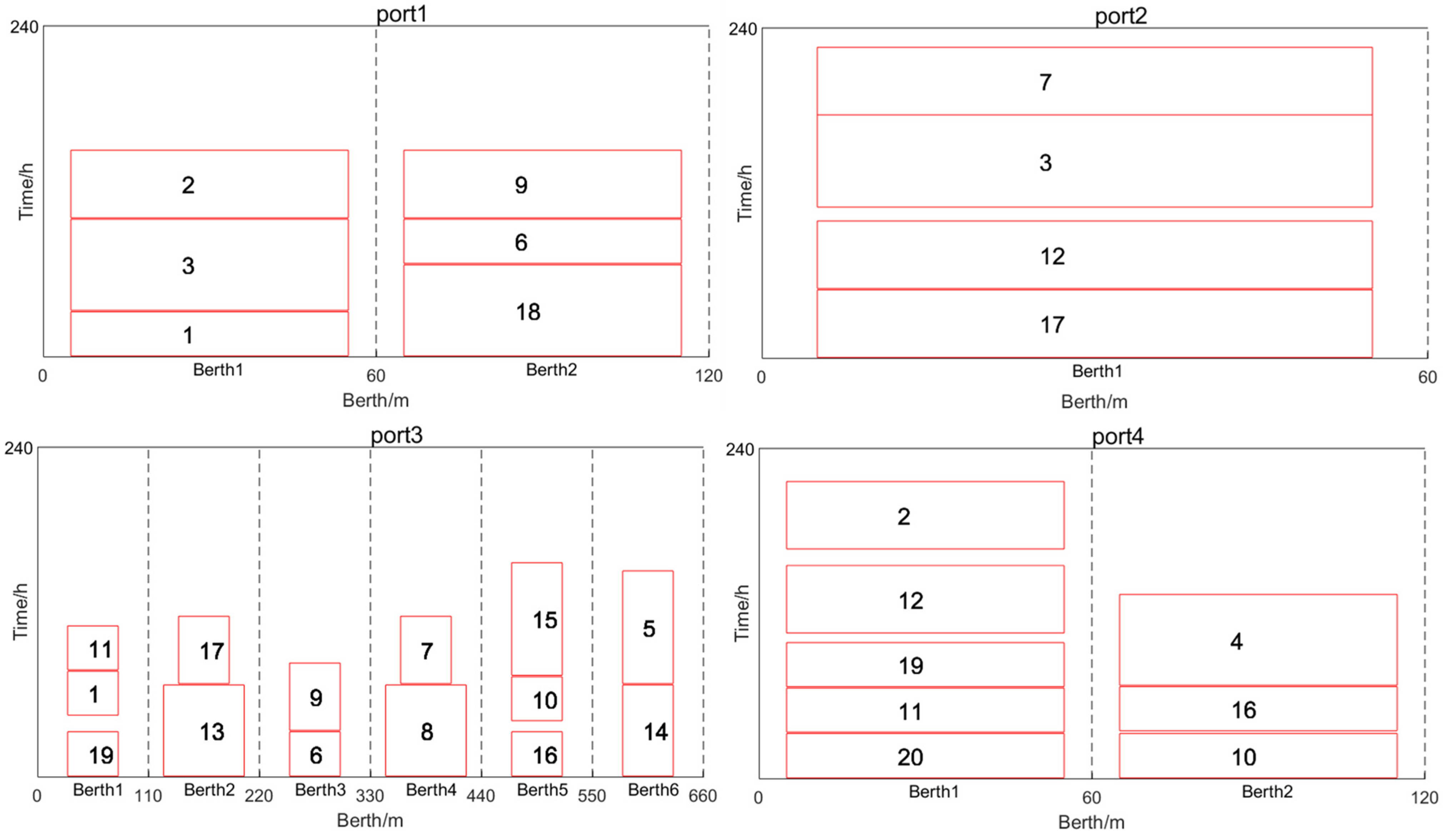
In this section, a case study is conducted based on practical data from a port group in the Yangtze River Basin in central and western China, which is obtained from [37]. This case includes four ports, with the parameters depicted in

Table 5. Port parameters in case study.

Port	Berth Number	Berth Length	Relative Coordinates
Port 1	2	60	(0, 100)
Port 2	1	60	(125, 5)
Port 3	6	110	(195, 35)
Port 4	2	60	(205, 25)

. In order to adapt to the MBAP studied in this paper, the direct linear distance between every two ports is calculated according to the relative coordinates of each port. Meanwhile, the case includes 20 vessels, and the relevant parameters are shown in

Table 6. Vessel parameters in case study.

Vessel	Container Number	Handling Time	Vessel Length	Visiting Sequence
1	100	33	50	1 $\prec$ 3
2	150	50	50	1 $\prec$ 4
3	200	67	50	1 $\prec$ 2
4	200	67	50	4
5	250	83	50	3
6	100	33	50	3 $\prec$ 1
7	150	50	50	3 $\prec$ 2
8	200	67	80	3
9	150	50	50	3 $\prec$ 1
10	100	33	50	4 $\prec$ 3
11	100	33	50	4 $\prec$ 3
12	150	50	50	2 $\prec$ 4
13	200	67	80	3
14	200	67	50	3
15	250	83	50	3
16	100	33	50	3 $\prec$ 4
17	150	50	50	2 $\prec$ 3
18	200	67	50	1
19	100	33	50	3 $\prec$ 4
20	100	33	50	4

. In order to apply the method to the MBAP, the port visiting sequence $P_v$ of each vessel $v$ is randomly generated. Note that due to the limitation of berth length in the original data, ports that could not accommodate vessels are not considered when randomly generating the port visiting sequence for each vessel. The handling time $h_{vpb}$ at each berth in each port is calculated by (25), where ${\mathit{C}}_v$ is the total number of containers (from [37]) and $k^{\mathit{C}}$ is the unit container handling time (set to 20 min according to [37]). In addition, due to the small number of port berths in this case, the planning period has been extended to 10 days, and other parameters are generated in the same way as A1 and A2 instance sets.

$$h_{vpb}={\mathit{C}}_v·\frac{k}{60},\forall v\in V,p\in P_v,b\in B_p$$

(25)

In this MBAP case, the VNS is applied to solve this case 20 times, and the best solution is shown in Figure 8. More specifically, the total cost is USD 753 K, where the sailing cost is USD 19.7 K, the waiting cost is USD 131 K, the handling cost is USD 313 K, and the delay cost is USD 289 K. The average speed of all vessels is 14.92 knots and the total fuel consumption is 78.65 tons, with the latest operational completion time of the vessel 7 being 226 h.

Furthermore, the influence of vessel service time window and planning period on the MBAP is studied. First, the time window restrictions (constraints (4) to (6)) in the proposed MILP model (M0) are removed, and model M1 is obtained as follows:

$$\begin{array}{c}\mathrm{M}\mathrm{i}\mathrm{n}{\mathit{Z}}_1=\sum _{v\in V}\sum _{p\in P_v}I\left(S{T}_{vp}-a_{vp}\right)+\sum _{v\in V}\sum _{p,p^{\prime }\in P_v\{p\prec p^{\prime }\}}\sum _{s\in S}O\left({\mathcal{l}}_{vs}{D}_{p{p}^{\prime }}{\mu }_{p{p}^{\prime }}^{vs}\right)+\\ \sum _{v\in V}\sum _{p\in P_v}{\sum }_{b\in B_p}H·h_{vpb}·{\phi }_{vpb}\end{array}$$

(26)

s.t.

Constraints (3), (7)~(18).

Then, the planning period restriction (constraint (13)) is further relaxed on the basis of M1, and the model M2 is obtained as follows:

$$\mathrm{M}\mathrm{i}\mathrm{n}{\mathit{Z}}_2=\mathrm{M}\mathrm{i}\mathrm{n}{\mathit{Z}}_1$$

(27)

s.t.

Constraints (3), (7)~(12), (14)~(18).

Based on models M1 and M2, the VNS is called for 20 times to solve, and the comparison results between their best solutions and M0 are recorded in

Table 7. Comparison results of different MBAP models.

Model	Average Vessel Speed	Total Fuel Consumption	Latest Completion Time
M0	14.92	78.65	226
M1	14.42	67.21	237
M2	14.00	64.01	273

, including average vessel speed, total fuel consumption, and latest vessel completion time.

As shown in Table 7, the average vessel speed and total fuel consumption decrease when the vessel service time window is removed. Vessels reduce sailing costs by slowing down, since there is no penalty for late departure, and this also leads to an increase in latest vessel completion time. Meanwhile, due to the planning period constraint, the vessels’ deceleration is limited. When the constraint of the planning period is further relaxed, the average vessel speed and total fuel consumption continue to decline, in which the average vessel speed reaches the minimum. At this point, the vessel no longer considers the total completion time, and the latest vessel completion time rises to 273 h. As the constraints of time window and planning period are gradually ignored, the effect of vessel speed optimization gradually disappears, which further leads to a substantial delay in scheduling time. Therefore, it is necessary to integrate vessel speed optimization and consider the vessel service time window and planning period in the MBAP.

In practical scheduling, vessels can be forced to carry out reasonable speed optimization by strictly limiting the planning period and giving delay penalties, which will help alleviate or even solve maritime difficulties such as port congestion and unreliable shipping schedules.

6. Conclusions

This paper investigates the MBAP, offering insights into potential collaborations between ports and shipping companies. Such partnerships aim to enhance maritime transportation efficiency and address existing challenges. Building upon prior research [27,28], we develop a new mixed-integer linear programming (MILP) model for the MBAP, incorporating constraints from Türkoğulları et al. [31] regarding vessel space–time relationships. Additionally, we propose a VNS algorithm to effectively solve the MBAP.

Furthermore, we generated an instance set A1 containing MBAP instances of different sizes using real port data and an MBAP instance set A2 based on BAP instances from existing studies. Numerical experiments performed on the two instance sets demonstrate the efficiency and stability of our proposed VNS algorithm, even for large-scale instances. Moreover, performance tests based on instance set A1 reveal that key factors influencing the MBAP include high-speed sailing, delayed departures, and idle waiting scenarios.

By analyzing the impact of different oil prices on the MBAP, several management insights emerge: (1) Adjusting vessel acceleration can improve the scheduling timeliness during periods of low oil prices. (2) Slowing down during high oil prices can help control overall costs. (3) Shipping companies should consider transportation demand and port operation conditions comprehensively when optimizing vessel speeds. Finally, an MBAP case study demonstrates the importance of integrating VSO in the MBAP as well as the need to consider the vessel service time window and planning period. In conclusion, port-shipping cooperation proves to be an effective strategy for addressing current maritime challenges, with optimized scheduling offering significant benefits to all involved parties. Future research could explore integrating additional port equipment, such as quay cranes, trucks, and yards, into the MBAP for collaborative scheduling. Additionally, considering vessel emissions in ports aligns with the focus on green shipping. Furthermore, given the scarcity of algorithms for solving MBAP-related problems, exploring more efficient solving methods remains a key focus for future research.

References

- United Nations Conference on Trade and Development. Review of Maritime Transport 2023; United Nations Conference on Trade and Development: Geneva, Switzerland, 2023. [Google Scholar]
- Lim, A. The berth planning problem. Oper. Res. Lett. 1998, 22, 105–110. [Google Scholar] [CrossRef]
- Imai, A.; Nishimura, E.; Papadimitriou, S. The dynamic berth allocation problem for a container port. Transp. Res. Part B Methodol. 2001, 35, 401–417. [Google Scholar] [CrossRef]
- Imai, A.; Sun, X.; Nishimura, E.; Papadimitriou, S. Berth allocation in a container port: Using a continuous location space approach. Transp. Res. Part B Methodol. 2005, 39, 199–221. [Google Scholar] [CrossRef]
- Cordeau, J.-F.; Laporte, G.; Legato, P.; Moccia, L. Models and tabu search heuristics for the berth-allocation problem. Transp. Sci. 2005, 39, 526–538. [Google Scholar] [CrossRef]
- Ji, B.; Huang, H.; Samson, S.Y. An enhanced NSGA-II for solving berth allocation and quay crane assignment problem with stochastic arrival times. IEEE Trans. Intell. Transp. Syst. 2022, 24, 459–473. [Google Scholar] [CrossRef]
- Dai, H.; Ma, J.; Yang, Y.; Sun, J.; Dai, Y. A bi-layer model for berth allocation problem based on proactive-reactive strategy. Comput. Ind. Eng. 2023, 179, 109200. [Google Scholar] [CrossRef]
- Bierwirth, C.; Meisel, F. A follow-up survey of berth allocation and quay crane scheduling problems in container terminals. Eur. J. Oper. Res. 2015, 244, 675–689. [Google Scholar] [CrossRef]
- Cheong, C.Y.; Tan, K.C.; Liu, D.K.; Lin, C.J. Multi-objective and prioritized berth allocation in container ports. Ann. Oper. Res. 2010, 180, 63–103. [Google Scholar] [CrossRef]
- Lalla-Ruiz, E.; González-Velarde, J.L.; Melián-Batista, B.; Moreno-Vega, J.M. Biased random key genetic algorithm for the tactical berth allocation problem. Appl. Soft Comput. 2014, 22, 60–76. [Google Scholar] [CrossRef]
- Song, L.; Cherrett, T.; Guan, W. Study on berth planning problem in a container seaport: Using an integrated programming approach. Comput. Ind. Eng. 2012, 62, 119–128. [Google Scholar] [CrossRef]
- Li, B.; Elmi, Z.; Manske, A.; Jacobs, E.; Lau, Y.-Y.; Chen, Q.; A Dulebenets, M. Berth allocation and scheduling at marine container terminals: A state-of-the-art review of solution approaches and relevant scheduling attributes. J. Comput. Des. Eng. 2023, 10, 1707–1735. [Google Scholar] [CrossRef]
- Sheikholeslami, A.; Mardani, M.; Ayazi, E.; Arefkhani, H. A dynamic and discrete berth allocation problem in container terminals considering tide effects. Iran. J. Sci. Technol. Trans. Civ. Eng. 2020, 44, 369–376. [Google Scholar] [CrossRef]
- Yıldırım, M.S.; Aydın, M.M.; Gökkuş, Ü. Simulation optimization of the berth allocation in a container terminal with flexible vessel priority management. Marit. Policy Manag. 2020, 47, 833–848. [Google Scholar] [CrossRef]
- Wu, Y.; Miao, L. An efficient procedure for inserting buffers to generate robust berth plans in container terminals. Discret. Dyn. Nat. Soc. 2021, 2021, 6619538. [Google Scholar] [CrossRef]
- Lin, S.; Zhen, L.; Wang, W.; Tan, Z. Green berth and yard space allocation under carbon tax policy in tidal ports. Marit. Policy Manag. 2023, 50, 1080–1101. [Google Scholar] [CrossRef]
- Wang, T.; Li, M.; Hu, H. Berth allocation and quay crane-yard truck assignment considering carbon emissions in port area. Int. J. Shipp. Transp. Logist. 2019, 11, 216–242. [Google Scholar] [CrossRef]
- Jiang, M.; Ma, F.; Zhang, Y.; Lv, S.; Pei, Z.; Wu, G. Collaborative Scheduling Optimization of Container Port Berths and Cranes under Low-Carbon Environment. Sustainability 2024, 16, 2985. [Google Scholar] [CrossRef]
- Hu, Q.M.; Hu, Z.H.; Du, Y. Berth and quay-crane allocation problem considering fuel consumption and emissions from vessels. Comput. Ind. Eng. 2014, 70, 1–10. [Google Scholar] [CrossRef]
- Peng, Y.; Dong, M.; Li, X.; Liu, H.; Wang, W. Cooperative optimization of shore power allocation and berth allocation: A balance between cost and environmental benefit. J. Clean. Prod. 2021, 279, 123816. [Google Scholar] [CrossRef]
- Zhang, Y.; Liang, C.; Shi, J.; Lim, G.; Wu, Y. Optimal port microgrid scheduling incorporating onshore power supply and berth allocation under uncertainty. Appl. Energy 2022, 313, 118856. [Google Scholar] [CrossRef]
- Yu, J.; Voß, S.; Song, X. Multi-objective optimization of daily use of shore side electricity integrated with quayside operation. J. Clean. Prod. 2022, 351, 131406. [Google Scholar] [CrossRef]
- Yu, J.; Tang, G.; Voß, S.; Song, X. Berth allocation and quay crane assignment considering the adoption of different green technologies. Transp. Res. Part E Logist. Transp. Rev. 2023, 176, 103185. [Google Scholar] [CrossRef]
- Hu, Z.H. Low-emission berth allocation by optimizing sailing speed and mooring time. Transport 2020, 35, 486–499. [Google Scholar] [CrossRef]
- Xia, Z.; Guo, Z.; Wang, W.; Jiang, Y. Joint optimization of ship scheduling and speed reduction: A new strategy considering high transport efficiency and low carbon of ships in port. Ocean Eng. 2021, 233, 109224. [Google Scholar] [CrossRef]
- Yu, J.; Tang, G.; Song, X. Collaboration of vessel speed optimization with berth allocation and quay crane assignment considering vessel service differentiation. Transp. Res. Part E Logist. Transp. Rev. 2022, 160, 102651. [Google Scholar] [CrossRef]
- Venturini, G.; Iris, Ç.; Kontovas, C.A.; Larsen, A. The multi-port berth allocation problem with speed optimization and emission considerations. Transp. Res. Part D Transp. Environ. 2017, 54, 142–159. [Google Scholar] [CrossRef]
- Martin-Iradi, B.; Pacino, D.; Ropke, S. The multiport berth allocation problem with speed optimization: Exact methods and a cooperative game analysis. Transp. Sci. 2022, 56, 972–999. [Google Scholar] [CrossRef]
- Martin-Iradi, B.; Pacino, D.; Ropke, S. The multi-port continuous berth allocation problem with speed optimization. In Proceedings of the International Conference on Computational Logistics, Barcelona, Spain, 21–23 September 2022; Springer International Publishing: Cham, Switzerland, 2022; pp. 31–43. [Google Scholar]
- Martin-Iradi, B.; Pacino, D.; Ropke, S. An adaptive large neighborhood search heuristic for the multi-port continuous berth allocation problem. Eur. J. Oper. Res. 2024, 316, 152–167. [Google Scholar] [CrossRef]
- Türkoğulları, Y.B.; Taşkın, Z.C.; Aras, N.; Altınel, İ.K. Optimal berth allocation and time-invariant quay crane assignment in container terminals. Eur. J. Oper. Res. 2014, 235, 88–101. [Google Scholar] [CrossRef]
- Agra, A.; Rodrigues, F. Distributionally robust optimization for the berth allocation problem under uncertainty. Transp. Res. Part B Methodol. 2022, 164, 1–24. [Google Scholar] [CrossRef]
- Mladenović, N.; Hansen, P. Variable neighborhood search. Comput. Oper. Res. 1997, 24, 1097–1100. [Google Scholar] [CrossRef]
- Hansen, P.; Mladenović, N. Variable neighborhood search: Principles and applications. Eur. J. Oper. Res. 2001, 130, 449–467. [Google Scholar] [CrossRef]
- Wagner, S.; Mönch, L. A variable neighborhood search approach to solve the order batching problem with heterogeneous pick devices. Eur. J. Oper. Res. 2023, 304, 461–475. [Google Scholar] [CrossRef]
- Rodrigues, F.; Agra, A. An exact robust approach for the integrated berth allocation and quay crane scheduling problem under uncertain arrival times. Eur. J. Oper. Res. 2021, 295, 499–516. [Google Scholar] [CrossRef]
- Bi, Y. Multi-port and multi-berth integrated scheduling based on container port cluster. J. Comput. Appl. 2012, 32, 448. [Google Scholar] [CrossRef]
Figure 1.
Diagram of the MBAP.
Figure 2.
Diagram of the BAP.
Figure 3.
Diagram of the vessel conflict adjustment.
Figure 4.
Diagram of the repair process.
Figure 5.
Shaking neighborhood structure effect experiments results.
Figure 6.
Local search neighborhood structure effect experiment results.
Figure 7.
Results of solving MBAP by VNS under different oil prices.
Figure 8.
Diagram of the results of the MBAP case.