
A New Dissimilarity Metric for Anomaly Detection in Management Zones Delineation Constructed from Time-Varying Satellite Images


Department of Computer Science, University of Calgary, Calgary, AB T2N 1N4, Canada
*
Author to whom correspondence should be addressed.
Agriculture 2024, 14(5), 688; https://doi.org/10.3390/agriculture14050688
Submission received: 7 February 2024
/
Revised: 22 April 2024
/
Accepted: 24 April 2024
/
Published: 27 April 2024
(This article belongs to the Topic Geospatial Digital Innovations for Smart Agriculture and Forestry)
Abstract
:A field’s historical performance data are used for management zone delineation in precision agriculture, but including abnormal data leads to inappropriate zones. This paper introduces a framework incorporating historical performance data and a new Zoning Dissimilarity Metric () to detect abnormal zoning data automatically. The methodology identifies abnormal zoning data among the field’s performance indicators extracted from satellite images to enhance the accuracy of the delineated zones. We experimented with our framework using Sentinel-2 images on 39 fields across Canada. Our experimental results, which involve both real and synthetic data, clearly demonstrate the importance of in effectively excluding abnormal data during the zone delineation process.

1. Introduction
Technological advancements have significantly improved the quality and quantity of agricultural products while optimizing costs and minimizing waste and environmental impact. This transformation is crucial due to the increasing global food demand [1]. Precision agriculture leverages sensor data, satellite imagery, and automated systems to monitor critical factors, such as soil health, crop growth, yield parameters, and other related factors, to improve management decisions [2]. However, since factors like soil properties and land topography change from acre to acre, the practice of Delineating Management Zones, or simply zoning, is essential. Zoning divides the field into smaller units for uniform management, allowing for precise farm inputs tailored to each zone [3]. This approach aims to boost profitability while reducing environmental pollution [4,5].
Various methods, including historical soil analysis, yield data, expected yield, and crop coverage, are used to divide farm fields into distinct zones [6], resulting in a zonemap (see Figure 1). Irrespective of the method or data used for zoning, they subdivide a field into units that exhibit varying degrees of performance [7]. A higher level of performance is indicative of increased productivity and crop yield. For example, the field is divided into six management zones in Figure 1. Zone 1 is associated with less performance, and Zone 6 shows the field parts with the best performance.
Due to the non-stationary nature growth conditions, one approach is to average the performance data over multiple years to create a detailed performance map that accurately reflects the varying capabilities of different areas [6]. The challenge with using historical performance data is that certain parts of the field or the whole region may sometimes experience subpar performance due to abnormal natural events, such as severe weather conditions, hail, drought, pests, and other similar factors. These anomalous occurrences can significantly affect the land’s overall performance. Hence, the corresponding data for that specific time may not reflect the normal farming conditions and land potential. Consequently, incorporating such data into the zoning process will result in misleading outcomes and inadequate management zone delineations. In summary, to delineate management zones precisely, evaluating data in advance and excluding those different from normal performance are necessary. This refined approach ensures that the resulting delineated zones better align with the actual capabilities and potentials of the field, offering a more accurate basis for decision-making. This study introduces a framework and a new metric for identifying the abnormal year(s) in the zone delineation process using satellite images.
Historical data from satellite imagery and Normalized Difference Vegetation Index (NDVI) aggregation have been studied to estimate the performance of farm fields [7,8,9], and they have been used in many zoning studies [6]. In our experiments, we generated the performance indicator using historical NDVI data captured on the greenest day of each growing season and named them Peak Green. With one growing season annually, we obtained one peak green image yearly that was used as the growth indicator and included NDVI values at the peak day of each year [10]. To capture abnormal years, we introduced the Zoning Dissimilarity Metric (), which can capture the dissimilarity among peak greens. Using this metric, we could determine the abnormal years in terms of irregular changes in the zonemap.
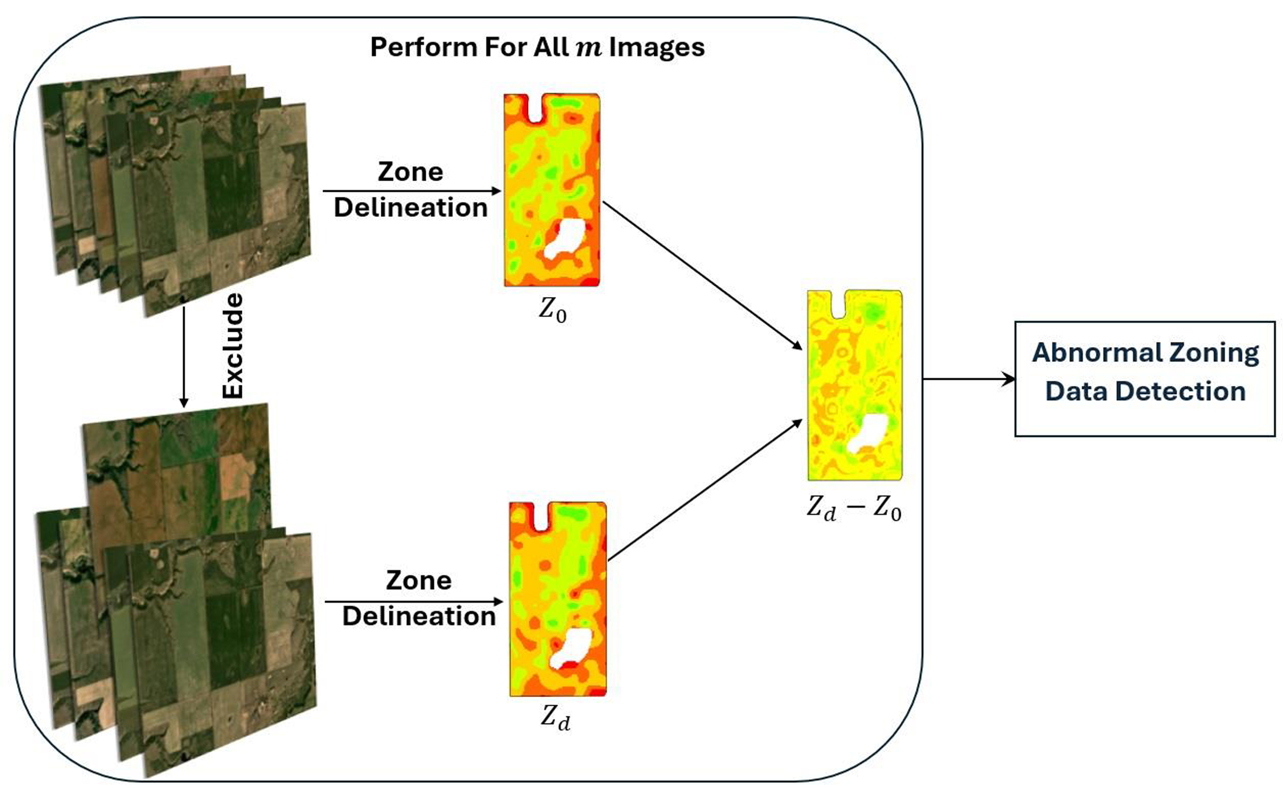
A depiction of the Abnormal Zoning Year(s) Detection Algorithmic Framework is outlined in Figure 2. A set of satellite image data of a field is taken as input for every individual year. In the initial stage of our framework, the zone delineation technique is applied to the input data for all years to obtain the original zonemap. Then, we exclude a test year and re-evaluate the modified or perturbed zonemap. Finally, we measure the change in the resulting zonemaps in two cases by calculating the Zoning Dissimilarity Metric (). Each year’s metric measures how much the zonemap changes by including that specific year’s data in the zoning process. The idea is that the data that abnormally perturb the zonemap correspond to non-normal years. To infer which year is abnormal, we assess the values, and if the relative dispersion of values is higher than a threshold, then the value(s) far away from other values is considered abnormal.
We assessed our methodology in 39 fields and found abnormal years based on their annual data, as discussed in Section 5.1. Furthermore, we evaluated our method by creating synthetically perturbed performance data and precisely identifying anomalous zoning data (Section 5.3). This paper’s main contribution is introducing a new framework and a novel metric for detecting abnormal zoning data using satellite imagery. Identifying and excluding abnormal data enhance the precision of zone labels assigned to each pixel, improving fertility and resource management.
2. Related Works and Background
In this section, we start by discussing variable rate technology usage in precision agriculture. Then, we review studies that use satellite imagery in zone delineation. Finally, anomaly detection in precision agriculture is discussed.
2.1. Variable Rate Technology in Precision Agriculture
A field’s performance varies from acre to acre due to land topography, soil nutrient availability, weather conditions, farm management, and many other factors. While proper nutrition is crucial for optimal plant growth, excessive fertilizer use can lead to environmental pollution and economic losses [11]. Variable rate technology (VRT), or Site-Specific Crop Management (SSCM), is a prominent strategy within precision agriculture that involves adapting resource allocation to account for the variations in soil and crop requirements within the farm field [12]. The management zone delineation technique (zoning) categorizes fields into homogeneous units where each unit is uniformly managed [3].
Zoning enhances decision-making processes regarding efficiently utilizing inputs like fertilizers, agrochemicals, soil ameliorates, pesticides, antiseptics, water, and energy in farm fields [12]. For instance, Khosla and Alley [4] demonstrated how variable rate fertility application reduced fertilizer use in a field with five different zones. They used soil maps from the National Resources Conservation Service for a 36-acre corn field as their input data and showed that fertilizer usage is reduced by about 15% after using this technique.
In conclusion, variable rate technology has been shown to be a promising approach for precision agriculture, where the entire field is divided into manageable homogeneous units, each with specific requirements, allowing for precise resource allocation. Efficient nutrient management enhances crop productivity and promotes environmental sustainability by minimizing excess input use.
2.2. Satellite Imagery in Zoning
Delineating zones is challenging, and many studies have tried to find a reasonable approach to estimate zones [6,13,14,15]. Specifying zones needs detailed datasets for dividing the farm field into distinct regions [7]. Traditionally, soil analysis through physical sampling has been employed to determine the soil class label based on its nutrient composition [16], but it is expensive and time-consuming [12]. In the wake of technological advancements, the utilization of the Internet of Things (IoT), Unmanned Aerial Vehicles (UAVs), and satellite imagery has been increasingly integrated into zone delineation studies [17,18,19]. Notably, remote sensing data, a cost-effective alternative, is increasingly paired with traditional physical soil sampling methods.
In [14], Li et al. used SPOT5 satellite imagery along with Soil Electrical Conductivity (SEC) data as input variables and applied a fuzzy clustering analysis to two principal components. Then, they could group the farm field into three management zones based on the similarity of the soil properties. The study demonstrated that the combination of satellite imagery and soil attributes facilitated the creation of meaningful management zones. Wadoux and Molnar [20] discussed methods for interpreting complex models to classify and predict soil variation. The study revealed that three MODIS satellite imagery covariates, namely MODIS red, green, and SWIR 2 bands, exhibited high importance regarding Soil Organic Carbon (SOC) variation, as indicated by the Random Forest (RF) model analysis.
Researchers have explored the potential of estimating soil organic content solely through remote sensing data. One of the promising approaches is the utilization of vegetation indices that are highly correlated with the health, vigour, and quantity of vegetation [21]. Jin et al. introduced two different methods for estimating Soil Organic Matter Content (SOMC) using spectral bands and showed that some vegetation indices, like the Optimal Difference Index (ODI), the Optimal Ratio Vegetation Index (ORVI), and the Optimal Normalized Difference Vegetation Index (ONDVI), strongly correlate with soil content [22]. Srisomkiew et al. utilized a Data-Driven Soil Assessment (DSA) framework to evaluate soil fertility. They applied a Multiple Linear Regression (MLR) model for soil fertility prediction and showed that soil fertility is correlated with vegetation indices, like the Normalized Difference Water Index (NDWI), the Coloration Index (CL), the Moisture Stress Index (MSI), the and Brightness Index (BI), obtained from the Landsat 8 satellite [23].
Historical satellite images and remote sensing data offer a promising approach to zoning in agriculture. Cammarano et al. [19] leveraged a decade of Landsat data to establish management zones for 540 agricultural fields, concluding that the historical Green Normalized Vegetation Index (GNDVI) serves as a reliable predictor for nitrogen and organic carbon. The NDVI, a widely utilized metric among vegetation indices, has been employed to establish correlations with Soil Organic Matter levels and overall field performance [7,24]. As highlighted in Nawar et al.’s review [6], innovative zoning methods based on satellite imagery data often incorporate the NDVI. Additionally, they demonstrated that the NDVI becomes particularly valuable in cases where yield is not a clear discriminator, aiding in the determination of zone labels. In a complementary approach, Kazemi and Samavati [10] utilized historically normalized NDVI values to generate a fertility map for a field, subsequently using this map to partition the soil into distinct zones. However, challenges such as obtaining cloud-free images persist [25], leading to the exploration of methods like approximating the cloud-covered areas in the images [26] or data averaging [15] to mitigate these limitations.
In conclusion, satellite imagery offers valuable insights into soil fertility and crop coverage, which can be considered field performance data in zoning strategies. Therefore, earth observation satellites are consistent and cost-effective data sources in management zone delineation.
2.3. Anomaly Detection in Zoning
Historical data are not always good representatives of a farm field’s performance. Including abnormal data in decision-making will lead to suboptimal management, increased waste and environmental contamination, and reduced profit. For example, using non-representative performance data in zoning will lead to a suboptimal zonemap.
Efforts to address data quality issues in precision agriculture have led to numerous studies, all with the shared objective of identifying and rectifying data anomalies. For instance, Efrat et al. [27] propose a pipeline to monitor and detect anomalies in dendrometer sensor data. An ensemble of scoring algorithms measure dissimilarity among sensors in an IoT-based system. Moso et al. [28] identify anomalies in crop growth at the harvesting stage based on the dissimilarity of the majority of data points using the Local Outlier Factor (LOF) method. They use GPS datasets from combine machines to detect damaged crops. Catalano et al. [29] introduce a novel machine learning-based approach for anomaly detection in smart agriculture systems, with a primary focus on leveraging multi-sensor systems to monitor sensor health and accurately identify abnormal data patterns. Nevertheless, as highlighted by Schroth et al. [30], identifying non-technical anomalies poses a challenging and unexplored aspect in the realm of data cleansing for precision agriculture. External factors, including natural phenomena such as droughts [31], floods [32], soil erosion [33], pest outbreaks [13], and farmers’ practices [34], can significantly impact crop growth, which can be traced through satellite images.
Abnormal natural event detection has been studied in the literature. For example, using NDVI historical analysis, Rembold et al. [24] indicate drought years. They show that the NDVI is correlated with growing conditions. In drought years, the NDVI value suddenly drops, enabling abnormal growing conditions to be detected. In [32], the NDVI is used to detect floods and the amount of destroyed crops. These events can disrupt zoning data, which are often presumed to represent the field’s actual performance.
While the aforementioned studies contribute to improving data quality in precision agriculture, many approaches lack generalizability in identifying anomalies, making them inapplicable in zoning. Several studies on management zone delineation overlook collective abnormal data detection and elimination before zoning. Instead, the focus is narrowed to addressing noise or statistical outliers in performance data [35].
Most relevant to abnormalities in the zoning process, Ryu et al. [36] studied processes for detecting anomalies in growth conditions in paddy rice fields using vegetation indices. They relied on the phenological characteristics of a specific crop that has a particular sensitivity to stress conditions to distinguish anomalies. While this approach allows for identifying notable deviations from normal growth, it lacks applicability to diverse crop types.
Therefore, adopting a more generalized approach that captures diverse anomalies and operates at the field level using satellite images is essential to recognizing abnormal zoning data. In response to these limitations, our study introduces a method that explicitly targets abnormal data affecting the zoning process after the completion of the growing period. Utilizing satellite-based historical peak green NDVI data as annual performance indicators, our framework employs the Zoning Dissimilarity Metric () to measure abnormality, providing a more generalized and field-specific approach to zoning anomaly detection.
3. Zoning Using Satellite Imagery
In this section, we describe the overview of the chosen zoning technique. Our approach is akin to that in [10] and involved identifying zones based on historical performance. We constructed the performance indicator based on satellite imagery using an algorithm similar to that in [37]. In a high-level overview, our method used Sentinel-2, which has the utmost five-day revisit time, as our satellite imagery resource [38]. We accumulated around 400 to 700 images for each field from 2017 to 2022. The ten-meter-resolution Red and near-infrared (NIR) bands were captured for all available days to calculate the NDVI. Then, peak green was determined independently for each growing season from the cloud-free NDVI images. The resulting peak green images served as the performance indicators and the input data for the zoning process. Other indicators, such as the average of NDVI images, can be used in this approach. The zoning objective is to partition the average of the performance values (i.e., peak green) across all years into k bins, where k represents the number of zones. Using this zoning algorithm, the peak green image is processed and results in the zonemap. All these steps are performed automatically using algorithmic methods. The zoning method is summarized in the following two steps:
- Peak green selection: All cloud-free images are compared with , the maximum pixel-wise peak green for that growing season:where the is calculated usingrepresents an ideal peak green, which is not necessarily achievable by any . However, it helps us to find the peak green image to be selected among images, and it is the one which is the closest to . Therefore, the index p is identified bywhere is the Euclidean distance between and . This estimates the performance of the field.
- Zoning: Selected peak green images are normalized, and their scaled average serves as the input for delineating zones. We expected that the majority of points in the field would exhibit an average performance, and as they deviated from the mean performance value, the number of points was expected to decrease symmetrically. This pattern aligns with the characteristics of a normal distribution. Therefore, we established binning thresholds such that the zones’ areas conformed to a normal distribution. The zoning result is a zonemap assigning labels, from one to k, to each point in the field. The optimum number of zones is studied in [6,39]. Our method is flexible enough to use any zone number (i.e., any k). Figure 3 illustrates two zonemaps automatically created with our method for different zone numbers. Zonemap (a) results from the zoning function when , while zonemap (b) is the output when the zone number is decreased to .
4. Abnormal Zoning Data Detection Method
To ensure the precision of categorizing fields into distinct management zones, it is beneficial to exclude abnormal data. In the following subsections, first, we describe our approach’s principles in Section 4.1 to identify abnormal zoning data. After that, in Section 4.2, the definition of the Zoning Dissimilarity Metric () is explained. Finally, the framework for identifying abnormal zoning data is discussed in Section 4.3.
4.1. An Overview of Our Approach
Our approach’s core principle is to determine abnormal data when that data can largely disturb the zoning result. In our method, we can verify whether including a specific year (or years) can remarkably change the zonemap. The size of the change in the zonemap is the main factor for detecting the abnormality.
To elaborate, we initially set the number of zones, for example, . We let represent the collection of all peak green images we intended to use for zoning. For instance, we could consider as for the first year, as for the second year, and so on. Then, the zoning process was applied on . This process outputs a zonemap, referred to as , as illustrated in Figure 4, left. Modifying by adding or removing some of the images and applying the zoning function to the modified dataset results in , where is the modified dataset (see Figure 4, right). As visualized in the figure, alterations in the input to the zoning process cause shifts in some of the zone labels of pixels.
Zone change arises as the ranking of pixels is altered in the performance data. This means that in scenarios where the entire dataset is uniformly and globally impacted by a factor that does not alter the relative relationships (ranks) between values, the zonemap remains unchanged (see Section 5.4). While techniques such as Spearman Correlation [40,41] can be used to quantify the degree of changes in the ranked datasets, they cannot differentiate between these kinds of global changes (no change in zoning results) versus those changes that disturb the zones. Therefore, another metric that directly measures the zone change is required.
4.2. Dissimilarity Measure Definition
We introduce a new metric for measuring zone changes. This metric aims to capture the change amount in the disturbed zonemap when altering the input dataset. Considering , the created map is chosen as the baseline zonemap. Then, by modifying the performance dataset by adding or removing some images and feeding the new dataset to the zoning process, a new zonemap called is created. Knowing that each zonemap is a matrix of zone labels for the field’s points, and each element in the matrix can be in the range of , the distance of two zonemaps () can be created as a new matrix where each element has a value in the range of . We need to aggregate this distance matrix to one dissimilarity value to enable comparison.
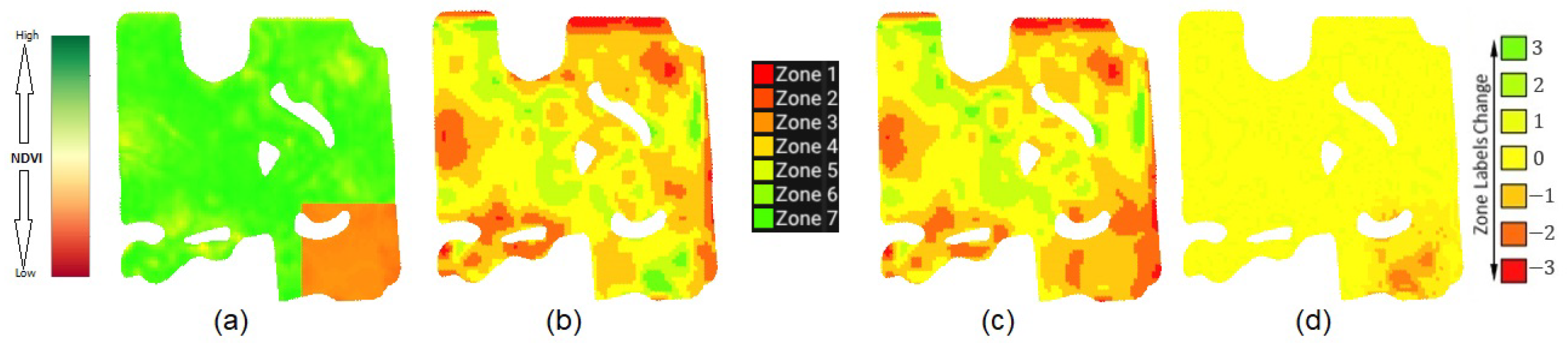
The extent of change is one important factor in computing the dissimilarity value between two zonemaps (i.e., what percentage of the field has a non-zero alternation in the zone label). For instance, in the first row of Table 1, column c depicts a scenario where the change extent is low. Conversely, the row below represents a situation with a change happening in a larger area. However, the extent of change is not enough to measure the difference between two zonemaps; the amount of change per point (pixel) is also important. As illustrated in the row, column d, most pixels changed by one level (green and orange points) and a few pixels changed by two levels (darker orange pixels at the top). However, the changed pixels in column d of the row increased or decreased by just one level.
Another consideration for defining the dissimilarity metric is its independence from the field’s size. It is imperative that we can make comparisons between the zoning effects of one year’s data on two different fields or subfields without the influence of their respective areas. To achieve this, we introduce an area normalization factor in our metric definition, ensuring a fair and unbiased evaluation. Based on these criteria, we define the Zoning Dissimilarity Metric () by
where D denotes all pixels inside of the field and A is the area of D. Notice that when considering the disparity between two matrices comprising integer values (), the negative and positive differences can cancel each other out, which causes a lower that does not properly reflect the changes. Hence, in Equation (4), we calculate the absolute difference. This approach allows us to quantify the amount of change. The denominator is the maximum possible change over all pixels in the field. With this division, we ensure that the field size normalizes the metric. It is worth noting that all out-of-field-boundary pixels are excluded from this calculation (see Figure 5).
values are in , representing the degree of change in zone labels between two zonemaps. A value of zero indicates no change in zone labels, while a value of one signifies that all pixels’ zone labels have changed by the maximum possible amount. For example, in Table 1, one field’s zonemap is created in two cases using its annual performance data from 2017 to 2023. In the first row, column (c), 12% of pixels changed by one level and around 0.2% of pixels changed by two levels. The corresponding is 0.0256 in this case. In the second scenario, the labels of 20% of pixels are all changed by one level, resulting in a of 0.0396. As expected, the second row shows a larger change in that is properly zoning captured with the .
4.3. Abnormal Zoning Year Detection Framework
Based on the defined metric (), we introduce a framework for abnormal zoning year(s) detection, which is depicted in Figure 2. The input data consist of annual performance data. Initially, the is calculated for each year by excluding the data of that specific year. To compute the for the year d () using Equation (4), we use the notation , where . Then, the year(s) with higher values is considered abnormal based on some conditions we will discuss in the following.
We need to establish a threshold for anomaly detection in all fields. Establishing a universal threshold for detecting abnormal zoning data can be challenging and requires careful consideration and analysis. The values for normal years are close to each other and are smaller than 0.02. We did not have enough data for each field. Therefore, we calculated values for all 39 fields in different cases and accumulated approximately 750 measured data points of values. The distribution of these values was revealed to follow a log-normal pattern, as illustrated in Figure 6a. The log-normal distribution is characterized by its right-skewed nature [42], wherein the transformation of values through the natural logarithm yields a normal distribution, , resulting in a dataset with a normal distribution (see Figure 6b).
We employed the one-sigma rule for values to determine an anomaly threshold. Based on the one-sigma rule, approximately 68% of data in a normal distribution fall within one standard deviation from the mean. Because we are not interested in small values that show small change, approximately 16% of the values in a normally distributed dataset may exceed one standard deviation () from the mean. Therefore, based on and we set the threshold at or, simply, . Consequently, values larger than this threshold can be considered abnormal.
Based on our experiments, only relying on the one-sigma rule may result in false-positive anomaly detection, and it may not always be a reliable threshold, as highlighted in previous research [43]. In cases where all values are closely clustered and near the established threshold, there is a risk of misidentifying certain data as abnormal when they are, in fact, too close to each other. Therefore, not all cases that exceed the threshold should be considered abnormal.
The coefficient of variation (CV) is basically normalized to the mean of the data. Higher CV values signify increased data scattering around the mean, implying a higher probability of outliers [44]. We leveraged the CV to add a condition to only investigate anomalies among cases where the standard deviation of values in that field is large relative to the mean.
After calculating the for all years, we obtained an array of values, , where m is the size of the input dataset. Subsequently, the statistical measures, including the mean,
the standard deviation,
and the coefficient of variation
of values are calculated [45]. In instances with very small values, the likelihood of all years’ data being within the normal range is high. Based on the measurement in our dataset, we selected the threshold of 42 for the to filter out data with a small standard deviation relative to the mean.
In summary, abnormality is triggered for year d when the coefficient of variation of the and the value are higher than their thresholds (see Figure 7). This approach allows us to obtain a more farm-adaptive and contextually relevant mechanism for identifying abnormal zoning data.
5. Experiments and Discussion
We first outlined our approach to identifying abnormal years in the experimental fields that experienced drought conditions. Subsequently, we assessed the effectiveness of our method by defining a synthetic year with disturbed performance data and demonstrated how our approach successfully detects this synthetic abnormal data.
The Abnormal Zoning Year Detection Framework is implemented using C++ programming language, and OpenGL is used for visualization purposes. The application (version 1.0) can open the field’s shapefile. Then, the satellite data are downloaded from Sentinel-2. We used Sentinel-Hub API in this regard [10]. After that, the annual performance data are calculated, and zones are delineated automatically based on our zoning algorithm. Finally, the abnormal zoning data are identified. The user can exclude the abnormal zoning data from the dataset (with a simple click on the application), calculate the , and monitor the changes in the new zonemap.
5.1. Experiment on Real Data
Our study areas were 39 selected fields from Canada, mainly in Alberta and Saskatchewan, and encompassed over 9000 acres. They experience a single growing season annually, resulting in only one peak green each year. In this study, we focused on six fields from the larger selection to provide detailed specifications. These fields are provided in Table 2. The table contains the fields’ ID, their boundary shape, the longitude and latitude of two points forming the bounding box of each field, the province where the fields are situated, and the area. The map in Figure 8 displays the spatial distribution of all 39 selected fields.
The results of the for the specified fields are presented in Table 3, and the same results for other fields are presented in Appendix A. The table shows the field ID in the first column and the for each field from 2017 to 2022 in subsequent columns. The mean, standard deviation, and coefficient of variation are presented in the next columns (, , and ). The last column (AZY) indicates the Abnormal Zoning Year for each farm field.
Our method for identifying abnormal zoning data was applied to 39 fields, revealing that in 22 of these fields, the performance data for 2021 were identified as abnormal zoning data that should be excluded from the zoning process. The year 2021 was characterized by widespread drought conditions across many farm fields in Canada, as illustrated in data from [46], shown in Figure 9, where a comparison with a non-drought year is depicted for July. The visual representation clearly shows that many fields experienced severe and extreme drought conditions. Consequently, a strong argument is made for excluding this year’s data in the zoning process for many fields.
Figure 10 visually represents the values for all fields under experimentation for two consecutive years. As depicted on the left side of the figure, during the drought year of 2021, values for 87% of the fields surpass the mean. Conversely, on the right side of the figure, illustrating a normal year, 75% of the fields exhibit values below the mean.
5.2. Discussion
Our experiment demonstrated the effectiveness of the in detecting data that significantly alter the zoning process. For instance, in Table 3, while a substantial value is observed for field number six in the year 2021 (0.1143), other fields exhibit comparatively smaller values for the same year. This suggests that the year 2021 was potentially an abnormal zoning year for field six. However, for field one, the year 2020 had a value that is near the abnormality threshold; the likelihood of abnormality for this year is lower. Furthermore, the for field number five falls below the threshold, indicating that no abnormal years were detected in this field due to the proximity of the values. These findings underscore the heterogeneity of field conditions and the importance of field-specific analyses. By systematically identifying and excluding abnormal years from the zoning process, our method enables a refined analysis of new, smaller datasets.
In our experiments, despite nearly all fields belonging to the drought map in 2021, we found that this year was not identified as abnormal zoning in 17 fields. The scale of the drought map is large and not accurate enough at the level of farm fields. Furthermore, proactive farm management measures can effectively mitigate the impact of abnormal events on a field’s performance. This aligns with the findings from Solh et al. [47], emphasizing the importance of precise management practices like irrigation in reducing drought impacts. Our observations further support this notion, as certain fields facing drought conditions managed to alleviate stress through adept farm management, thus preventing their corresponding performance data from being flagged as abnormal in zoning. This highlights the adaptability of our method to small-scale fields, enabling tailored, field-specific analyses. As a result, the application of large-scale drought maps [46], which are typically used to exclude all corresponding data in the drought region from the zoning process, could benefit from the refinement offered by our method.
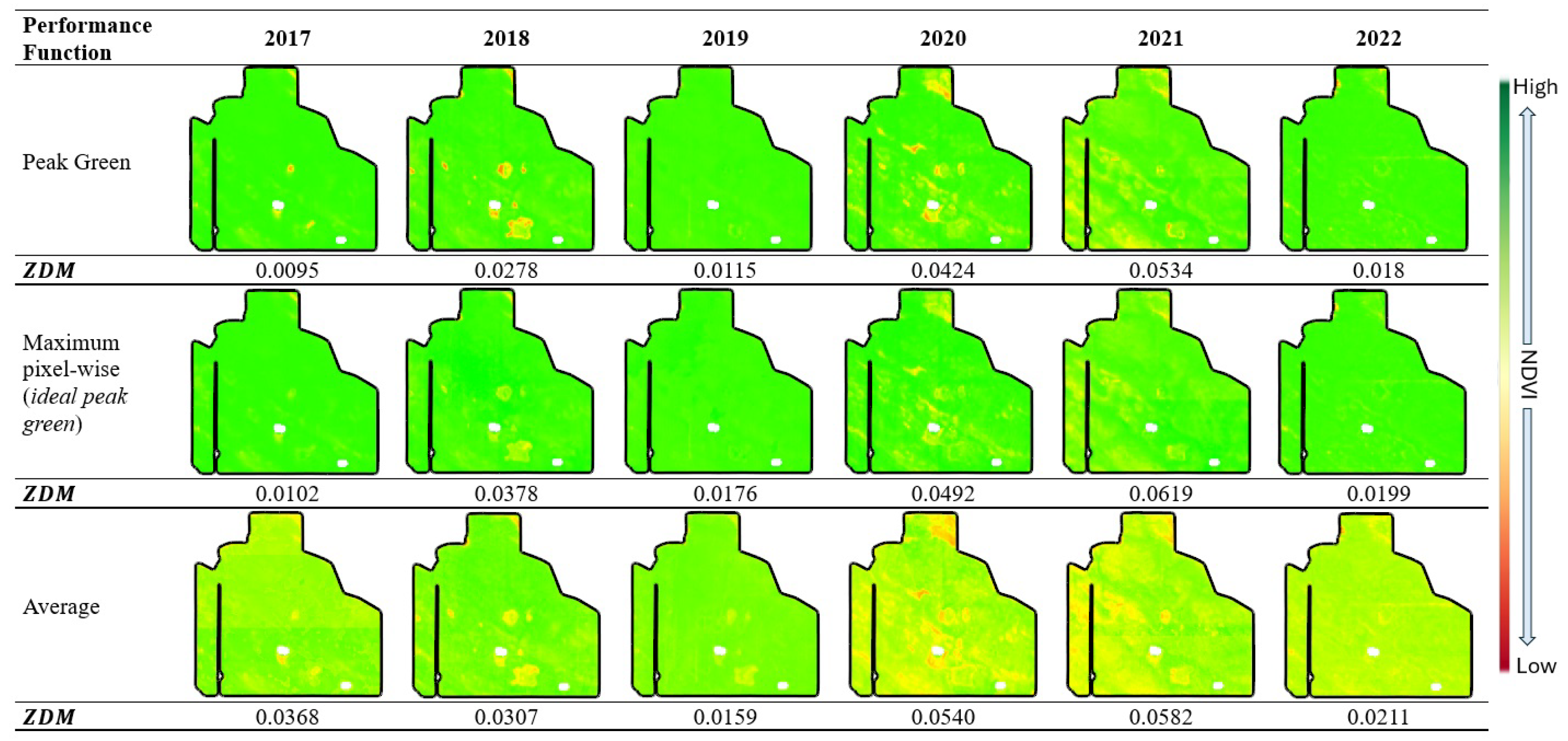
Moreover, our framework demonstrates versatility in its compatibility with various performance functions. While studies such as [10,37] utilized performance metrics like peak green or maximum pixel-wise NDVI to capture maximum productivity potential, these metrics may not fully encompass vegetation dynamics throughout the growing season. Additionally, relying solely on one satellite image exposes the analysis to vulnerability from environmental factors such as precipitation and cloud cover during peak growth times. In contrast, alternative metrics, such as the average NDVI throughout the growing season, as explored in [15,48], offer a more comprehensive view and are less susceptible to the influence of specific weather events or short-term environmental variability but may lack sensitivity to peak performance. Notably, our framework offers the flexibility to seamlessly substitute any of these performance functions with the peak green method.
In one of our experimental fields, we explored the use of both average NDVI and maximum pixel-wise NDVI as alternatives for peak green in our defined zoning function (Section 3). We utilized NDVI images captured from June to the end of October, filtering the data to include only values where . This selection criteria ensured that only meaningful vegetation data during the growing season were considered. Subsequently, the calculated average or maximum pixel-wise NDVI values were integrated into our zoning function. The resulting values for this field are illustrated in Figure 11.
The average NDVI image exhibits lower values compared to the peak green, as depicted in Figure 11. Interestingly, for the years 2019 and 2022, the values show greater similarity, and the years 2020 and 2021 display higher values across the three methods. Although there exists overall consistency among the approaches, these findings suggest that the distribution of values may vary depending on the applied performance function. Consequently, the thresholds should be refined using a similar method as described.
Zoning aims to capture productivity and a field’s performance, making the peak green function particularly pertinent, especially for crops with shorter peak durations. However, the effectiveness of this function may be compromised if cloud-free images during the peak growth period are unavailable. This underscores the importance of carefully selecting performance indicators based on factors such as the crop’s phenology, image temporal resolution, and environmental conditions.
5.3. Experiment on Synthesized Data
We lacked access to the actual performance data for the fields across various years. To validate the accuracy of our identification of abnormal zoning years, we opted to assess the framework using synthetic data. This technique generates a synthetic abnormal year by perturbing the zoning invariant data, (i.e., synthetic data in which the zone labels remain unchanged by including those data). Creating the zoning invariant data is an intermediate state because the value for the unperturbed invariant data is zero. As a result, any impact on the score of perturbed invariant data comes purely from our synthetic perturbation. To create zoning invariant data using , the relative rank of pixels in the field should be the same as averaged performance data over the years. In this way, the resulting zonemap remains unchanged. Therefore, using the averaged performance, we can create . By deliberately perturbing , we create abnormal synthetic data. Then, we can verify our abnormal detection framework.
The inspiration for this evaluation type stems from the possibility of partial damage occurring in the field due to severe weather conditions, such as hail damage, affecting only a portion of the area. To explore this concept, in the first scenario, we intentionally perturbed of the area at the bottom-right corner of the bounding box of the zoning invariant data by dividing the values by four (damage coefficient), creating synthetic partially damaged data. Figure 12 presents the performance data for all years from 2017 to 2022 plus the synthetic year for two fields. Greener colors show higher performance values, while red shows the worst performance. The last column of this table shows the synthetic year’s data, which illustrates a partially damaged field.
Our main objective was to assess whether our abnormal zoning data detection method can effectively identify this type of damaged data to be excluded from the zoning process. We measured values for all years, including the synthetic year. Then, using the conditions defined in our Abnormal Zoning Year Detection Framework, the synthetic year was identified as abnormal. For instance, in Figure 13, (a) illustrates the synthetic perturbed performance data. (b) represents the zonemap without incorporating the synthetic data in our zoning process, while (c) shows the zonemap after including the synthetic data. The difference is presented in (d), which is (b) subtracted from (c) and quantified by the value. Notably, the damaged area exhibits a significant decrease in zone label values when synthetic data are included, prompting the increase in zone labels in other areas.
5.4. Discussion
Our experiment on synthesized data served as a valuable validation tool for our framework and demonstrated that the abnormal zoning data detection method successfully identified this type of damaged data. For instance, in Figure 12, the damaged data, which, in this case, correspond to the synthetic data, are identified as abnormal zoning data in both cases using the framework.
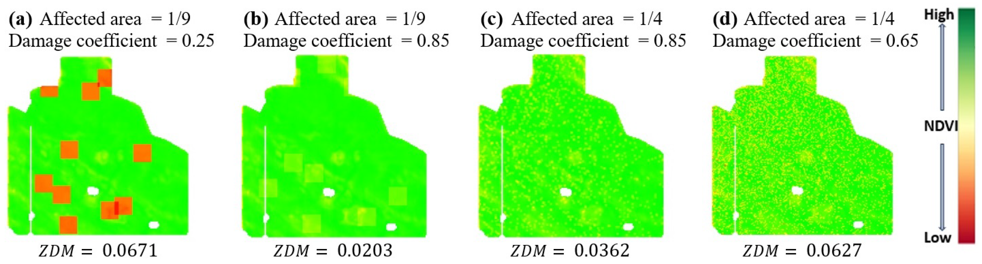
We explored various scenarios using synthetic data, altering the perturbed area and the severity of damage to assess the robustness of our framework. For example, we changed the damaged portion’s location or area within the field. Additionally, we conducted experiments with completely random pixel perturbations. To ensure reliability, we averaged the results of 10 experiments for each random scenario.
Figure 14 shows the results of these experiments, the affected area, and the damage coefficient (the coefficient multiplied by NDVI values). Our framework identified the synthetic year as an abnormal zoning year in (a) and (d). Comparing (a) and (b), only the damage severity was decreased, showing that the decreased accordingly. (c) demonstrates the case when individual pixels are affected, but the severity of the damaged area is not large enough to increase the value significantly. Conversely, in scenario (d), where the severity of damage is higher than that in (c), the value in the synthetic year dramatically increases.
When the synthesized data are the same as the zoning invariant data (), the resulting will be zero. Additionally, if the new data are plus a uniform and global change (e.g., reducing all pixel values by a constant factor), the value will also be zero. Only alternations to that change the relative performance of pixels can potentially change the value.
To illustrate, we synthetically halved the zoning invariant data () for each pixel (see Figure 15a), resulting in a zero value for the synthetic data. Consequently, including these altered data in the zoning process had no impact on the resulting zonemap, as depicted in (b).
6. Conclusions and Future Works
The Zoning Dissimilarity Metric () and the defined framework are potent tools for recognizing abnormal zoning data within historical field records, especially within smaller areas, like fields or subfields. Our various experimental results with real and synthetic data demonstrate the effectiveness of the in detecting changes in field performance in terms of zone changes. Moreover, the is a valuable tool to compare the partial or global relative performance of fields over time.
By harnessing the power of the , we can effectively detect and eliminate anomalous zoning data before identifying management zones. This results in improved accuracy in zone labelling, leading to enhanced precision in resource management across field operations. However, there is room to improve the evaluation of our resulting zonemaps and investigate how the enhanced accuracy in zone labelling and resource management facilitated by the can translate into tangible benefits for farmers.
Furthermore, there is an opportunity to leverage the capability of the to detect the damaged area of the field more accurately in the future. Additionally, future research should explore alternative performance indicators and adaptive thresholding techniques for specific crops or weather conditions, including investigating the adaptability of our framework to cases with more than one growing season. Machine learning techniques can be employed in the `’long term” after collecting data over a longer time frame in this regard.
Author Contributions
Conceptualization, R.H. and F.F.S.; methodology, R.H. and F.F.S.; software, R.H.; validation, R.H. and F.F.S.; writing—review and editing, R.H. and F.F.S.; supervision, F.F.S.; funding acquisition, F.F.S. All authors have read and agreed to the published version of the manuscript.
Funding
MITACS, TELUS Agriculture, Application Ref. IT32167.
Institutional Review Board Statement
Not applicable.
Data Availability Statement
The data used in this study are openly available and were obtained from Sentinel Hub services. The API documentation is available online at: https://docs.sentinel-hub.com/api/latest/data/sentinel-2-l2a/. The shapefiles for the experimental fields are privately owned by the industrial partner.
Acknowledgments
We wish to acknowledge the support of the Mathematics of Information Technology and Complex Systems (MITACS), Decisive Farming (TELUS Agriculture) and the Natural Sciences and Engineering Research Council of Canada (NSERC). We would like to express our sincere thanks to Vincent Yeow Chieh Pang and Garret Duffy for the great discussions and insights during the Mitacs project. Special thanks go out to Christopher Mossman for proofreading the manuscript. We thank all members of the GIV research team at the University of Calgary, specifically Meysam Kazemi, Lakin Wecker, Amirhossein Mirtabatabaeipour, John Hall, and Mohammadreza Osouli, for developing the foundation of the application and all GIV team members for their insights and discussions.
Conflicts of Interest
The authors declare no conflicts of interest.
Abbreviations
The following abbreviations are used in this manuscript:
| AZY | Abnormal Zoning Year |
| BI | Brightness Index |
| CL | Coloration Index |
| CV | coefficient of variation |
| DSA | Data-Driven Soil Assessment |
| GNDVI | Green Normalized Vegetation Index |
| IoT | Internet of Things |
| MLR | Multiple Linear Regression |
| MSI | Moisture Stress Index |
| NDVI | Normalized Difference Vegetation Index |
| NDWI | Normalized Difference Water Index |
| NIR | near-infrared |
| ODI | Optimal Difference Index |
| ONDVI | Optimal Normalized Difference Vegetation Index |
| ORVI | Optimal Ratio Vegetation Index |
| RF | Random Forest |
| SEC | Soil Electrical Conductivity |
| SOC | Soil Organic Carbon |
| SOMC | Soil Organic Matter Content |
| SSCM | Site-Specific Crop Management |
| UAV | Unmanned Aerial Vehicle |
| VRT | variable rate technology |
| ZDM | Zoning Dissimilarity Metric |
Appendix A

Table A1.
measurements and abnormal zoning years.
| ID | 2017 | 2018 | 2019 | 2020 | 2021 | 2022 | AZY | |||
|---|---|---|---|---|---|---|---|---|---|---|
| 1 | 0.0095 | 0.0278 | 0.0115 | 0.0424 | 0.0534 | 0.018 | 0.0271 | 0.0177 | 65.3 | 2020, 2021 |
| 2 | 0.0181 | 0.0294 | 0.0188 | 0.0257 | 0.0503 | 0.0235 | 0.0276 | 0.0119 | 43.1 | 2021 |
| 3 | 0.0218 | 0.0325 | 0.0121 | 0.0142 | 0.0672 | 0.0457 | 0.0322 | 0.0212 | 65.7 | 2021, 2022 |
| 4 | 0.0294 | 0.0500 | 0.0125 | 0.0125 | 0.0297 | 0.0225 | 0.0261 | 0.0140 | 53.5 | 2018 |
| 5 | 0.0294 | 0.0336 | 0.0240 | 0.0108 | 0.0352 | 0.0407 | 0.0290 | 0.0105 | 36.3 | — |
| 6 | 0.0184 | 0.0306 | 0.0170 | 0.0137 | 0.1143 | 0.0152 | 0.0349 | 0.0394 | 112.9 | 2021 |
| 7 | 0.0237 | 0.0430 | 0.0235 | 0.0286 | 0.0272 | 0.0383 | 0.0307 | 0.0081 | 26.2 | — |
| 8 | 0.0244 | 0.0185 | 0.0121 | 0.0146 | 0.0351 | 0.0189 | 0.0206 | 0.0082 | 40.0 | — |
| 9 | 0.0351 | 0.0399 | 0.0140 | 0.0200 | 0.0126 | 0.0550 | 0.0294 | 0.0168 | 57.0 | 2022 |
| 10 | 0.0228 | 0.0323 | 0.0210 | 0.0131 | 0.0297 | 0.0217 | 0.0234 | 0.0068 | 29.2 | — |
| 11 | 0.0215 | 0.0093 | 0.0240 | 0.0477 | 0.0450 | 0.0259 | 0.0289 | 0.0148 | 51.1 | 2020, 2021 |
| 12 | 0.0785 | 0.0314 | 0.1247 | 0.0296 | 0.0245 | 0.0202 | 0.0515 | 0.0417 | 80.9 | 2017, 2019 |
| 13 | 0.0332 | 0.0312 | 0.0236 | 0.0096 | 0.0368 | 0.0268 | 0.0269 | 0.0097 | 36.0 | — |
| 14 | 0.0177 | 0.0270 | 0.0181 | 0.0127 | 0.0599 | 0.0201 | 0.0259 | 0.0173 | 66.7 | 2021 |
| 15 | 0.0213 | 0.0558 | 0.0160 | 0.0238 | 0.0407 | 0.0116 | 0.0282 | 0.0168 | 59.5 | 2018, 2021 |
| 16 | 0.0850 | 0.0199 | 0.0164 | 0.0405 | 0.0500 | 0.0403 | 0.0420 | 0.0248 | 58.9 | 2017, 2021 |
| 17 | 0.0164 | 0.0201 | 0.0189 | 0.0198 | 0.0453 | 0.0147 | 0.0225 | 0.0113 | 50.3 | 2021 |
| 18 | 0.0129 | 0.0197 | 0.0155 | 0.0220 | 0.0294 | 0.0167 | 0.0194 | 0.0059 | 30.3 | — |
| 19 | 0.0084 | 0.0162 | 0.0188 | 0.0190 | 0.0304 | 0.0105 | 0.0172 | 0.0078 | 45.3 | — |
| 20 | 0.0063 | 0.0136 | 0.0159 | 0.0213 | 0.0373 | 0.0107 | 0.0175 | 0.0109 | 62.4 | — |
| 21 | 0.0083 | 0.0227 | 0.0134 | 0.0150 | 0.0200 | 0.0119 | 0.0152 | 0.0053 | 34.9 | — |
| 22 | 0.0060 | 0.0146 | 0.0115 | 0.0120 | 0.0267 | 0.0091 | 0.0133 | 0.0072 | 53.8 | — |
| 23 | 0.0182 | 0.0331 | 0.0136 | 0.0109 | 0.0880 | 0.0264 | 0.0317 | 0.0288 | 90.7 | 2021 |
| 24 | 0.0172 | 0.0300 | 0.0129 | 0.0094 | 0.0510 | 0.0314 | 0.0253 | 0.0154 | 61.0 | 2021 |
| 25 | 0.0209 | 0.0221 | 0.0275 | 0.0075 | 0.0939 | 0.0398 | 0.0353 | 0.0305 | 86.5 | 2021 |
| 26 | 0.0237 | 0.0211 | 0.0203 | 0.0079 | 0.0562 | 0.0309 | 0.0267 | 0.0163 | 61.0 | 2021 |
| 27 | 0.0120 | 0.0358 | 0.0146 | 0.0096 | 0.0907 | 0.0338 | 0.0327 | 0.0305 | 93.4 | 2021 |
| 28 | 0.0186 | 0.0143 | 0.0318 | 0.0195 | 0.0380 | 0.0185 | 0.0235 | 0.0093 | 39.5 | — |
| 29 | 0.0501 | 0.0252 | 0.0198 | 0.0239 | 0.0390 | 0.0091 | 0.0279 | 0.0146 | 52.2 | 2017 |
| 30 | 0.0215 | 0.0148 | 0.0191 | 0.0111 | 0.0502 | 0.0105 | 0.0212 | 0.0148 | 70.0 | 2021 |
| 31 | 0.1000 | 0.0241 | 0.0150 | 0.0132 | 0.0413 | 0.0361 | 0.0383 | 0.0322 | 84.3 | 2017, 2021 |
| 32 | 0.0512 | 0.0160 | 0.0197 | 0.0158 | 0.0576 | 0.0090 | 0.0282 | 0.0207 | 73.2 | 2017, 2021 |
| 33 | 0.0208 | 0.0242 | 0.0209 | 0.0686 | 0.0730 | 0.0300 | 0.0396 | 0.0245 | 61.8 | 2020, 2021 |
| 34 | 0.0576 | 0.0306 | 0.0201 | 0.0139 | 0.0859 | 0.0201 | 0.0380 | 0.0281 | 73.9 | 2017, 2021 |
| 35 | 0.0469 | 0.0221 | 0.0179 | 0.0349 | 0.0445 | 0.0082 | 0.0291 | 0.0155 | 53.3 | 2017, 2021 |
| 36 | 0.0506 | 0.0268 | 0.0128 | 0.0235 | 0.0541 | 0.0154 | 0.0305 | 0.0177 | 58.0 | 2017, 2021 |
| 37 | 0.0157 | 0.0067 | 0.0173 | 0.0955 | 0.0210 | 0.0133 | 0.0283 | 0.0333 | 117.9 | 2020 |
| 38 | 0.0223 | 0.0183 | 0.0183 | 0.0154 | 0.0420 | 0.0340 | 0.0251 | 0.0106 | 42.2 | 2021 |
| 39 | 0.0342 | 0.0158 | 0.0155 | 0.0152 | 0.0345 | 0.0160 | 0.0219 | 0.0097 | 44.3 | — |
References
- Tilman, D.; Balzer, C.; Hill, J.; Befort, B.L. Global food demand and the sustainable intensification of agriculture. Proc. Natl. Acad. Sci. USA 2011, 108, 20260–20264. [Google Scholar] [CrossRef] [PubMed]
- Zhang, N.; Wang, M.; Wang, N. Precision agriculture—A worldwide overview. Comput. Electron. Agric. 2002, 36, 113–132. [Google Scholar] [CrossRef]
- Mulla, D.J. Twenty five years of remote sensing in precision agriculture: Key advances and remaining knowledge gaps. Biosyst. Eng. 2013, 114, 358–371. [Google Scholar] [CrossRef]
- Khosla, R.; Alley, M. Soil-specific nitrogen management on mid-Atlantic coastal plain soils. Better Crops 1999, 83, 6–7. [Google Scholar]
- Koch, B.; Khosla, R.; Frasier, W.; Westfall, D.; Inman, D. Economic Feasibility of Variable-Rate Nitrogen Application Utilizing Site-Specific Management Zones. Agron. J. 2004, 96, 1572–1580. [Google Scholar] [CrossRef]
- Nawar, S.; Corstanje, R.; Halcro, G.; Mulla, D.; Mouazen, A.M. Delineation of Soil Management Zones for Variable-Rate Fertilization: A Review. Adv. Agron. 2017, 143, 175–245. [Google Scholar] [CrossRef]
- Inman, D.; Khosla, R.; Reich, R.; Westfall, D.G. Normalized Difference Vegetation Index and Soil Color-Based Management Zones in Irrigated Maize. Agron. J. 2008, 100, 60–66. [Google Scholar] [CrossRef]
- Vannoppen, A.; Gobin, A. Estimating Yield from NDVI, Weather Data, and Soil Water Depletion for Sugar Beet and Potato in Northern Belgium. Water 2022, 14, 1188. [Google Scholar] [CrossRef]
- Roznik, M.; Boyd, M.; Porth, L. Improving crop yield estimation by applying higher resolution satellite NDVI imagery and high-resolution cropland masks. Remote Sens. Appl. Soc. Environ. 2022, 25, 100693. [Google Scholar] [CrossRef]
- Kazemi, M.; Samavati, F.F. Automatic Soil Sampling Site Selection in Management Zones Using a Multi-Objective Optimization Algorithm. Agriculture 2023, 13, 1993. [Google Scholar] [CrossRef]
- Havlin, J.; Heiniger, R. Soil fertility management for better crop production. Agronomy 2020, 10, 1349. [Google Scholar] [CrossRef]
- Whelan, B. Site-Specific Crop Management. In Pedometrics; Springer International Publishing: Cham, Switzerland, 2018; pp. 597–622. [Google Scholar] [CrossRef]
- Barnes, E.M.; Sudduth, K.A.; Hummel, J.W.; Lesch, S.M.; Corwin, D.L.; Yang, C.; Daughtry, C.S.; Bausch, W.C. Remote-and ground-based sensor techniques to map soil properties. Photogramm. Eng. Remote Sens. 2003, 69, 619–630. [Google Scholar] [CrossRef]
- Li, Y.; Shi, Z.; Li, F.; Li, H.Y. Delineation of site-specific management zones using fuzzy clustering analysis in a coastal saline land. Comput. Electron. Agric. 2007, 56, 174–186. [Google Scholar] [CrossRef]
- Georgi, C.; Spengler, D.; Itzerott, S.; Kleinschmit, B. Automatic delineation algorithm for site-specific management zones based on satellite remote sensing data. Precis. Agric. 2018, 19, 684–707. [Google Scholar] [CrossRef]
- Molin, J.P.; Castro, C.N.d. Establishing management zones using soil electrical conductivity and other soil properties by the fuzzy clustering technique. Sci. Agric. 2008, 65, 567–573. [Google Scholar] [CrossRef]
- Zhang, Q. Precision Agriculture Technology for Crop Farming; Taylor & Francis: Abingdon, UK, 2016. [Google Scholar] [CrossRef]
- Balafoutis, A.T.; Beck, B.; Fountas, S.; Tsiropoulos, Z.; Vangeyte, J.; van der Wal, T.; Soto-Embodas, I.; Gómez-Barbero, M.; Pedersen, S.M. Smart farming technologies–description, taxonomy and economic impact. In Precision Agriculture: Technology and Economic Perspectives; Springer: Cham, Switzerland, 2017; pp. 21–77. [Google Scholar] [CrossRef]
- Cammarano, D.; Zha, H.; Wilson, L.; Li, Y.; Batchelor, W.D.; Miao, Y. A remote sensing-based approach to management zone delineation in small scale farming systems. Agronomy 2020, 10, 1767. [Google Scholar] [CrossRef]
- Wadoux, A.M.C.; Molnar, C. Beyond prediction: Methods for interpreting complex models of soil variation. Geoderma 2022, 422, 115953. [Google Scholar] [CrossRef]
- Xue, J.; Su, B. Significant remote sensing vegetation indices: A review of developments and applications. J. Sensors 2017, 2017, 1353691. [Google Scholar] [CrossRef]
- Jin, X.; Du, J.; Liu, H.; Wang, Z.; Song, K. Remote estimation of soil organic matter content in the Sanjiang Plain, Northest China: The optimal band algorithm versus the GRA-ANN model. Agric. For. Meteorol. 2016, 218–219, 250–260. [Google Scholar] [CrossRef]
- Srisomkiew, S.; Kawahigashi, M.; Limtong, P.; Yuttum, O. Digital soil assessment of soil fertility for Thai jasmine rice in the Thung Kula Ronghai region, Thailand. Geoderma 2022, 409, 115597. [Google Scholar] [CrossRef]
- Rembold, F.; Atzberger, C.; Savin, I.; Rojas, O. Using low resolution satellite imagery for yield prediction and yield anomaly detection. Remote Sens. 2013, 5, 1704–1733. [Google Scholar] [CrossRef]
- Layton, J.C.; Wecker, L.; Runions, A.; Samavati, F.F. Cloud Shadow Detection via Ray Casting with Probability Analysis Refinement Using Sentinel-2 Satellite Data. Remote Sens. 2023, 15, 3955. [Google Scholar] [CrossRef]
- Wecker, L.; Samavati, F.; Gavrilova, M. Contextual void patching for digital elevation models. Vis. Comput. 2007, 23, 881–890. [Google Scholar] [CrossRef]
- Vilenski, E.; Bak, P.; Rosenblatt, J.D. Multivariate anomaly detection for ensuring data quality of dendrometer sensor networks. Comput. Electron. Agric. 2019, 162, 412–421. [Google Scholar] [CrossRef]
- Moso, J.C.; Cormier, S.; de Runz, C.; Fouchal, H.; Wandeto, J.M. Anomaly Detection on Data Streams for Smart Agriculture. Agriculture 2021, 11, 1083. [Google Scholar] [CrossRef]
- Catalano, C.; Paiano, L.; Calabrese, F.; Cataldo, M.; Mancarella, L.; Tommasi, F. Anomaly detection in smart agriculture systems. Comput. Ind. 2022, 143, 103750. [Google Scholar] [CrossRef]
- Schroth, C.; Kelbert, P.; Vollmer, A.M. A data quality assessment tool for agricultural structured data as support for smart farming. In Resiliente Agri-Food-Systeme, Lecture Notes in Informatics (LNI); Gesellschaft für Informatik e.V.: Bonn, Germany, 2023. [Google Scholar]
- Peters, A.J.; Walter-Shea, E.A.; Ji, L.; Vina, A.; Hayes, M.; Svoboda, M.D. Drought monitoring with NDVI-based standardized vegetation index. Photogramm. Eng. Remote Sens. 2002, 68, 71–75. [Google Scholar]
- Shrestha, R.; Di, L.; Yu, G.; Shao, Y.; Kang, L.; Zhang, B. Detection of flood and its impact on crops using NDVI-Corn case. In Proceedings of the 2013 Second International Conference on Agro-Geoinformatics (Agro-Geoinformatics), Fairfax, VA, USA, 12–16 August 2013; pp. 200–204. [Google Scholar] [CrossRef]
- Buresh, R.J.; Sánchez, P.A.; Calhoun, F. Replenishing Soil Fertility in Africa; Citeseer: Princeton, NJ, USA, 1997; Volume 51, pp. 12–17. Available online: https://citeseerx.ist.psu.edu/document?repid=rep1&type=pdf&doi=39d64a6784ecc0c0bb82aaa05eb0575439bc46cf (accessed on 23 April 2024).
- Pedersen, S.M.; Lind, K.M. Precision Agriculture: Technology and Economic Perspectives; chapter Sustainable Intensification in Crop Farming; Springer: Cham, Switzerland, 2017; pp. 597–608. [Google Scholar] [CrossRef]
- Hird, J.; Mcdermid, G. Noise reduction of NDVI time series: An empirical comparison of selected techniques. Remote Sens. Environ. 2009, 113, 248–258. [Google Scholar] [CrossRef]
- Ryu, J.H.; Jeong, H.; Cho, J. Performances of vegetation indices on paddy rice at elevated air temperature, heat stress, and herbicide damage. Remote Sens. 2020, 12, 2654. [Google Scholar] [CrossRef]
- Schmaltz, T.; Melnitchouk, A. Variable Zone Crop-Specific Inputs Prescription Method and Systems Therefor. CA Patent 2663917, 30 December 2014. [Google Scholar]
- Gatti, A.; Bertolini, A. Sentinel-2 Products Specification Document. 2013. Available online: https://sentinel.esa.int/documents/247904/349490/S2_MSI_Product_Specification.pdf (accessed on 23 December 2023).
- Fridgen, J.J.; Kitchen, N.R.; Sudduth, K.A.; Drummond, S.T.; Wiebold, W.J.; Fraisse, C.W. Management zone analyst (MZA) software for subfield management zone delineation. Agron. J. 2004, 96, 100–108. [Google Scholar] [CrossRef]
- Spearman, C. The proof and measurement of association between two things. Am. J. Psychol. 1904, 15, 72–101. [Google Scholar] [CrossRef]
- Spearman, C. “General Intelligence” Objectively Determined and Measured. Am. J. Psychol. 1961, 15, 59–73. [Google Scholar] [CrossRef]
- Guo, Y.; Li, Z. A lognormal model for evaluating maximum residue levels of pesticides in crops. Environ. Pollut. 2021, 278, 116832. [Google Scholar] [CrossRef] [PubMed]
- Jalilibal, Z.; Amiri, A.; Castagliola, P.; Khoo, M.B. Monitoring the coefficient of variation: A literature review. Comput. Ind. Eng. 2021, 161, 107600. [Google Scholar] [CrossRef]
- Aureli, R.; Brandizzi, N.; De Magistris, G.; Brociek, R. A customized approach to anomalies detection by using autoencoders. In Proceedings of the CEUR Workshop Proceedings, CEUR-WS, Catania, Italy, 27–29 July 2021; Volume 3092, pp. 53–59. [Google Scholar]
- Mishra, P.; Homa, F. Essentials of Statistics in Agriculture Sciences, 1st ed.; Apple Academic Press: Cambridge, MA, USA, 2019; pp. 11, 18, 26. [Google Scholar] [CrossRef]
- Government, C. Canadian Drought Monitor. Available online: https://agriculture.canada.ca/en/agricultural-production/weather/canadian-drought-monitor/drought-analysis (accessed on 25 July 2023).
- Solh, M.; Ginkel, M.V. Drought preparedness and drought mitigation in the developing world’s drylands. Weather. Clim. Extrem. 2014, 3, 62–66. [Google Scholar] [CrossRef]
- Ha, T.; Shen, Y.; Duddu, H.; Johnson, E.; Shirtliffe, S.J. Quantifying Hail Damage in Crops Using Sentinel-2 Imagery. Remote Sens. 2022, 14, 951. [Google Scholar] [CrossRef]
Figure 1.
A sample zonemap after zoning. This field is classified by six labels from zone 1 to 6.

Figure 2.
Abnormal zoning year(s) detection framework.

Figure 3.
Results of zoning with different zone numbers. (a) Zonemap for . (b) Zonemap for .

Figure 4.
Altering input images changes the zonemap.

Figure 5.
A field’s boundary: The area denoted by D shows the field. The square around the shape of the field is the bounding box. Point p is a pixel in the field’s boundary, and is a pixel out of the boundary. All out-of-boundary pixels are excluded in the calculations, i.e., Equation (4).
Figure 5.
A field’s boundary: The area denoted by D shows the field. The square around the shape of the field is the bounding box. Point p is a pixel in the field’s boundary, and is a pixel out of the boundary. All out-of-boundary pixels are excluded in the calculations, i.e., Equation (4).

Figure 6.
The distribution of values. (a) The histogram of raw values shows a log-normal distribution shape. (b) The histogram plot of transformed values using a natural logarithm. The plot shows that the transformed data are normally distributed.
Figure 6.
The distribution of values. (a) The histogram of raw values shows a log-normal distribution shape. (b) The histogram plot of transformed values using a natural logarithm. The plot shows that the transformed data are normally distributed.

Figure 7.
Abnormality conditions based on the measured values. A list named is the output of the algorithm.
Figure 7.
Abnormality conditions based on the measured values. A list named is the output of the algorithm.

Figure 8.
Studied fields: Each flagged point shows one field. Some fields are overlapped. Map data: ©2024 Google.
Figure 8.
Studied fields: Each flagged point shows one field. Some fields are overlapped. Map data: ©2024 Google.

Figure 9.
Canada Drought Monitoring [46]. (a) Drought conditions in July 2021, which was a drought year. (b) Drought conditions in July 2020, which was a normal year.
Figure 9.
Canada Drought Monitoring [46]. (a) Drought conditions in July 2021, which was a drought year. (b) Drought conditions in July 2020, which was a normal year.

Figure 10.
values for the experimental fields over two years. The X-axis has each field’s ID. The orange line is the mean of the values for all years. (Left) values for the drought year. (Right) values for a normal year.
Figure 10.
values for the experimental fields over two years. The X-axis has each field’s ID. The orange line is the mean of the values for all years. (Left) values for the drought year. (Right) values for a normal year.

Figure 11.
Three different performance function visualizations for each year in one field. values are calculated for each case.
Figure 11.
Three different performance function visualizations for each year in one field. values are calculated for each case.

Figure 12.
Peak green for all years from 2017 to 2022 plus synthetic year. values for each data are calculated.
Figure 12.
Peak green for all years from 2017 to 2022 plus synthetic year. values for each data are calculated.

Figure 13.
The effect of data from synthetic years on the zoning. (a) The synthetic data. (b) The zonemap without including the synthetic data. (c) The zonemap after including the synthetic data. (d) The difference between zonemaps.
Figure 13.
The effect of data from synthetic years on the zoning. (a) The synthetic data. (b) The zonemap without including the synthetic data. (c) The zonemap after including the synthetic data. (d) The difference between zonemaps.

Figure 14.
Various scenarios of synthetic data. (a–d) The affected area and damage coefficient are indicated, and values for each scenario are calculated.
Figure 14.
Various scenarios of synthetic data. (a–d) The affected area and damage coefficient are indicated, and values for each scenario are calculated.

Figure 15.
(a) A uniform change in the performance data is created synthetically. The of the synthetic data is zero. (b) The zonemap before and after including the synthetic data in the zoning.
Figure 15.
(a) A uniform change in the performance data is created synthetically. The of the synthetic data is zero. (b) The zonemap before and after including the synthetic data in the zoning.

Table 1.
Zonemap changes. () Zonemap after altering the input dataset. () The baseline zonemap. (c) Zone change extent. (d) Change intensity. The green pixels signify an increase in the zone label (e.g., from zone 4 to 5), while reddish pixels indicate a decrease in the zone label (e.g., from zone 5 to 4 or, in darker orange pixels, to 3). Yellow pixels denote unchanged labels.
| I | c | d | ||
|---|---|---|---|---|
 |  |  |  | |
 |  |  |  |
Table 2.
Six of our study fields’ locations (sampled from thirty-nine total fields).
| Field | Shape | BBox | BBox | Province | Area |
|---|---|---|---|---|---|
| ID | Bottom Left | Top Right | (Acres) | ||
| 1 |  | (−113.497, 51.343) | (−113.474, 51.357) | Alberta | 491 |
| 2 |  | (−105.921, 52.710) | (−105.909, 52.718) | Saskatchewan | 155 |
| 3 |  | (−107.905, 51.685) | (−107.894, 51.692) | Saskatchewan | 159 |
| 4 |  | (−111.949, 50.096) | (−111.934, 50.106) | Alberta | 216 |
| 5 |  | (−109.037, 52.318) | (−109.025, 52.325) | Saskatchewan | 166 |
| 6 |  | (−108.859, 52.143) | (−108.847, 52.150) | Saskatchewan | 156 |
Table 3.
measurements and abnormal zoning years.
| ID | 2017 | 2018 | 2019 | 2020 | 2021 | 2022 | AZY | |||
|---|---|---|---|---|---|---|---|---|---|---|
| 1 | 0.0095 | 0.0278 | 0.0115 | 0.0424 | 0.0534 | 0.018 | 0.0271 | 0.0177 | 65.3 | 2020, 2021 |
| 2 | 0.0181 | 0.0294 | 0.0188 | 0.0257 | 0.0503 | 0.0235 | 0.0276 | 0.0119 | 43.1 | 2021 |
| 3 | 0.0218 | 0.0325 | 0.0121 | 0.0142 | 0.0672 | 0.0457 | 0.0322 | 0.0212 | 65.7 | 2021, 2022 |
| 4 | 0.0294 | 0.0500 | 0.0125 | 0.0125 | 0.0297 | 0.0225 | 0.0261 | 0.0140 | 53.5 | 2018 |
| 5 | 0.0294 | 0.0336 | 0.0240 | 0.0108 | 0.0352 | 0.0407 | 0.0290 | 0.0105 | 36.3 | — |
| 6 | 0.0184 | 0.0306 | 0.0170 | 0.0137 | 0.1143 | 0.0152 | 0.0349 | 0.0394 | 112.9 | 2021 |
Disclaimer/Publisher’s Note: The statements, opinions and data contained in all publications are solely those of the individual author(s) and contributor(s) and not of MDPI and/or the editor(s). MDPI and/or the editor(s) disclaim responsibility for any injury to people or property resulting from any ideas, methods, instructions or products referred to in the content. |
© 2024 by the authors. Licensee MDPI, Basel, Switzerland. This article is an open access article distributed under the terms and conditions of the Creative Commons Attribution (CC BY) license (https://creativecommons.org/licenses/by/4.0/).
Share and Cite
MDPI and ACS Style
Heidari, R.; Samavati, F.F. A New Dissimilarity Metric for Anomaly Detection in Management Zones Delineation Constructed from Time-Varying Satellite Images. Agriculture 2024, 14, 688. https://doi.org/10.3390/agriculture14050688
AMA Style
Heidari R, Samavati FF. A New Dissimilarity Metric for Anomaly Detection in Management Zones Delineation Constructed from Time-Varying Satellite Images. Agriculture. 2024; 14(5):688. https://doi.org/10.3390/agriculture14050688
Chicago/Turabian StyleHeidari, Roghayeh, and Faramarz F. Samavati. 2024. "A New Dissimilarity Metric for Anomaly Detection in Management Zones Delineation Constructed from Time-Varying Satellite Images" Agriculture 14, no. 5: 688. https://doi.org/10.3390/agriculture14050688
Note that from the first issue of 2016, this journal uses article numbers instead of page numbers. See further details here.