
Solar Filament Detection Based on an Improved Deep Learning Model

1
Faculty of Information Engineering and Automation, Kunming University of Science and Technology, Kunming 650500, China
2
Yunnan Key Laboratory of Artificial Intelligence, Kunming University of Science and Technology, Kunming 650500, China
*
Author to whom correspondence should be addressed.
Appl. Sci. 2024, 14(9), 3745; https://doi.org/10.3390/app14093745
Submission received: 5 April 2024
/
Revised: 24 April 2024
/
Accepted: 25 April 2024
/
Published: 27 April 2024
Abstract
:Solar filaments are good tracers of space weather and magnetic flux ropes in the corona. Identifying and detecting filaments helps to forecast space weather and explore the solar magnetic field. Many automatic detection methods have been proposed to process the large number of observed images. Current methods face issues of unreliable dataset annotations and poor anti-interference capability. First, to address the issue of unreliable dataset annotations, we built a solar filament dataset using a manual annotation method. Second, we introduced Transformer into Convolutional Neural Networks. Transformer, with the ability to extract more global features, can help counter interference. In addition, there is large disparity in the size of solar filaments. Therefore, a multi-scale residual block is designed to extract features across various scales. Deformable large kernel attention and a res path are used to better integrate encoder and decoder information. Results show that this method outperforms the existing solar filament detection methods (improved U-Net and improved V-Net), achieving an F1 score of 91.19%. In particular, our results show lower interference by sunspots and background noise than existing methods. The ability to counter interference is improved.
1. Introduction
Solar filaments are composed of low-temperature, high-density plasma [1,2]. They are closely related to space weather. Eruptions of solar filaments are extremely spectacular solar events that cause plasma ejection. The plasma ejected during eruptions can reach Earth within a few days, thus influencing Earth’s magnetosphere. In severe cases, this can lead to disasters such as communication disruptions and navigation failures [3,4,5,6]. In addition, solar filaments serve as carriers of magnetic free energy that is accumulated and stored within the corona, and they are one of the best tracers of magnetic flux ropes in the corona [7,8,9,10]. Detection of solar filaments helps forecasters forecast space weather and explore the solar magnetic field. As solar observing equipment advances and the number of observed images grows, automatic detection of solar filaments becomes more important. Many methods have been proposed to process the large number of observed images automatically.
Due to the dark color of solar filaments observed through the Hα (6563 Å) spectral line, most existing methods use full-disk Hα images as input to detect solar filaments. The specific methods can be divided into three categories:
- Threshold-based segmentation methods. Researchers use threshold-based methods such as global thresholding, local thresholding, and adaptive thresholding to detect solar filaments [11,12,13,14,15]. Some methods also combine techniques such as mathematical morphology, region growing, and edge detection [16]. However, these methods are prone to misidentifying noise in the images as filaments, resulting in poor detection results. There are quite significant differences between the detection results and the actual results, which can easily mislead astronomers;
- Machine learning-based methods. For instance, artificial neural networks are used to detect filaments [17,18]. Such methods can efficiently extract features using appropriate feature extractors designed with prior knowledge. They also have fast model training speeds. However, feature extractors should be designed with rich prior knowledge during usage. Additionally, they have poor model generalization, and their detection results are susceptible to interference when facing more complex characteristics. The methods are not conducive to large-scale application, and the detection results still need to be improved;
- Deep learning-based methods. Deep learning methods can better extract image characteristics and have achieved great success in image processing, attracting widespread attention from scholars [19,20,21]. Researchers have employed Convolutional Neural Networks (CNN) to investigate solar filament detection methods. Many methods have been proposed based on CNN models, such as Mask R-CNN [22], U-Net [23], V-Net [24], CondInst [25], and so on. Researchers have also used methods based on unsupervised and semi-unsupervised learning, but found the results were not as good as those based on CNN [26]. In contrast to machine learning methods, deep learning methods have higher generalization and robustness. They also have better detection results. However, these methods rely on accurate dataset annotations. Current methods suffer from the unreliability of annotations in existing datasets. Moreover, they have poor anti-interference capability. This often leads to issues such as incorrect detection of sunspots as solar filaments, loss of small filaments, and incorrect detection of background noise as solar filaments.
Overall, among the existing solar filament detection methods, those based on deep learning exhibit the best detection performance and have become the most popular in the last three years. Therefore, this study uses a deep learning-based method to detect solar filaments. The goal of this method is to address the following two issues faced by existing methods: unreliable dataset annotations and interference from sunspots and background noise.
We built a new solar filament dataset and proposes a Hybrid CNN-Transformer model for filament detection. The model introduces Transformer, designs a multi-scale residual block, and introduces deformable large kernel attention along with the res path. All of the structures are specifically designed for the characteristics of solar filaments.
Experiments were conducted on full-disk Hα images observed by the Big Bear Solar Observatory (BBSO) from 2012 to 2014. Our method achieved accurate detection of solar filaments, especially in the presence of sunspot interference and background noise, with detection performance superior to the existing methods Improved U-Net and Improved V-Net. In practical applications, it can detect filaments from observed images by BBSO automatically and accurately.
The structure of this study is as follows: Section 2 shows the problems of existing datasets, as well as the process of building a new dataset. Section 3 introduces the Hybrid CNN-Transformer Model and explains why it works well for the task of filament detection. Section 4 delves into the method and introduces the structure of the model. In Section 5, discussions and explanations are provided regarding the detection results. Finally, the conclusion is presented in Section 6.
2. Dataset
2.1. Problems with Existing Solar Filament Datasets
Deep learning-based methods rely on dataset annotations to extract the features of filaments. Unreliable annotations can lead to errors in the detection results.
Currently, there are two publicly available solar filament datasets. One is the dataset maintained by the Huairou Solar Observing Station (hereinafter referred to as Dataset 1) [23]. The other is the dataset published in reference [24] (hereinafter referred to as Dataset 2). Dataset 1 uses a threshold segmentation method for annotation. There are numerous errors in the annotations. Dataset 2 uses a manual annotation method, but a considerable number of filaments are missed. Figure 1 shows randomly selected images from the aforementioned two solar filament datasets. In Figure 1, the yellow rectangles represent incorrect annotations where non-filamentary parts are falsely annotated as filaments. The white rectangles indicate erroneous annotations where sunspots are mistakenly annotated as filaments, and the red rectangles indicate missed annotations for solar filaments.
These incorrect annotations in the dataset can easily affect the accuracy of solar filament detection results. Therefore, we felt it necessary to build a new dataset.
2.2. Dataset Building
To avoid the impact of unreliable dataset annotations, we built a new solar filament dataset. It includes 150 pairs of full-disk Hα images and their annotations, observed by BBSO from 2012 to 2014. BBSO provides two types of full-disk Hα images, as shown in Figure 2. One is the raw, unprocessed images, as depicted in Figure 2a. The other is the preprocessed images, with limb darkening and brightness inhomogeneity removed, as shown in Figure 2b. It can be observed that the preprocessed images exhibit clearer filament structures. Therefore, we adopted the preprocessed full-disk Hα images.
Solar observations can be affected by various factors, including the rotation and revolution of the Earth, atmospheric conditions, and lighting environments. Consequently, position of the solar disk may vary in different images. Therefore, we performed preprocessing on the full-disk Hα images. First, the solar disk is shifted to the center of the image. Both the Hough circle detection method and the least squares fitting method are used to get the position of solar disk. Then the solar disk will be moved to the center of the image. If the fitting results obtained by the two methods differ by more than five pixels, a manual adjustment is performed. Images where the solar disk position exceeds the image edge are discarded. Next, pixels outside the solar disk are set to gray to avoid interference from prominences. Finally, the ROF denoise is applied. The images before and after preprocessing are shown in Figure 3. It can be observed from Figure 3 that the preprocessed images are more conducive to the detection of solar filaments.
We manually annotated filaments using the LabelMe tool. Repeated manual inspections of the annotation results were conducted to prevent the omission of filaments during the annotation process. Figure 4 presents an example of a full-disk Hα image along with its corresponding filament annotation.
The dataset includes 150 sets of Hα images and their corresponding manual annotation images, all 512 × 512 in size and in PNG format. The Hα images were observed between 2012 and 2014. The annotation images are binary images, representing two classes: The white pixels represent filament annotations, while the black pixels represent non-filament areas. The dataset differs from those used in other semantic segmentation applications. In the annotations, filament annotations only account for an average of 8% of total images, and they are small in size. Therefore, it is necessary to specifically design methods tailored for filament detection. More features related to filaments will be introduced in Section 3.
3. Hybrid CNN-Transformer Model
3.1. CNN
Existing deep learning-based solar filament detection methods are based on CNN. CNN uses convolution operations to extract features.
Convolutional operations can be seen as linear functions parameterized by the convolution kernel W. There are also structures such as pooling layers and activation functions that add nonlinearity to the model. By stacking these layers, CNN models can be regarded as nonlinear mappings with a large number of parameters. They map the input image to the result image. The values of parameters are determined through gradient descent progress while training. After training, by inputting images into this model, we can obtain the output result images.
Due to the limitations of convolution operations, CNN tends to focus more on local details such as textures and edges. It is unable to effectively utilize global information like overall structure.
3.2. Transformer
In recent years, Transformer [27], which uses Transformer layers instead of convolutional operations, has become a popular deep learning model. The structure of the Transformer layer is illustrated in the Figure 5. It requires vectors as input, and focuses more on the relationships among the input vectors through Multi-Head Self-Attention (MSA), Multi-Layer Perceptron (MLP), and Layer Normalization (LN).
Transformer is capable of capturing dependencies between various positions in the input sequence, thereby establishing a global receptive field and exhibiting strong global information extraction capabilities. Vision Transformer [28] applied the Transformer to the field of computer vision. It achieved promising results, inspiring a large number of computer vision models based on the Transformer. However, when processing images, the Transformer only captures features with relatively large grain size. This results in the loss of much local detail information.
3.3. Hybrid CNN-Transformer Model
Figure 6 shows a full-disk Hα image observed on 21 October 2013 at 19:50:25 UT. The filaments in the four red boxes were selected for analysis: a broken, long filament in box 1, a large flaky filament in rectangle 2, a broken circular filament in rectangle 3, and a small filament in rectangle 4. The structures within rectangles 5 and 6 are sunspots. They are similar to filaments. When manually detecting these filaments, it is necessary to use detailed features such as the brightness and edges of the filaments. It is also important to consider global features such as shapes and overall structure.
Existing methods are less capable of utilizing global features. They are prone to be overly sensitive to local features, resulting in misdetections of background noise and sunspots such as the structures in rectangles 5 and 6. Therefore, fully utilizing global features will improve the method’s resistance to interference.
To effectively combine local detail information with global information, researchers have experimented with introducing Transformer into CNN, leading to the development of various Hybrid CNN-Transformer models. Among these, SETR [29] and TransUnet [30] are notable examples. SETR employs Transformer for feature encoding and employs CNN to decode the global information obtained from Transformer. TransUnet inserts Transformer between the encoder and decoder of U-Net, leveraging the local detail information extracted by the U-Net encoder as the input features for Transformer.
Introducing Transformer into CNN can enable the network to combine global information with local detail information. We applied this method to the field of solar filament detection. It can better deal with features of the textures, edges, locations, and structures of solar filaments, thus achieving better solar filament detection performance.
4. Method
Based on the characteristics of solar filaments and the issues surrounding their detection, we designed a Hybrid CNN-Transformer detection model. The structure of the detection model proposed in this article is shown in Figure 7.
As shown in Figure 7, the detection model proposed in this article can be divided into four parts: CNN Encoder, Transformer Encoder, CNN Decoder, and Res Path.
The CNN Encoder uses three sets of Multi-scale Residual Blocks (MRB) to extract features from the input image. It down-samples the input feature map from its original size of (3, W, H) to (64, W/2, H/2), (256, W/4, H/4), and (512, W/8, H/8), obtaining feature maps that contain local detail information about solar filaments as extracted by CNN. Subsequently, by connecting the CNN Encoder and Transformer Encoder in series, the model leverages the powerful global receptive field of the Transformer to capture the global information of solar filaments. In the CNN Decoder, the Decoder Block is used to up-sample the image feature maps and restore their feature sizes, gradually increasing the image size from (512, W/8, H/8) to its original size. The res path implements skip connections, also mitigating the semantic gap between the feature maps obtained from the encoder and those from the decoder. Detailed introductions to each part of the network are provided below.
4.1. CNN Encoder
The CNN Encoder is responsible for extracting local detail information from the input full-disk Hα image and reducing its size while preserving the feature maps for skip connections.
Solar filaments exhibit various sizes in full-disk Hα images, making it challenging to select an appropriate convolution kernel size. Large-sized solar filaments have their information distributed over a larger area, making larger convolution kernels suitable for feature extraction. Smaller-sized solar filaments have their information concentrated in a smaller area, necessitating the use of smaller convolution kernels for feature extraction. It is necessary to enhance the multi-scale feature extraction capability of the CNN Encoder. Therefore, this article proposes using a multi-scale residual block (MRB). The MRB utilizes parallel convolution and pooling kernels of different sizes to extract the features of solar filaments. Its structure is illustrated in Figure 8.
In the MRB, the input image is first processed through three different paths, involving 3 × 3 convolution, 3 × 3 pooling, and 5 × 5 convolution, respectively. The use of different kernel sizes allows for the extraction of solar filament features at various scales. 1 × 1 convolutions after these convolution and pooling layers adjust the output depth, which helps reduce the overall number of network parameters and improves computational efficiency. The solar filament features processed through each of the three paths are then concatenated, forming a multi-scale feature map. Using a 1 × 1 convolution after feature concatenation enables the fusion of solar filament features across different scales, assisting the network in better understanding the global patterns and structures of solar filaments. The addition of a residual path addresses the issues of gradient vanishing and gradient explosion in deep network training, overcoming the problem of overfitting caused by a limited number of data samples.
The detailed structure of the CNN Encoder is presented in Table 1. It employs three sets of MRBs for feature extraction, gradually increasing the number of feature channels.
4.2. Transformer Encoder
The Transformer Encoder is responsible for extracting global features from the solar filament features obtained by the CNN Encoder. Since the Transformer layer requires vectors as input, the filament features need to be serialized before being fed into the Transformer layers. First, the input filament features are sliced into N feature blocks based on a preset slicing size parameter p, where , and each feature block has a dimension of . Here, (C, W, H) represents the shape of the input solar filament features. Subsequently, a trainable linear projection is applied to each feature block to linearly map the feature into a series of feature sequences. Additionally, since the self-attention mechanism does not capture spatial positional relationships, the positional information of each feature block needs to be encoded and embedded into the corresponding position. This process can be represented by the Formula (1).
Here, represents the output sequence, represents the Nth slice, is the trainable linear projection, and is the embedded positional encoding. For each slice, it is transformed into a vector form through a trainable matrix . is used to record the original position of the slices.
12 stacked Transformer layers are used in this part. The outputs are then reshaped for the CNN Decoder.
4.3. CNN Decoder
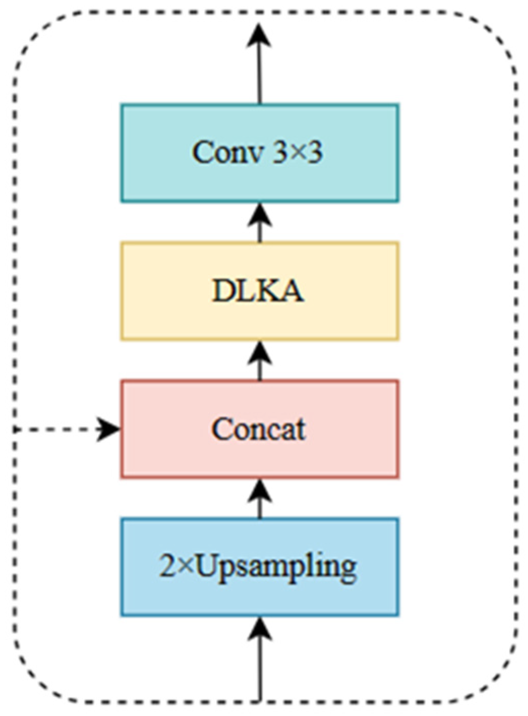
The CNN Decoder uses Decoder Blocks to restore the size of the image while integrating the information provided by the skip connections. The structure of the Decoder Block is shown in Figure 9.
In the Decoder Block, the feature is first enlarged using a 2 × 2 linear interpolation. Subsequently, feature concatenation is performed with the skip connection. Additionally, a Deformable Large Kernel Attention (DLKA) [31] is employed to better integrate the feature with the information from the skip connection. Finally, a 3 × 3 convolution is used to extract features and adjust the number of feature channels.
During training of the model, continuous convolving can easily lead to the loss of filament edges and detailed information. However, information in different spatial locations in the filament feature map is of varying degrees of importance and should therefore be assigned different weights. The integration of an attention mechanism into the network can adjust the weights of different locations in the filament feature map, focusing on key feature areas with high weights and ignoring irrelevant information with low weights. By incorporating DLKA into the Decoder Block, the network can pay attention to the key features of filaments while better integrating local detail information preserved by the CNN Encoder with high-level global features in the CNN Decoder.
During solar filament feature extraction, the larger the convolution kernel size, the more comprehensive the information that the model can access. However, using large-size convolution kernels may introduce too many model parameters and reduce training efficiency. To avoid this issue, large kernel convolution can be decomposed into depthwise convolutions [32], depthwise dilated convolutions, and 1 × 1 convolutions. This decomposition method can effectively reduce the number of parameters while achieving equivalent convolutional effects to large-size convolution kernels [33]. Figure 10 demonstrates the process of decomposing a 7 × 7 large kernel convolution into a 3 × 3 depthwise convolution, a 3 × 3 depthwise dilated convolution, and a 1 × 1 convolution.
While decomposing a large kernel convolution, DLKA introduces deformable convolutions into the depth convolution [34]. The structure of DLKA is shown in Figure 11, which is composed of a deformable depth convolution (Deform-DW Conv), a deformable depth dilation convolution (Deform-DW-D Conv), and a 1 × 1 convolution.
The structure of the deformable depthwise convolution (Deform-DW Conv) is shown within the dashed box in Figure 11. It adds offsets to the depthwise convolution kernel, allowing adaptive adjustment of the kernel shape, thus accommodating the variable shapes of the solar filaments. The deformable depthwise dilated convolution (Deform-DW-D Conv) is similar to the deformable depthwise convolution, except that it uses a depthwise convolution kernel with a dilation rate. Subsequently, an attention map is obtained through a 1 × 1 convolution. Finally, the obtained attention map is multiplied with the input solar filament features to adjust the weights of different locations in the feature map.
DLKA uses deformable convolutions to adapt to different shapes of solar filaments and can adjust the attention weights channel by channel. The method described in this article uses DLKA in CNN Decoder to help the model pay more attention to solar filament features while suppressing unnecessary information and fully integrating encoder and decoder information.
4.4. Res Path
The res path was first proposed by N. Ibtehaz and M.S. Rahman in MultiResUNet [35]. The authors pointed out that in the encoder-decoder architecture, the encoder captures lower-level semantic features while the decoder captures higher-level semantic features. There exists a semantic gap between the two. It is not suitable to combine the encoder features with the decoder features in a straightforward manner. To address this issue, the authors suggested adding a few convolutional layers to the skip connections, leveraging these layers to adjust the features in the skip connections. Using a res path can reduce the semantic differences between the encoder and decoder on feature integration.
The method proposed in this article also has an encoder-decoder architecture. Moreover, it integrates the distinct characteristics of CNN and Transformer, which can further enlarge the semantic gap between the encoder and decoder. Therefore, we employ the res path to establish skip connections between the encoder and decoder. The structure of the res path is illustrated in Figure 12. By utilizing 1 × 1 and 3 × 3 convolutions, it assists the network in processing skip connection information from different scales.
The intensity of the semantic gap between the encoder and decoder feature maps is likely to decrease as moving toward the deeper layers. Therefore, the number of convolutional blocks used along the res paths will gradually reduce. In particular, the method proposed in this article uses 3, 2, and 1 convolutional blocks, respectively, along the three res paths.
5. Results and Discussion
The method described in this article first trains the model, then evaluates the model’s performance based on the testing results.
5.1. Data
Using the solar filament dataset built as described earlier in this article for training, we divided the 150 images into training, validation, and testing sets in the ratio of 6:2:2, resulting in 90, 30, and 30 images in each set, respectively. However, due to the challenging nature of annotating solar filaments and the high cost of manual labeling, the number of images in the dataset was limited. Therefore, data augmentation techniques were employed to expand the training set.
Before training, various augmentation methods were applied, including rotation, vertical flipping, brightness adjustment, and contrast adjustment. These operations effectively increased the diversity of the training data, generating a total of 2700 training samples from the original 90 training images. Rotation and vertical flipping enabled the network to capture image features from various angles and directions, while brightness and contrast adjustments simulated diverse lighting and exposure conditions.
Using these data augmentation techniques, we not only enriched the diversity of the training data but also significantly improved the generalization and robustness of the model.
5.2. Training
The training process was conducted within the PyTorch deep learning framework. The experimental setup employed a Linux-based system with the following hardware specifications: an Intel(R) Xeon(R) CPU running at 2.00 GHz, a Tesla P100 graphics card, and 16 GB of RAM.
For the network’s preset parameters, a batch size of 4 was used for training, and the training process was iterated 150 times. The initial learning rate was set to 0.001. The input image size was set to 512 × 512, and in the Transformer, the patch embedding block size (p) was set to 16. The number of Transformer layers (n) was set to 12, and the dropout rate was set to 0.1.
5.3. Evaluation Metrics
After training, the model can be used for practical applications. It can map the input full-disk Hα images to result images. We evaluated the model’s performance using the detection results of the test set. Evaluation metrics were used to calculate the deviation between the result images and the annotations.
Three performance evaluation metrics—precision, recall, and F1 score—are introduced to objectively and quantitatively assess the detection results of the proposed method. Precision represents the ratio of correctly predicted solar filament pixels to all pixels predicted as solar filaments. A higher precision indicates a more accurate detection of solar filament pixels by the method. Recall measures the proportion of correctly predicted solar filament pixels to the actual number of solar filament pixels. A higher recall indicates fewer omissions in the detection of solar filament pixels. The F1 score, which is calculated based on precision and recall, is used to evaluate the similarity between the detection results and the true labels, providing a comprehensive assessment of the detection outcome. A higher F1 score indicates that the detection results of the proposed algorithm are closer to the true labels, indicating better detection performance.
The formulas for calculating these evaluation metrics are as follows:
where TP, FP, and FN denote the number of truly detected filament pixels, falsely detected filament pixels, and falsely detected non-filament pixels.
5.4. Results
Comparison experiments are conducted with existing solar filament detection methods. The methods for comparison are as follows: 1. The improved U-Net-based filament detection method proposed in reference [20] (Improved U-Net). 2. The improved V-Net-based filament detection method proposed in reference [21] (Improved V-Net). All of these have released open-source code and are available for reproduction and comparison using the dataset built in this article. The experimental results of this comparison are summarized in Table 2.
As shown in Table 2, compared to other methods mentioned above, this method has improved precision by 4.76 percent and 4.36 percent, reaching a score of 91.50%. Recall has increased by 1.40 percent and 0.06 percent, reaching 90.89%. The F1 score has also improved by 3.10 percent and 2.54 percent, reaching 91.19%. The quantitative experimental results demonstrate that this method exhibits an advancement in the field of solar filament detection compared to other methods.
To more intuitively demonstrate the detection performance of this method, especially the results in cases of background noise interference and sunspot interference, we conducted case studies on the detection results of different methods under the same conditions and subjectively evaluated the detection cases.
Figure 13 showcases a detection case in which the full-disk Hα image is cluttered with background noise interference, potentially leading to false detections by the network. As can be seen in Figure 13a, there are no filaments present in the red box. There is uneven illumination here, which can produce background noise interference. However, the improved U-Net and improved V-Net methods are overly sensitive and mistakenly detect the background noise as solar filaments, compromising the detection results. In contrast, the method proposed in this article effectively resists background noise interference, successfully avoiding the misdetection of background noise interference as solar filaments, thereby achieving a superior solar filament detection performance. The method described in this article uses a program to visualize the deviations between the results and annotations. First, connected regions in the images are detected. For each filament region, if it exists in both the result image and the annotation image, it is removed. Otherwise, it is retained. Figure 13f–h shows the results of the program. The method exhibits fewer deviation regions.
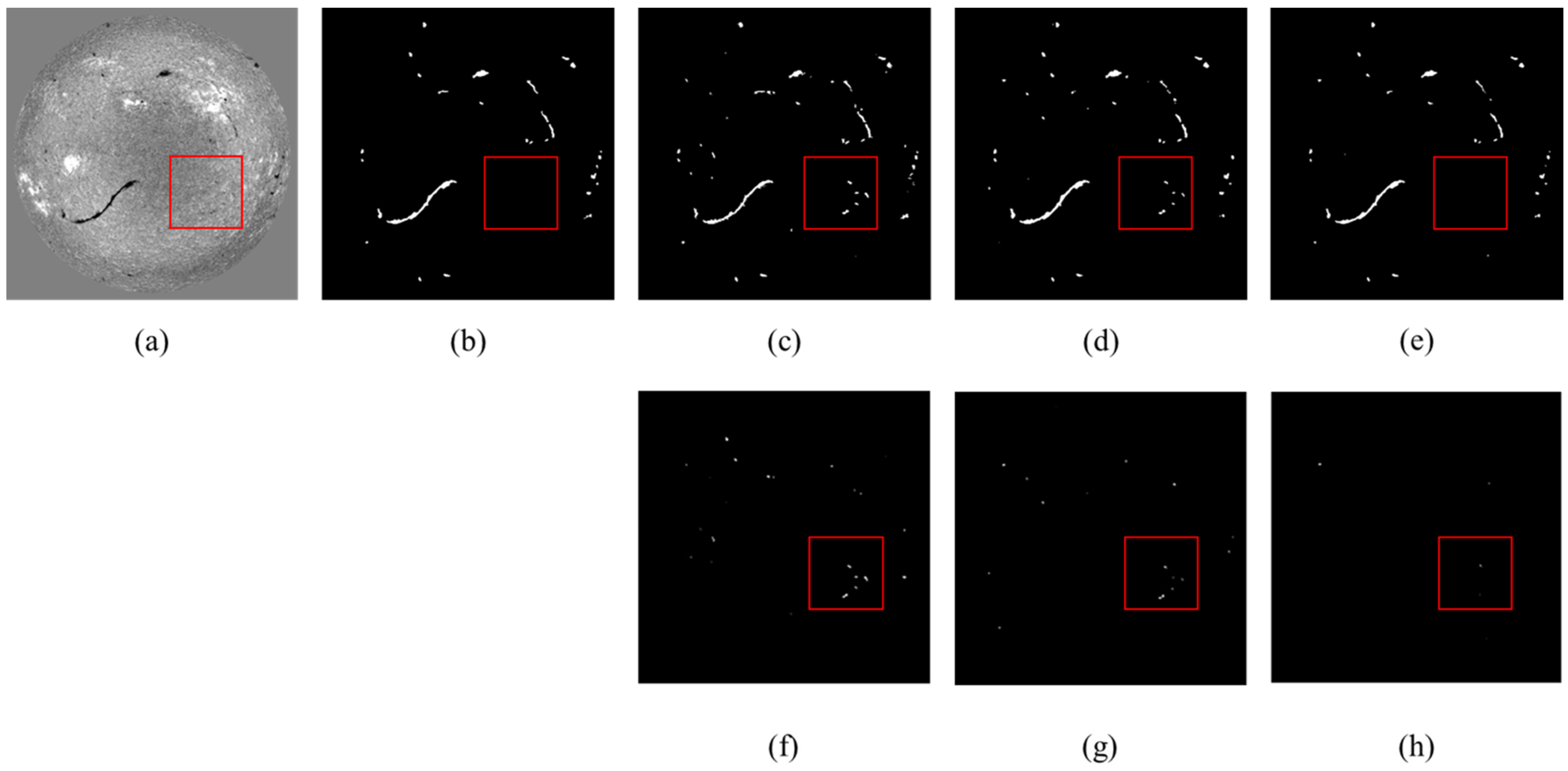
Figure 14 presents another detection case, in which the main factor affecting the detection results is the interference from sunspots. The red box in the figure indicates a sunspot, which should not be detected as a solar filament. The improved U-Net and improved V-Net methods failed to accurately identify the characteristics of the sunspot and mistakenly detected it as a solar filament, compromising their detection performance. In contrast, our method can effectively recognize the characteristics of sunspots and avoid falsely detecting them as solar filaments, achieving better detection results. Figure 14f–h shows the deviations between the results and annotations, obtained through the previously mentioned program. The method exhibits fewer deviation regions.
It can be seen that existing methods have poor anti-interference ability, leading to errors in the results. They have difficulties in dealing with sunspots and background interference. The method proposed in this article achieves better results by better resisting interference. It can better handle images with sunspots and background interference.
6. Conclusions
In the field of filament detection, existing methods face issues such as unreliable dataset annotations and poor anti-interference capability. The work described in this article addresses the above issues. To address the problem of unreliable dataset annotations, this paper manually creates a new solar filament dataset with reduced mislabeling. To tackle the issues of interference, this paper proposes a hybrid CNN-Transformer detection model. Specifically, introducing Transformer can enhance the model’s ability to counter interference. MRB is designed to address the wide range of solar filament sizes. Using deformable large kernel attention and a res path ensures the full integration of encoder and decoder information. Our proposed model can be used to detect solar filaments in full-disk Hα solar images observed by BBSO, outputting the result images with filament annotations.
Compared to existing methods, the detection results of the proposed method show significant improvements in both quantitative and qualitative evaluations. In particular, the improvement is significant for images with sunspots and background interference.
Although this method represents some progress, there are still some issues and limitations. When using this method, it is necessary to preprocess the observed images, which can increase the workload. Future work will include providing a convenient preprocessing program. Due to the introduction of Transformer and improvement modules, a large number of preset parameters, such as the number of Transformer layers and the size of the Patch Embedding block, are introduced during network training. Future work will include conducting more detailed parameter design and ablation experiments to investigate the optimal parameter settings for achieving the best experimental results. The current dataset contains a limited number of images. Future work will focus on studying how to train an efficient detection model with a small number of images, as well as expanding the scale and quantity of the dataset.
Author Contributions
Z.S.: Conceptualization; formal analysis; funding acquisition; investigation; writing—review and editing. M.S.: Conceptualization; formal analysis; investigation; methodology; validation; writing—original draft; writing—review and editing. R.L.: Conceptualization; formal analysis; investigation; writing—review and editing. All authors have read and agreed to the published version of the manuscript.
Funding
This research was funded by the National Natural Science Foundation of China, grant number 12063002.
Data Availability Statement
The Hα image data used to support the findings of this study are observed by the Big Bear Solar Observatory. Image data files we used were downloaded from https://bbsoweb.bbso.njit.edu/pub/archive (accessed on 25 December 2023). The training set and test set data of this study are available from the corresponding author upon request.
Conflicts of Interest
The authors declare no conflicts of interest.
References
- Lin, Y.; Engvold, O.; van der Voort, L.R.; Wiik, J.E.; Berger, T.E. Thin threads of solar filaments. Sol. Phys. 2005, 226, 239–254. [Google Scholar] [CrossRef]
- Martin, S.F. Conditions for the formation and maintenance of filaments—(Invited Review). Sol. Phys. 1998, 182, 107–137. [Google Scholar] [CrossRef]
- Joselyn, J.A.; McIntosh, P.S. Disappearing solar filaments: A useful predictor of geomagnetic activity. J. Geophys. Res. Space Phys. 1981, 86, 4555–4564. [Google Scholar] [CrossRef]
- McCauley, P.I.; Su, Y.; Schanche, N.; Evans, K.E.; Su, C.; McKillop, S.; Reeves, K.K. Prominence and filament eruptions observed by the solar dynamics observatory: Statistical properties, kinematics, and online catalog. Sol. Phys. 2015, 290, 1703–1740. [Google Scholar] [CrossRef]
- Allen, C. Relation between magnetic storms and solar activity. Mon. Not. R. Astron. Soc. 1944, 104, 13–21. [Google Scholar] [CrossRef]
- Chen, H.D.; Zhao, S.Q.; Li, Q.Y.; Jiang, Y.C. The study of filament eruption and its relative phenomena within the solar active region AR0442. Astron. Res. Technol. 2004, 1, 259–267. [Google Scholar] [CrossRef]
- Mackay, D.H.; Karpen, J.T.; Ballester, J.L.; Schmieder, B.; Aulanier, G. Physics of Solar Prominences: II—Magnetic Structure and Dynamics. Space Sci. Rev. 2010, 151, 333–399. [Google Scholar] [CrossRef]
- McIntosh, P.S. Solar magnetic fields derived from hydrogen alpha filtergrams. Rev. Geophys. 1972, 10, 837–846. [Google Scholar] [CrossRef]
- Mouradian, Z.; Soru-Escaut, I. A new analysis of the butterfly diagram for solar filaments. Astronomy 1994, 290, 279–284. [Google Scholar]
- Hanaoka, Y.; Sakurai, T. Statistical study of the magnetic field orientation in solar filaments. Astrophys. J. 2017, 851, 130. [Google Scholar] [CrossRef]
- Gao, J.; Zhou, M.; Wang, H. A Threshold and Region Growing Combined Method for Filament Disappearance Area Detection in Solar Images. In Proceedings of the 35th Annual Conference on Information Sciences and Systems v.1, Baltimore, MD, USA, 21–23 March 2001; pp. 307–311. [Google Scholar]
- Gao, J.; Wang, H.; Zhou, M. Development of an Automatic Filament Disappearance Detection System. Sol. Phys. 2002, 205, 93–103. [Google Scholar] [CrossRef]
- Fuller, N.; Aboudarham, J. Automatic Detection of Solar Filaments Versus Manual Digitization. In Proceedings of the Knowledge-Based Intelligent Information and Engineering Systems(KES 2004) pt.3, Wellington, New Zealand, 20–25 September 2004; pp. 467–475. [Google Scholar]
- Fuller, N.; Aboudarham, J.; Bentley, R.D. Filament recognition and image cleaning on Meudon Hα spectroheliograms. Sol. Phys. 2005, 227, 61–73. [Google Scholar] [CrossRef]
- Shih, F.Y.; Kowalski, A.J. Automatic Extraction of Filaments in Hα Solar Images. Sol. Phys. 2003, 218, 99–122. [Google Scholar] [CrossRef]
- Qu, M.; Shih, F.Y.; Jing, J.; Wang, H. Automatic solar filament detection using image processing techniques. Sol. Phys. 2005, 228, 119–135. [Google Scholar] [CrossRef]
- Zharkova, V.V.; Schetinin, V. Filament recognition in solar images with the neural network technique. Sol. Phys. 2005, 228, 137–148. [Google Scholar] [CrossRef]
- Zharkova, V.V.; Schetinin, V. A Neural-Network Technique for Recognition of Filaments in Solar Images. In Proceedings of the Knowledge-Based Intelligent Information and Engineering Systems, Oxford, UK, 3–5 September 2003; pp. 148–154. [Google Scholar]
- Zhu, J.; Yang, Y.; Su, J.; Liu, H.; Li, X.; Liang, B.; Feng, S. A detection and tracking method for active regions based on deep learning. Astron. Res. Technol. 2020, 17, 191–200. [Google Scholar]
- Li, W.; Zhang, L.; Wu, C.; Cui, Z.; Niu, C. A new lightweight deep neural network for surface scratch detection. Int. J. Adv. Manuf. Technol. 2022, 123, 1999–2015. [Google Scholar] [CrossRef] [PubMed]
- Cui, S.; Xu, Y.; Su, L.; Cui, C.; Fan, D.; Han, J.; Wang, C.; Zhang, L.; Zhang, J. Classification of all-sky camera data based on convolutional neural network. Astron. Res. Technol. 2019, 16, 225–235. [Google Scholar]
- Salasa, R.P.; Arymurthy, A.M. Solar Filament Detection using Mask R-CNN. In Proceedings of the 2019 International Workshop on Big Data and Information Security: IWBIS 2019, Bali, Indonesia, 11 October 2019; IEEE: Bali, Indonesia, 2019; pp. 67–71. [Google Scholar]
- Zhu, G.; Lin, G.; Wang, D.; Liu, S.; Yang, X. Solar Filament Recognition Based on Deep Learning. Sol. Phys. 2019, 294, 117. [Google Scholar] [CrossRef]
- Zehuan, X.; Zhenhong, S. Solar Filament Recognition Based on Improved VNet. Astron. Res. Technol. 2022, 19, 54–64. [Google Scholar] [CrossRef]
- Guo, X.; Yang, Y.; Feng, S.; Bai, X.; Liang, B.; Dai, W. Solar-Filament Detection and Classification Based on Deep Learning. Sol. Phys. 2022, 297, 104. [Google Scholar] [CrossRef]
- Alina, D.; Shomanov, A.; Baimukhametova, S. MaLeFiSenta: Machine Learning for FilamentS Identification and orientation in the ISM. IEEE Access 2022, 10, 74472–74482. [Google Scholar] [CrossRef]
- Vaswani, A.; Shazeer, N.; Parmar, N.; Uszkoreit, J.; Jones, L.; Gomez, A.N.; Kaiser, Ł.; Polosukhin, I. Attention is all you need. Adv. Neural Inf. Process. Syst. 2017, 30, 6000–6010. [Google Scholar]
- Dosovitskiy, A.; Beyer, L.; Kolesnikov, A.; Weissenborn, D.; Zhai, X.; Unterthiner, T.; Dehghani, M.; Minderer, M.; Heigold, G.; Gelly, S. An image is worth 16 × 16 words: Transformers for image recognition at scale. arXiv 2020, arXiv:2010.11929. [Google Scholar]
- Zheng, S.; Lu, J.; Zhao, H.; Zhu, X.; Luo, Z.; Wang, Y.; Fu, Y.; Feng, J.; Xiang, T.; Torr, P.H. Rethinking semantic segmentation from a sequence-to-sequence perspective with transformers. In Proceedings of the IEEE/CVF Conference on Computer Vision and Pattern Recognition, Nashville, TN, USA, 20–25 June 2021; pp. 6881–6890. [Google Scholar]
- Chen, J.; Lu, Y.; Yu, Q.; Luo, X.; Adeli, E.; Wang, Y.; Lu, L.; Yuille, A.L.; Zhou, Y. Transunet: Transformers make strong encoders for medical image segmentation. arXiv 2021, arXiv:2102.04306. [Google Scholar]
- Azad, R.; Niggemeier, L.; Hüttemann, M.; Kazerouni, A.; Aghdam, E.K.; Velichko, Y.; Bagci, U.; Merhof, D. Beyond self-attention: Deformable large kernel attention for medical image segmentation. In Proceedings of the IEEE/CVF Winter Conference on Applications of Computer Vision, Waikoloa, HI, USA, 3–8 January 2024; pp. 1287–1297. [Google Scholar]
- Chen, T.; Kornblith, S.; Norouzi, M.; Hinton, G. A simple framework for contrastive learning of visual representations. In Proceedings of the International Conference on Machine Learning, Virtual Event, 13–18 July 2020; pp. 1597–1607. [Google Scholar]
- Guo, M.H.; Lu, C.Z.; Liu, Z.N.; Cheng, M.M.; Hu, S.M. Visual attention network. arXiv 2022, arXiv:2202.09741. [Google Scholar]
- Wang, S.; Ozcan, K.; Sharma, A. Region-based deformable fully convolutional networks for multi-class object detection at signalized traffic intersections: NVIDIA AICity challenge 2017 Track 1. In Proceedings of the 2017 IEEE SmartWorld, Ubiquitous Intelligence & Computing, Advanced & Trusted Computed, Scalable Computing & Communications, Cloud & Big Data Computing, Internet of People and Smart City Innovation (SmartWorld/SCALCOM/UIC/ATC/CBDCom/IOP/SCI), San Francisco, CA, USA, 4–8 August 2017; pp. 1–4. [Google Scholar]
- Ibtehaz, N.; Rahman, M.S. MultiResUNet: Rethinking the U-Net architecture for multimodal biomedical image segmentation. Neural Netw. Off. J. Int. Neural Netw. Soc. 2020, 121, 74–87. [Google Scholar] [CrossRef] [PubMed]
Figure 1.
Annotations of the two datasets. (a,b) full-disk Hα image; (c,d) annotation image; (a,c) are taken from Dataset 1, while (b,d) are taken from Dataset 2. The white boxes indicate sunspots, the yellow boxes indicate background noise, and the red boxes indicate omitted solar filaments.
Figure 1.
Annotations of the two datasets. (a,b) full-disk Hα image; (c,d) annotation image; (a,c) are taken from Dataset 1, while (b,d) are taken from Dataset 2. The white boxes indicate sunspots, the yellow boxes indicate background noise, and the red boxes indicate omitted solar filaments.

Figure 2.
Two different types of images provided by BBSO. Where (a) is an unprocessed image and (b) is a preprocessed image. The images were observed on 8 November 2013, at 18:23:13 UT.
Figure 2.
Two different types of images provided by BBSO. Where (a) is an unprocessed image and (b) is a preprocessed image. The images were observed on 8 November 2013, at 18:23:13 UT.

Figure 3.
Comparison of Images Before and After Preprocessing. On the (left) is the image before preprocessing, and on the (right) is the image after preprocessing.
Figure 3.
Comparison of Images Before and After Preprocessing. On the (left) is the image before preprocessing, and on the (right) is the image after preprocessing.

Figure 4.
A set of full-disk Hα image and corresponding filament annotation. On the (left) is the full-disk Hα image, and on the (right) is the annotation.
Figure 4.
A set of full-disk Hα image and corresponding filament annotation. On the (left) is the full-disk Hα image, and on the (right) is the annotation.

Figure 5.
Structure of the Transformer layer.

Figure 6.
A full-disk Hα image observed on 21 October 2013 at 19:50:25 UT.

Figure 7.
The structure of the detection model.

Figure 8.
The structure of the MRB.

Figure 9.
Structure of the Decoder Block.

Figure 10.
The decomposition of a large kernel convolution. The colored grids represent the location of convolution kernel and the yellow grid means the center point.
Figure 10.
The decomposition of a large kernel convolution. The colored grids represent the location of convolution kernel and the yellow grid means the center point.

Figure 11.
Structure of DLKA.

Figure 12.
Structure of res path.

Figure 13.
Detection results of different algorithms. (a) Full-disk Hα solar image; (b) Solar filament label map; (c) Detection result using improved U-Net; (d) Detection result using improved V-Net; (e) Detection result using this method; (f–h) Deviations between the results and annotations, obtained through the previously mentioned program. There is background noise in the red box.

Figure 14.
Another compilation of the detection results of different algorithms. (a) Full-disk Hα solar image; (b) Solar filament label map; (c) Detection result using improved U-Net; (d) Detection result using improved V-Net; (e) Detection result using our method; (f–h) Deviations between the results and annotations, obtained through the previously mentioned program. There’s a sunspot in the red box.


Table 1.
Detailed structure of the CNN Encoder.
| Group | In Channels | Out Channels | Blocks |
|---|---|---|---|
| Group 1 | 3 | 64 | MRB×1 |
| Group 2 | 64 | 256 | MRB×2 |
| Group 3 | 256 | 512 | MRB×3 |
Table 2.
Experimental results.
| Method | Precision | Recall | F1 Score |
|---|---|---|---|
| Improved U-Net | 86.74% | 89.49% | 88.09% |
| Improved V-Net | 87.14% | 90.83% | 88.65% |
| This method | 91.50% | 90.89% | 91.19% |
Disclaimer/Publisher’s Note: The statements, opinions and data contained in all publications are solely those of the individual author(s) and contributor(s) and not of MDPI and/or the editor(s). MDPI and/or the editor(s) disclaim responsibility for any injury to people or property resulting from any ideas, methods, instructions or products referred to in the content. |
© 2024 by the authors. Licensee MDPI, Basel, Switzerland. This article is an open access article distributed under the terms and conditions of the Creative Commons Attribution (CC BY) license (https://creativecommons.org/licenses/by/4.0/).
Share and Cite
MDPI and ACS Style
Shang, Z.; Song, M.; Li, R. Solar Filament Detection Based on an Improved Deep Learning Model. Appl. Sci. 2024, 14, 3745. https://doi.org/10.3390/app14093745
AMA Style
Shang Z, Song M, Li R. Solar Filament Detection Based on an Improved Deep Learning Model. Applied Sciences. 2024; 14(9):3745. https://doi.org/10.3390/app14093745
Chicago/Turabian StyleShang, Zhenhong, Mingzhao Song, and Runxin Li. 2024. "Solar Filament Detection Based on an Improved Deep Learning Model" Applied Sciences 14, no. 9: 3745. https://doi.org/10.3390/app14093745
Note that from the first issue of 2016, this journal uses article numbers instead of page numbers. See further details here.