
A Novel Cell-Based Adaptive Cartesian Grid Approach for Complex Flow Simulations
by
 ,
,
Canyan Luo
1,2,
Dan Zhou
1,
Shuang Meng
2,
Lin Bi
2,*,
Wenzheng Wang
3,*,
Xianxu Yuan
2 and
Zhigong Tang
2 1
Key Laboratory of Traffic Safety on Track, Ministry of Education, Central South University, Changsha 410075, China
2
State Key Laboratory of Aerodynamics, China Aerodynamics Research and Development Center, Mianyang 621000, China
3
School of Aeronautics and Astronautics, University of Electronic Science and Technology of China, Chengdu 611731, China
*
Authors to whom correspondence should be addressed.
Appl. Sci. 2024, 14(9), 3692; https://doi.org/10.3390/app14093692
Submission received: 10 April 2024
/
Revised: 19 April 2024
/
Accepted: 24 April 2024
/
Published: 26 April 2024
(This article belongs to the Special Issue Recent Advances in Engineering Applications of Computational Fluid Dynamics)
Abstract
:As the need for handling complex geometries in computational fluid dynamics (CFD) grows, efficient and accurate mesh generation techniques become paramount. This study presents an adaptive mesh refinement (AMR) technology based on cell-based Cartesian grids, employing a distance-weighted least squares interpolation for finite difference discretization and utilizing immersed boundary methods for wall boundaries. This facilitates effective management of both transient and steady flow problems. Validation through supersonic flow over a forward-facing step, subsonic flow around a high Reynolds number NHLP airfoil, and supersonic flow past a sphere demonstrated AMR’s efficacy in capturing essential flow characteristics while wisely refining and coarsening meshes, thus optimizing resource utilization without compromising accuracy. Importantly, AMR simplified the capture of complex flows, obviating manual mesh densification and significantly improving the efficiency and reliability of CFD simulations.
1. Introduction
With the widespread application of computational fluid dynamics (CFD) in fields such as rail transport and aerospace engineering, the complexity of geometric shapes that need to be processed has significantly increased [1]. For instance, the addition of pantographs and bogies to high-speed trains is required to assess the flow field around the entire train, which consequently places higher demands on mesh generation technologies [2,3]. Particularly, the distribution of mesh density often depends on the prior estimation of flow characteristics [4], meaning that even seasoned mesh generation engineers may require weeks, if not longer, to create a high-quality mesh for complex geometries. Given the diversity of flow states in engineering problems, customizing mesh configurations for each specific flow state requires a tremendous amount of work [5]. Therefore, NASA has pointed out in its “CFD Vision 2030” that mesh generation and adaptivity continue to represent critical bottlenecks in the CFD workflow [6].
Research into adaptive mesh refinement (AMR) technology can be traced back to the 1980s [7], with capabilities for initial mesh densification based on geometrical shapes before computation, and dynamic refinement during the solution of governing equations based on flow characteristics [8,9]. The quadtree/octree data structure of Cartesian grids naturally fits with AMR, and De Zeeuw [10] was among the first to introduce AMR based on the quadtree/octree structure into Cartesian grids. Furthermore, the favorable orthogonality of the grid facilitates the computation of flow field gradients, making it easier to capture flow features. In summary, AMR technology has been a significant driving force behind the further development of Cartesian grids, leading some scholars to believe that adaptive Cartesian grids may herald the third major breakthrough in CFD [1].
The AMR approaches under the Cartesian grid framework can be categorized into two types: block-based AMR [11] and cell-based AMR [12,13]. Block-based AMR further divides into patch-based and block-structured adaptations [14]. The patch-based method creates regular, arbitrarily oriented rectangular patches, which are superimposed over areas with insufficient grid resolution to enhance the local resolution, first introduced by Berger and Oliger [15]. In this approach, the grid hierarchy consists of nested, overlapping grids of increasingly higher resolution and does not require a tree data structure to describe the connectivity between blocks. Notable software libraries utilizing patch-based AMR methods include Chombo [16], Samrai [17], and Enzo [18], demonstrating solid performance across various simulation domains. Block-structured AMR, initially proposed and developed by Berger [19] and Quirk [20] among others, can be seen as a simplified variant of the patch-based adaptation. Its characteristic feature is that the entire computational domain is divided into multiple non-overlapping blocks with an identical number of grid cells; the subject of refinement is the block itself, with adaptive history information maintained in a quadtree/octree data structure [21]. Global block refinement may lead to local grid over-densification and consequent memory waste. For example, given an enrichment threshold of 0.7 [22], a block would be refined if more than 70% of its cells were marked for refinement, rendering the remaining 30% as inefficiently refined. This raises another issue, namely the efficiency of block partitioning, requiring further research on how to divide the domain to ensure the most effective use of the refinement threshold. Evidently, both patch-based and block-structured adaptations lack overall flexibility and can be resource-intensive [23].
In contrast, the cell-based AMR introduced by Young et al. [24] also utilizes quadtree/octree data structures for storage, selectively refining individual cells during the adaptive process. This method offers greater flexibility in performing localized and independent cell refinement, and more readily allows for control over the size of distributed grid cells. Compared to block-structured AMR, cell-based AMR has advantages such as saving the number of grid cells required and providing a more flexible adaptation process, making it better suited to handling transient flow and fluid-structure interaction problems [25,26]. Although the benefits of this type of AMR are clear, several issues remain unresolved. On one hand, the flexible refinement approach can lead to a more prevalent occurrence of mismatched levels of adjacent grid cells (hanging grids), compromising computational accuracy. Most previous AMR simulation studies have been based on the finite volume method, which requires special treatment at the interfaces of grids of differing sizes. On the other hand, criteria selection for adaptive Cartesian grid methods under varying flow velocities and characteristics, as well as an assessment of the computational efficiency gains and accuracy improvements brought about by cell-based AMR, have not been fully explored.
In this paper, we build upon cell-based AMR technology and employ a distance-weighted least squares interpolation method to implement finite difference discretization. Additionally, we utilize an immersed boundary method near wall boundaries to conveniently accommodate a variety of flow conditions in both transient and steady-state problems. The organization of the paper is as follows: Section 2 describes the adaptive Cartesian grid technique developed herein, including the grid generation process, criteria for flow field adaptation, grid smoothing, and the assignment of new cell values. Section 3 details the numerical methods used, the discretization of governing equations, handling of hanging grids, and the treatment of immersed boundaries. In Section 4, the capabilities of the adaptive Cartesian grid are analyzed and evaluated through inviscid supersonic/subsonic and high Reynolds number test cases. Finally, conclusions are presented in Section 5.
2. Adaptive Cartesian Grid Generation Method
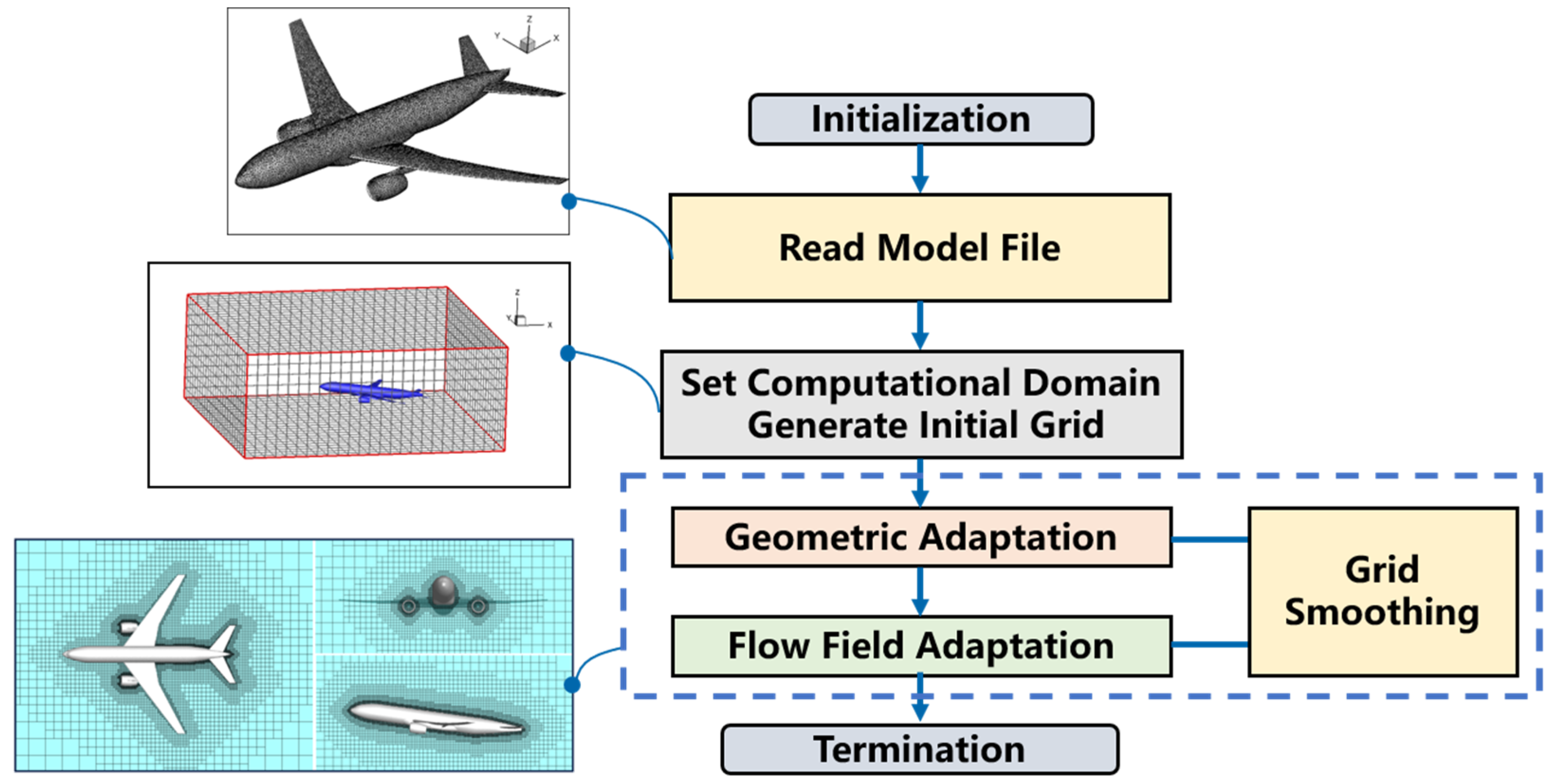
The basic procedure of adaptive Cartesian grid generation is illustrated in Figure 1 as follows: reading in the geometry file; setting the size of the computational domain and generating a uniform initial background grid; identifying different types of grids based on the inside and outside of the geometry and performing geometric adaptation and refinement; during the solving process, incorporating flow features for flow-field adaptation; concurrently, to optimize grid quality during grid adaptation, grid smoothing is also conducted. For detailed implementation of grid generation, please consult references [27,28,29], which cover our team’s advancements in efficient grid generation. The subsequent sections of this paper will concentrate on the adaptive aspects relevant to this study, specifically focusing on the development of an adaptive Cartesian grid method for flow field analysis.
2.1. Initial Uniform Grid Generation
To define the computational domain, only the coordinates of two vertices, and , in floating-point numbers (real) are required. Subsequently, the initial grid numbers in the xyz directions (Nx, Ny, Nz), in integer type, are determined. The mixed arithmetic formula for the grid sizes in the xyz directions (Lx, Ly, Lz) and the initial total number of grids (Ninit) is as follows:
Using integer types to determine the number of grid divisions and subsequently calculating the initial grid sizes facilitates the initial grid partitioning and control of the computational domain size. In contrast, using floating-point types to determine grid sizes and then deriving the number of grids introduces rounding errors due to floating-point truncation. Additionally, considering that the grid sizes in the xyz directions are independent of each other, the initial uniform grid can be established with certain proportions. The determination of computational domain size and the generation of initial uniform grids are illustrated in Figure 2.
2.2. Geometric Adaptation
The dimensions of the edges of the refined sub-cells can be calculated using the integer-type parameter grid level (abbreviated as Lv):
Considering the center coordinates of the father cell , and the center coordinates of the sub-cell , we have:
Firstly, an iterative refinement process is applied to intersecting grids, requiring the pre-setting of the maximum refinement level, Lvmax, in the program. With the increase in refinement levels, the grid’s depiction of the external contour becomes progressively more accurate. For Cartesian grids, the size ratio for grid transition is 2:1, necessitating that the transition speed of the grid not be too rapid. That is, a certain number of grids of the same level must be distributed in one direction. The grids in the transition area are referred to as buffer layers, denoted as Nbl. A reasonable Nbl facilitates the selection of appropriate interpolation templates during the flow field solution process [30], enhancing the accuracy of the computational results. Figure 3 illustrates the process of geometric adaptive grid refinement for the entire DWP aircraft model, including the refinement of intersecting grids and the addition of buffer layers.
2.3. Flow Field Adaptation
Since the initial computational grid is usually adaptively generated based on the geometry of the object, it tends to be denser around the surface of the object and lower in resolution in areas far from the object, making it difficult to accurately reflect complex flow characteristics. Therefore, to capture features such as vortices, shock waves, and shear layers within the flow, it is necessary to dynamically adjust the grid resolution based on the flow field solution, refining the grid where needed to more precisely capture flow characteristics.
First, as referenced in [10,12], it is necessary to compute the velocity divergence di, and vorticity ri, for each cell, incorporating the grid scale:
Here, h denotes the side length of the target grid cell, with k = 2 for two-dimensional and k = 3 for three-dimensional spaces. Upon computing the velocity divergence and vorticity across all N grid cells, the standard deviations for both parameters are:
Herein, Sd and Sr represent the standard deviations of velocity divergence and vorticity, respectively. Ultimately, this determines whether the target grid requires refinement or coarsening:
In this context, r1, r2, and c1, c2 are empirical coefficients that should be specified for specific flow problems, as indicated in references [10,12]. Due to the varying dominant flow features in different flow problems, the coefficients for velocity divergence and vorticity can be adjusted accordingly. Generally speaking, larger coefficient values increase the threshold for grid refinement and decrease the threshold for coarsening, resulting in fewer total grid cells within the computational domain; conversely, smaller values increase the number of adaptive grid cells. This adjustment allows for better adaptation to the requirements of different flow problems, effectively enhancing the accuracy and efficiency of numerical simulations.
2.4. Grid Smoothing
The next step involves grid quality assessment, which typically accompanies the entire process of grid refinement and coarsening throughout the computation (including the initial geometry-based and flow-based adaptive stages) and requires multiple iterative procedures aimed at eliminating any unreasonable grid configurations within the region. As illustrated in Figure 4a, “hole elements” [31] refer to grid cells that are flanked by neighboring cells with sub-cells on either side or top and bottom; and Figure 4b shows the scenario where the grid level difference between adjacent cells exceeds one. To address these issues, it is necessary to inspect the neighbor levels of the target grid in all directions and compare the level differences between the target grid and its neighbors. If the target grid’s level is less than that of grids in multiple directions, or if the level difference with a neighbor exceeds one, then the target grid must be refined. This process involves repeated recursive checks of all grids until all irrational features are eliminated.
2.5. Assignment of Newly Generated Grids
As grid refinement and coarsening progress, newly generated grids are continuously produced. Figure 5 presents two types of these grids (for both refinement and coarsening scenarios). Unlike the geometric adaptivity prior to computation, which only requires assigning location information, topological relationships, and intersection relations to the newly generated grids, the flow-based adaptivity also involves processing the flow field values of the new grids, such as basic flow variables and turbulence quantities. The flow field information of the new grids must first ensure conservation, for example, by employing a simple assignment method. For new grids generated by coarsening, the calculation of the flow field value is as follows:
In the formula, n denotes the number of sub-cells. Specifically, within the isotropic Cartesian grid described in this study, n equals 4 in two dimensions and 8 in three dimensions. Additionally, for newly refined grids, the method to calculate the flow field values is as follows:
To ensure accuracy and local conservation, Zhu and Qiu [32] proposed an L2 projection method for determining the flow field information of newly emerged grid cells. Their research provides a detailed derivation process and analyzes its conservation and accuracy. Here, the final expression with second-order accuracy is given; for example, in two dimensions, for calculating the flow field value of sub-cells in the refinement scenario, the formula is as follows:
wherein , represent the quadrants of the four sub-cells to . and represent the size of cell ; while and signify the gradients of the flow field variable at point . It is apparent that this formulation is easily extendable to three-dimensional scenarios. For the coarsening scenario, the formula for calculating the flow field values of the new grid remains as in Equation (7).
3. Numerical Methods
3.1. Governing Equations
In compressible RANS simulations, Favre-averaged Navier–Stokes equations are used:
where ui, ρ, p, and E are the mean velocity components, the density, the pressure, and the specific internal energy respectively. The Reynolds stress tensor is derived using the Boussinesq approximation:
where μ and μt are the molecular dynamic viscosity and the eddy viscosity, respectively. Furthermore, the heat flux is defined as follows:
where cp is the specific heat at constant pressure and T is the temperature. The laminar Prandtl number Pr is 0.72 and the turbulent Prandtl number Prt is 0.9.
The solver presented in this paper is founded on the finite difference method, with the inviscid terms being discretized through the employment of the Roe approximate Riemann solver in conjunction with a third-order accurate MUSCL scheme. The discretization of viscous terms is achieved via a second-order central difference scheme. For time discretization, an explicit third-order Runge–Kutta scheme is utilized for unsteady problems, whereas steady problems employ the lower-upper symmetric Gauss–Seidel implicit advancement scheme.
3.2. Hanging Grids Discretization
In previous studies [25], Lagrange polynomials were utilized to extend the solution from a coarse to a fine grid level, demonstrating their suitability within the AMR framework. The solvers, which are based on grid-nodal points, essentially perform one-dimensional interpolation exclusively at the hanging nodes. The solver in this study is cell-centered, with center nodes of adjacent cells experiencing coordinate changes in all directions at hanging grids. This paper addresses the discretization challenges posed by hanging nodes through the use of the distance-weighted least squares (DWLS) interpolation method. This approach offers enhanced flexibility in stencil selection, while simultaneously ensuring interpolation accuracy through the development of basis functions. It utilizes adjacent mesh cells surrounding the hanging nodes to construct equidistant finite difference stencils. Following mesh smoothing, adjacent cells are maintained with a level difference not exceeding one. At this juncture, the hanging nodes can be categorized into two types, as depicted in Figure 6.
For the first scenario, regardless of whether bilinear interpolation (or trilinear interpolation within a 3D context involving 8 sub-cells) or inverse distance weighting interpolation is employed, the final outcome can be simplified to:
This interpolated formula exhibits second-order accuracy, where represents the solution variables required by the solver, such as the primitive variables , etc.
The second type of hanging grid, taking discretization in the i+ direction as an example, has its interpolation stencil illustrated in Figure 7, where the required template can be conveniently determined through the neighbors. Subsequently, the linear basis is employed to approximate the target function:
wherein x denotes the position vector, and the corresponding coefficient vector a is determined by minimizing the following objective function , expressed as:
In the equation, the subscript n represents the number of interpolation stencil cells, the subscript R refers to the corresponding target point, represents weight functions indicating the importance of different stencil points, is the diagonal expansion matrix, is the vector of flow field values from the selected interpolation stencil cells, and is the position matrix of the selected stencil cells. When , we have:
By solving this, the coefficient vector a is obtained:
Substituting the coordinates of the target node, its value is determined as:
In three dimensions, the basis is considered, and using the interpolation method presented in this paper allows for the flexible and convenient selection of the surrounding stencils at the hanging grid locations for corresponding expansion.
3.3. Boundary Treatment
The immersed boundary method (IBM) on Cartesian grids demonstrates significant advantages in terms of automation, as it allows for the generation of high-quality computational grids for flow fields without the dependence on physical surface meshes [33,34]. In this paper, we adopted a sharp-interface immersed boundary approach to handle physical surface boundaries. As illustrated in Figure 8, fluid cells were classified and labeled, and local reconstructions were performed near the grid nodes close to the physical surface to enforce immersed boundary conditions (IBC). Such methods are simple in form, easy to implement, and readily integrated with flow solvers [35]. As for the elements used to implement the boundary conditions, they can be located inside the physical surface, known as the ghost cell method [36], or the grid cells near the surface can be modified using wall function theories [37,38]. The implementation of IBC principally includes the following four key aspects: (1) classifying the grid types based on their relative positions to the physical surface; (2) selecting and locating reference points; (3) interpolating at these reference points; and (4) obtaining the physical quantities for ghost/wall-modeled cells based on reference points and boundary conditions. For inviscid flows and flows with low Reynolds numbers, this paper adopted the ghost cell method proposed by Pan [36] to handle physical surface boundary conditions, as shown in Figure 8a. For high Reynolds number wall-bounded turbulent flows, the idea of tangential velocity reconstruction described in references [37,38] was used to modify the grid cells near the wall, as depicted in Figure 8b.
4. Results and Discussion
4.1. A Mach 3 Wind Tunnel with a Forward Facing Step
To verify the capability of the developed cell-based AMR method in capturing flow features such as shock discontinuities and shear layers, the classic Woodward–Colella test [39], namely the forward facing step flow problem, was selected for simulation studies. The computational domain for the step was a rectangular area of L × H = 3.0 × 1.0, with the step height being 0.2, positioned at a distance x = 0.6 from the wind tunnel entrance. The freestream Mach number Ma = 3.0, and supersonic inflow and outflow boundary conditions, were set at the inlet and outlet, respectively, with slip adiabatic solid wall boundary conditions applied to both the upper and lower boundaries. The initial grid generation is illustrated in Figure 9, where the initial cell size Δx = Δy = 0.05, with a maximum of three layers of refinement, and the initial number of grid cells being 11,397.
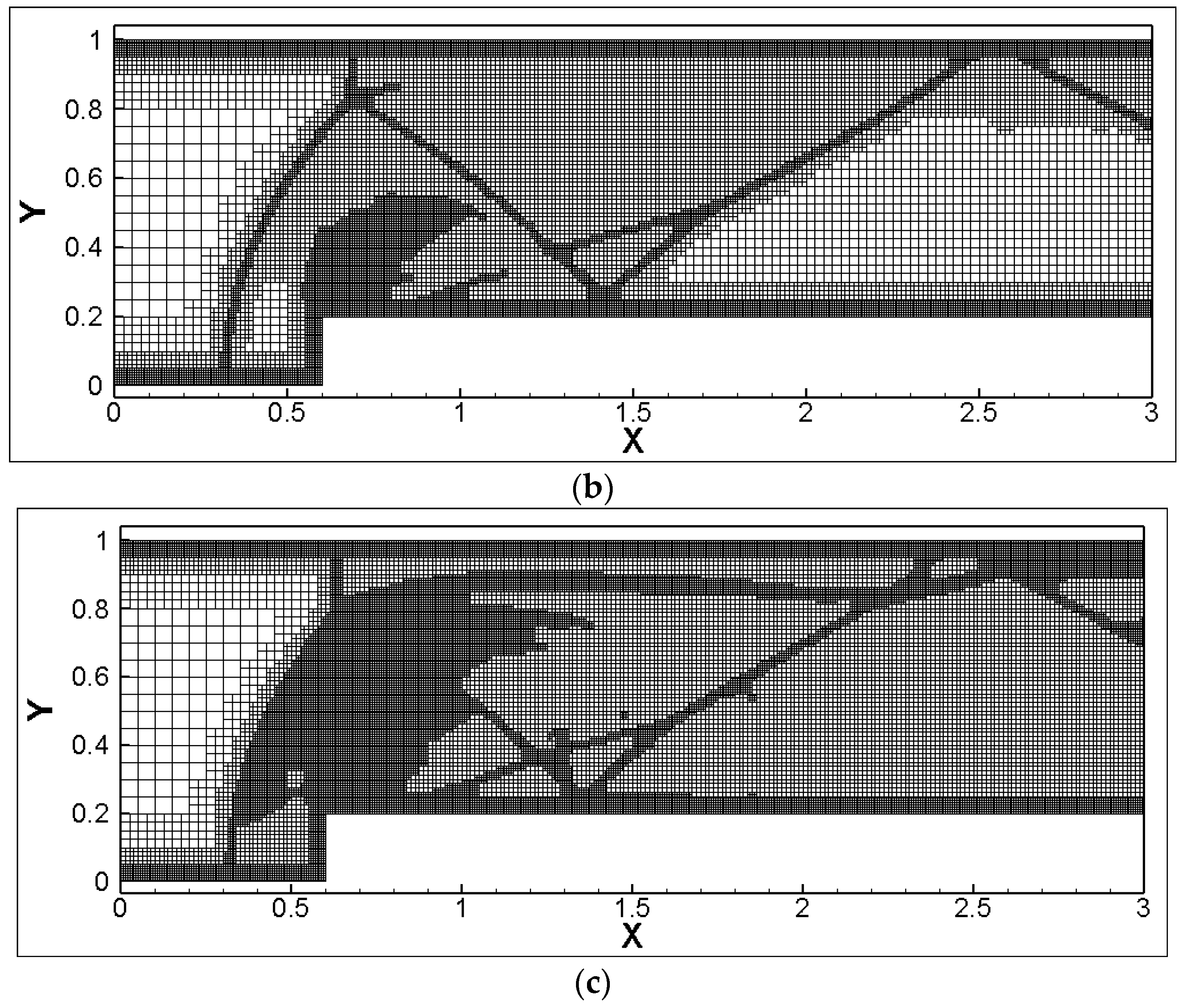
Based on three adaptive criteria (velocity vorticity-based, velocity divergence-based, and a combined criterion of velocity vorticity divergence), the grid distribution at the time instant (t* = tMa∞/H = 4) is shown in Figure 10, with the grid numbers being 22,668, 22,092, and 31,617, respectively. At this moment, the flow details within the region include: (1) three times shock reflection and their paths; (2) expansion waves at the step corner and the weak oblique shock waves induced by its upper surface; (3) minor oscillations in entropy behind the Mach stem directly above the step, followed by the vortex roll-up (Kelvin–Helmholtz instability). It was observed that the velocity vorticity criterion could capture the details of shear layers and vortices in the flow field relatively well, but was weak in capturing shock discontinuities. On the other hand, the velocity divergence criterion had a strong capability in capturing shocks but failed to accurately capture shear layers. The combined criterion of velocity vorticity-divergence was able to more comprehensively capture the flow field features under complex scenarios.
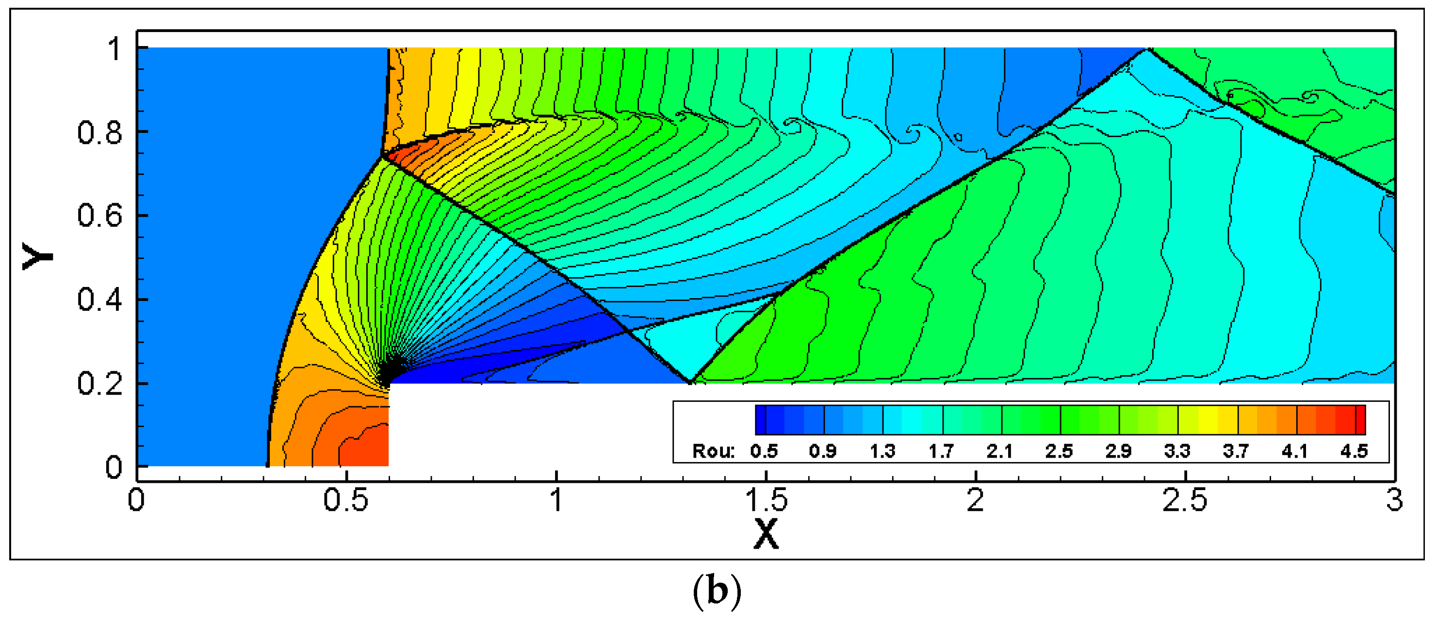
To compare the effect of different numbers of adaptive refinement layers on the solution efficiency, an additional two layers of adaptation were introduced under the prior background mesh size, thus considering a flow field solution adaptation with five layers. Figure 11 displays the flow field distribution under the five-layer solution adaptation. It is evident, compared to the previous section, that the shock width was narrower, and more refined vortex roll-ups were captured behind the Mach stem.
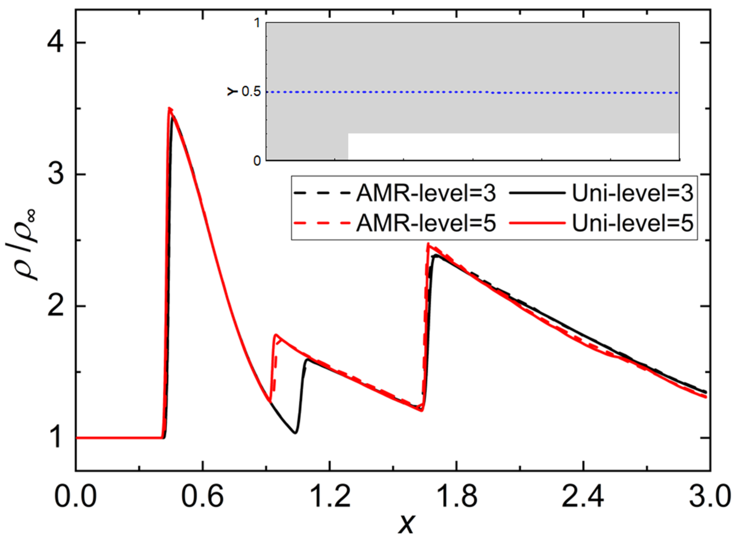
To compare the impact of AMR on the spatial distribution of the flow field, Figure 12 presents the density distribution along the midline at y = 0.5 of the step height at the aforementioned time instant. The label “Uni” denotes the uniform grid discretization solution using the finest mesh size corresponding to the areas of interest. As can be discerned from the figure, activating AMR had a minimal effect on the flow field results, achieving an outcome comparable to the simulation with a uniformly fine mesh.
In this test case, the comparison of the dimensionless computational expense between cell-based AMR grids and uniform grids is shown in Table 1. Under the uniform grid, the compute time was approximately proportional to the total number of cells (a quarter-scale reduction results in a sixteen-fold increase in the overall number of cells). Regarding the computational time for the AMR setup, considering the evolving and unsteady nature of the flow within the computational domain, the AMR strategy dynamically refined the mesh in regions with steep flow gradients and coarsened it in areas with smoother flow. The table serves as a point of reference, listing the number of grids at the moments previously discussed. Overall, AMR efficiently captured flow details and achieved a significant reduction in computational costs. As indicated by the results in the table, with three layers of solution adaptivity, the number of cells at the final time step and the overall computational expense were reduced to 48.9% and 47.6% of those for the uniform grid; when the level of adaptivity was elevated to five layers, these ratios further decreased to 15.8% and 19.5%, respectively. This demonstrates that increasing the number of solution adaptation layers significantly enhanced the efficiency of the simulation.
4.2. Subsonic NHLP Airfoil
The NHLP three-element airfoil was composed of a leading-edge slat, main wing, and trailing-edge flap. The deflection angle of the leading-edge slat for the NHLP airfoil was set at 25°, and the trailing-edge flap was deflected at 20°. Extensive testing of this airfoil was conducted in the British Aircraft Corporation (BAC) wind tunnel [40]. The selected test conditions were as follows: the incoming flow Mach number was 0.197, the angle of attack 4.01°, and the Reynolds number 3.52 × 10⁶.
The intricate geometries, such as narrow gaps between different wing sections and complex surface features like cutouts, posed significant challenges for the topology design, mesh point distribution, and mesh quality control of body-fitted structured grids; however, the immersed boundary adaptive Cartesian grid method enabled the rapid generation of high-quality computational meshes. The computational domain was set to [−16, 25] × [−20, 20] with the initial Cartesian grid size of Δy = Δx = 1.28. The maximum refinement level was set to 12 layers with 7 buffer layers. The final geometry-adaptive grid, as shown in Figure 13, consisted of approximately 1.51 × 10⁵ cells and was generated in just 8.6 s on a desktop computer under single-core conditions. Near-wall treatment was applied using the wall function approach, with the SA turbulence model implemented. Reference points at the same distance were considered near the wall, with an overall average y+ of around 300. The simulation employed the LU-SGS scheme for progression and initiated AMR after the flow field reached preliminary stability.
The grid layout before and after AMR is illustrated in Figure 14. The figure reveals that the adaptive criterion refined the wake region to better capture the flow characteristics in that area.
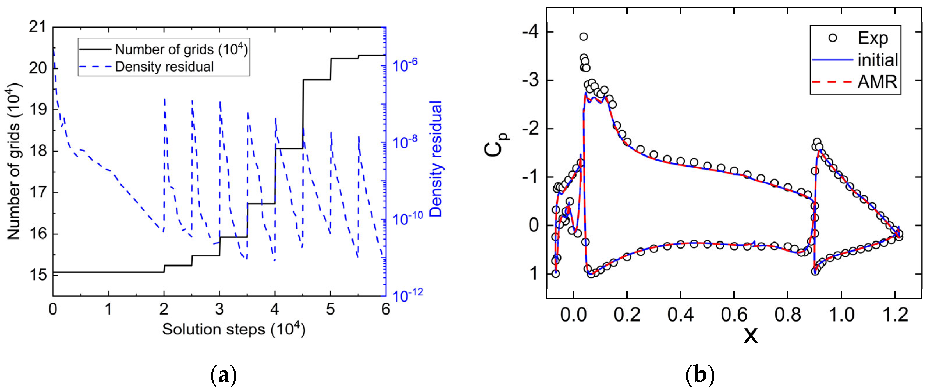
Figure 15a presents the curve showing the change in the number of grids during the AMR process, as well as the convergence curve for the density residuals. After eight AMR iterations, the number of grids increased from 1.51 × 10⁵ to 2.03 × 10⁵. The change in grid numbers was relatively small in the last AMR iteration, and the residuals also further converged, indicating that both the flow field and the grid had been sufficiently developed. Figure 15b displays the surface pressure coefficient curves before and after AMR. Due to the use of the wall function model in this study, errors were inevitably present in areas of flow separation, such as at the leading edges of the slat and the main wing. Moreover, with the mesh involving 8 layers of grids for AMR and 12 layers for the mesh near the wing surface, activating adaptation did not alter the mesh distribution near the wall, thus having a minimal impact on surface quantities. When we selected the maximum Cp values for the leading edges of the slat, main wing, and tail wing, which were less influenced by flow separation, the discrepancies between the findings of this study and the experimental results were −1.9%, 0.1%, and 4.1%, respectively. Additionally, the magnitude of error was very similar, regardless of whether AMR was activated or not. However, the primary effect of AMR was to significantly enhance the resolution in the wake region.
Figure 16 and Figure 17 present the flow field and the turbulent viscosity coefficient contours around the airfoil before and after AMR. The figures indicate that the velocity magnitude in the wake region decreased after AMR, corresponding to an increase in the turbulent viscosity coefficient. The cell-based AMR technique significantly improved the simulation accuracy in the wake region by adaptively increasing the grid resolution.
4.3. Supersonic Flow around a Sphere
The sphere had a diameter of D = 2, with an incoming flow Ma of 1.9 and a Reynolds number based on the diameter (ReD) of 1 × 10⁵. The computational domain was set to 30 × 40 × 40, as shown in Figure 18a. The initial Cartesian grid size was Δy = Δx = 2.0, with an initial grid count of 6000. A maximum of 8 levels of refinement was set, resulting in a final adaptive mesh counting 5.3 million cells for the flow field. Figure 18b illustrates the space-filling Cartesian grid around the sphere and the triangular mesh on the surface of the sphere, with the sphere surface discretized into 10,278 triangular elements.
Figure 19 presents the grid before flow AMR and the corresponding Mach number contours, demonstrating that after 1000 steps of evolution, the detached shock in front of the sphere started to emerge. However, due to insufficient grid resolution in regions far from the surface, the flow field features could not be accurately described. With the continuous process of adaptation, the characteristics of the flow field became more pronounced, and shock capturing became finer. By the time of the sixth solution adaptation, the criteria for solution adaptation had effectively captured the bow shock in front of the sphere as well as the expansion shock generated at the rear, indicating that the flow field had been sufficiently developed.
Figure 20 illustrates the impact of AMR on the pressure coefficient distribution over the surface of the sphere. The figure reveals that, with the given number of surface triangular mesh elements, a smooth representation of surface quantities could be extracted from the Cartesian grid of the flow field for subsequent force integration processing. Additionally, the AMR had a minor effect on the pressure distribution in the stagnation region ahead of the flow but had a more significant impact on the separated region at the rear. When calculated on a coarser grid, the negative pressure region’s amplitude and extent at the back were overestimated, affecting the overall drag coefficient. In Table 2, upon comparing the simulation results of this study with the experimental results of Bailey and Hiatt [41], it is evident that thanks to the finer resolution in the wake achieved by the AMR (increasing the overall grid count from 1.38 million to 4.17 million), the overall drag coefficient was brought closer to the experimental values.
5. Conclusions
This research developed a technique based on cell-based AMR Cartesian grids. It utilized a DWSL method for the discretization of the finite difference method and adopted IBMs near physical boundaries. This approach facilitated the handling of both transient and steady flow problems under various velocity conditions flexibly and conveniently. Based on the analysis conducted, the following conclusions are drawn:
- In the context of supersonic flow over a forward facing step, employing a comprehensive criterion based on velocity, vorticity, and divergence enhanced the capture of flow field characteristics. AMR achieved comparable flow field results to uniform grids, while judicious grid coarsening and refinement reduced computational costs without compromising simulation accuracy. With solution adaptation across three layers, grid count and overall computational cost decreased to 48.9% and 47.6%, respectively, compared to uniform fine grids. Increasing adaptation layers to five further reduced these ratios to 15.8% and 19.5%, respectively.
- In the simulation of a high Reynolds number turbulent flow over an NHLP three-element airfoil, the immersed Cartesian grid method autonomously generated the required computational grid within seconds. After eight iterations of AMR, the number of grids increased from 1.51 × 10⁵ to 2.03 × 10⁵. While activating AMR had a minor effect on surface pressure coefficients, it significantly enhanced the resolution of the simulation in the wake region.
- For the three-dimensional supersonic flow simulation around a sphere, the initial grid resolution was inadequate for accurately portraying the features of the flow field. Through six iterations of solution adaptation, the accuracy in capturing shock waves was significantly improved, particularly at the front and rear of the sphere. Although this process had a minimal impact on the pressure distribution in the stagnation region, it notably improved the prediction of the separation zone, avoiding the overestimation of negative pressure regions, and thus, making the predictions of drag coefficients closer to experimental results.
In the future, our research endeavors will focus on pioneering higher-order numerical algorithms and efficient parallel technologies. These advancements aim to enhance simulation accuracy, reduce computational costs, and ultimately address the escalating demands posed by increasingly complex and larger-scale engineering problems.
Author Contributions
Conceptualization, X.Y. and Z.T.; methodology, C.L. and L.B.; formal analysis, C.L., D.Z. and W.W.; investigation, S.M. and W.W.; writing—original draft preparation, C.L. and S.M.; writing—review and editing, C.L., D.Z. and L.B.; supervision, X.Y. and Z.T.; funding acquisition, L.B. and C.L. All authors have read and agreed to the published version of the manuscript.
Funding
This research was funded by National Key Research and Development Program of China (Grant No. 2019YFA0405204) and the Postgraduate Scientific Research Innovation Project of Hunan Province (Grant No. CX20230237).
Institutional Review Board Statement
Not applicable.
Informed Consent Statement
Not applicable.
Data Availability Statement
The data presented in this study are available in the article.
Conflicts of Interest
The authors declare no conflict of interest.
References
- Nakahashi, K. Aeronautical CFD in the age of Petaflops-scale computing: From unstructured to Cartesian meshes. Eur. J. Mech. B 2013, 40, 75–86. [Google Scholar] [CrossRef]
- Meng, S.; Li, X.; Chen, G.; Chen, Z. Numerical simulation of slipstreams and wake flows of trains with different nose lengths passing through a tunnel. Tunn. Undergr. Space Technol. 2020, 108, 103701. [Google Scholar] [CrossRef]
- Ji, P.; Wu, F.; Qian, B.; Yan, L. Aerodynamic Shape Design of Pantograph Network Monitoring Device on High-Speed Trains. J. Appl. Fluid Mech. 2019, 12, 1383–1394. [Google Scholar] [CrossRef]
- Baker, T.J. Mesh generation: Art or science. Prog. Aerosp. Sci. 2005, 41, 29–63. [Google Scholar] [CrossRef]
- Larsson, J.; Wang, Q. The Prospect of Using Large Eddy and Detached Eddy Simulations in Engineering Design, and the Research Required to Get There. Philos. Trans. R. Soc. A Math. Phys. Eng. Sci. 2014, 372, 20130329. [Google Scholar] [CrossRef]
- Slotnick, J.; Khodadoust, A.; Alonso, J.; Darmofal, D.; Gropp, W.; Lurie, E.; Mavriplis, D. CFD Vision 2030 Study: A Path to Revolutionary Computational Aerosciences; NASA/CR-2014-218178; NASA Technical Reports Server; NASA: Hampton, VI, USA, 2014.
- Thompson, J.F. A survey of dynamically-adaptive grids in the numerical solution of partial differential equations. Appl. Numer. Math. 1985, 1, 3–27. [Google Scholar] [CrossRef]
- Lourenço, M.A.; Padilla, E.L. An octree structured finite volume based solver. Appl. Math. Comput. 2020, 365, 1–28. [Google Scholar] [CrossRef]
- Cant, R.S.; Ahmed, U.; Fang, J.; Chakarborty, N.; Nivarti, G.; Moulinec, C.; Emerson, D.R. An unstructured adaptive mesh refinement approach for computational fluid dynamics of reacting flows. J. Comput. Phys. 2022, 468, 111480. [Google Scholar] [CrossRef]
- Zeeuw, D.L.D. A Quadtree-Based Adaptively-Refined Cartesian-Grid Algorithm for Solution of the Euler Equations; University of Michigan: Ann Arbor, MI, USA, 1993. [Google Scholar]
- Dubey, A.; Almgren, A.; Bell, J.; Berzins, M.; Brandt, S.; Bryan, G.; Colella, P.; Graves, D.; Lijewski, M.; Löffler, F.; et al. A survey of high level frameworks in block-structured adaptive mesh refinement packages. J. Parallel Distrib. Comput. 2014, 74, 3217–3227. [Google Scholar] [CrossRef]
- Jahangirian, A.; Shoraka, Y. Adaptive unstructured grid generation for engineering computation of aerodynamic flows. Math. Comput. Simulat. 2008, 78, 627–644. [Google Scholar] [CrossRef]
- Xu, W.; Li, K.; Geng, Z.; Zhang, M.; Yang, J. A Local Adaptive Mesh Refinement for JFO Cavitation Model on Cartesian Meshes. Appl. Sci. 2021, 11, 9879. [Google Scholar] [CrossRef]
- Freret, L.; Williamschen, M.; Groth, C.P.T. Enhanced anisotropic block-based adaptive mesh refinement for three-dimensional inviscid and viscous compressible flows. J. Comput. Phys. 2022, 458, 111092. [Google Scholar] [CrossRef]
- Berger, M.J.; Oliger, J. Adaptive mesh refinement for hyperbolic partial differential equations. J. Comput. Phys. 1984, 53, 484–512. [Google Scholar] [CrossRef]
- Adams, M.; Colella, P.; Graves, D.T.; Ligocki, T.J.; Martin, D.F.; Straalen, B.V. Chombo Software Package for AMR Applications-Design Document; Technical Report LBNL-6616E; Lawrence Berkeley National Laboratory: Berkeley, CA, USA, 2015. Available online: https://commons.lbl.gov/display/chombo/Chombo+-+Software+for+Adaptive+Solutions+of+Partial+Differential+Equations (accessed on 9 April 2024).
- Wissink, A.M.; Hornung, R.D.; Kohn, S.R.; Smith, S.S.; Elliott, N. Large Scale Parallel Structured AMR Calculations Using the SAMRAI Framework. In Proceedings of the 2001 ACM/IEEE Conference on Supercomputing, Denver, CO, USA, 10–16 November 2001; Available online: https://computing.llnl.gov/projects/samrai (accessed on 9 April 2024).
- O’Shea, B.W.; Bryan, G.; Bordner, J.; Norman, M.L.; Kritsuk, A. Introducing Enzo, an AMR Cosmology Application; Springer: Berlin/Heidelberg, Germany, 2005; pp. 341–349. Available online: https://enzo.readthedocs.io/en/latest/index.html (accessed on 9 April 2024).
- Berger, M.J.; Saltzman, J.S. AMR on the CM-2. Appl. Numer. Math. 1992, 14, 239–253. [Google Scholar] [CrossRef]
- Quirk, J.J.; Hanebutte, U.R. A Parallel Adaptive Mesh Refinement Algorithm; ICASE: Hampton, VI, USA, 1993; pp. 63–93. [Google Scholar]
- Fakhari, A.; Lee, T. Finite-difference lattice Boltzmann method with a block-structured adaptive-mesh-refinement technique. Phys. Rev. E Stat. Nonlinear Soft Matter Phys. 2014, 89, 33310. [Google Scholar] [CrossRef]
- Maeyama, H.; Imamura, T.; Osaka, J.; Kurimoto, N. Unsteady aerodynamic simulations by the lattice Boltzmann method with near-wall modeling on hierarchical Cartesian grids. Comput. Fluids. 2022, 233, 105249. [Google Scholar] [CrossRef]
- Ishida, T.; Takashi, S.; Nakahashi, K. Efficient and Robust Cartesian Mesh Generation for Building-Cube Method. J. Comput. Sci. Technol. 2008, 2, 435–446. [Google Scholar] [CrossRef]
- Young, D.P.; Melvin, R.G.; Bieterman, M.B.; Johnson, F.T.; Samant, S.S.; Bussoletti, J.E. A locally refined rectangular grid finite element method: Application to computational fluid dynamics and computational physics. J. Comput. Phys. 1991, 92, 1–66. [Google Scholar] [CrossRef]
- Wang, Z.; Du, L.; Sun, X. Adaptive mesh refinement for simulating fluid-structure interaction using a sharp interface immersed boundary method. Int. J. Numer. Methods Fluids 2020, 92, 1890. [Google Scholar] [CrossRef]
- Choung, H.; Saravanan, V.; Lee, S. Cell-based hybrid adaptive mesh refinement algorithm for immersed boundary method. Int. J. Numer. Methods Fluids. 2022, 94, 272–294. [Google Scholar]
- Meng, S.; Zhou, D.; Yuan, X.X.; Li, X.L.; Chen, H.; Bi, L. Enhanced strategy for adaptive Cartesian grid generation with arbitrarily complex 3D geometry. Adv. Eng. Softw. 2022, 174, 103304. [Google Scholar] [CrossRef]
- Meng, S.; Zhou, D.; Bi, L.; Li, X.L.; Luo, C.Y.; Du, H. Anisotropic Cartesian grid generation strategy for arbitrarily complex geometry based on a fully threaded tree. Comput. Aided Des. 2023, 155, 103447. [Google Scholar] [CrossRef]
- Li, X.L.; Yang, M.Z.; Bi, L.; Xu, R.; Luo, C.Y.; Yuan, S.; Yuan, X.; Tang, Z.G. An efficient Cartesian mesh generation strategy for complex geometries. Comp. Methods Appl. Mech. Eng. 2024, 418, 116564. [Google Scholar] [CrossRef]
- Tang, Z.G.; Chen, H.; Bi, L.; Yuan, X. Numerical simulation of supersonic viscous flow based on adaptive Cartesian grid. Acta Aeronaut. Astronaut. Sin. 2018, 39, 44–56. (In Chinese) [Google Scholar]
- Linde, T.; Roe, P.L. An adaptive Cartesian mesh algorithm for the Euler equations in arbitrary geometries. In Proceedings of the 9th Computational Fluid Dynamics Conference, Buffalo, NY, USA, 13–15 June 1989; pp. 89–1930. [Google Scholar]
- Zhu, H.; Qiu, J. An h-adaptive RKDG method with troubled-cell indicator for two-dimensional hyperbolic conservation laws. Adv. Comput. Math. 2013, 39, 445–463. [Google Scholar] [CrossRef]
- Zeng, Y.; Wang, Y.; Yang, D.; Chen, Q. Immersed Boundary Methods for Simulations of Biological Flows in Swimming and Flying Bio-Locomotion: A Review. Appl. Sci. 2023, 13, 4208. [Google Scholar] [CrossRef]
- Verzicco, R. Immersed boundary methods: Historical perspective and future outlook. Annu. Rev. Fluid Mech. 2023, 55, 129–155. [Google Scholar] [CrossRef]
- Forrer, H.; Jeltsch, R. A higher order boundary treatment for Cartesian-grid methods. J. Comput. Phys. 1998, 140, 259–277. [Google Scholar] [CrossRef]
- Pan, D. A General Boundary Condition Treatment in Immersed Boundary Methods for Incompressible Navier-Stokes Equations with Heat Transfer. Numer. Heat Transf. Part B Fundam. 2012, 61, 279–297. [Google Scholar] [CrossRef]
- Tamaki, Y.; Harada, M.; Imamura, T. Near-wall modification of Spalart–Allmaras turbulence model for immersed boundary method. AIAA J. 2017, 55, 3027–3039. [Google Scholar] [CrossRef]
- Constant, B.; Péron, S.; Beaugendre, H.; Benoit, C. An improved immersed boundary method for turbulent flow simulations on Cartesian grids. J. Comput. Phys. 2021, 435, 110240. [Google Scholar] [CrossRef]
- Woodward, P.; Colella, P. The numerical simulation of two-dimensional fluid flow with strong shocks. J. Comput. Phys. 1984, 54, 115–173. [Google Scholar] [CrossRef]
- AGARD-AR-303; Measurements on a Two-Dimensional Airfoil with High Lift Devices: A Selection of Experimental Test Cases for the Validation of CFD Codes. NATO: Brussels, Belgium, 1994.
- Bailey, A.B.; Hiatt, J. Sphere Drag Coefficients for a Broad Range of Mach and Reynolds Numbers. AIAA J. 2012, 10, 1436–1440. [Google Scholar] [CrossRef]
Figure 1.
Adaptive Cartesian grid generation process.

Figure 2.
Domain determination and generation of initial uniform grids.

Figure 3.
Geometric adaptive refinement illustration. (a) Initial uniform grid; (b) refinement of intersecting grids; (c) addition of buffer layers.
Figure 3.
Geometric adaptive refinement illustration. (a) Initial uniform grid; (b) refinement of intersecting grids; (c) addition of buffer layers.


Figure 4.
Common cases of unreasonable grid distribution in Cartesian grids. (a) Hole elements; (b) grid level discrepancy.
Figure 4.
Common cases of unreasonable grid distribution in Cartesian grids. (a) Hole elements; (b) grid level discrepancy.

Figure 5.
Newly generated grid assignment.

Figure 6.
Classification of hanging grids. (a) Type I hanging grid; (b) type II hanging grid. (The dashed red line represents the discretized template width in this paper, while the red circles denote the discrete nodes requiring interpolation construction).
Figure 6.
Classification of hanging grids. (a) Type I hanging grid; (b) type II hanging grid. (The dashed red line represents the discretized template width in this paper, while the red circles denote the discrete nodes requiring interpolation construction).

Figure 7.
Type II hanging node interpolation template. (a) Hanging node i + 1; (b) hanging node i + 2.
Figure 7.
Type II hanging node interpolation template. (a) Hanging node i + 1; (b) hanging node i + 2.

Figure 8.
A schematic of interpolation for the flow filed around an immersed boundary. (a) Ghost cell method; (b) wall function model. The brown curve: wall surface; n: outward normal; Information at r is interpolated from cells 1 to 4.
Figure 8.
A schematic of interpolation for the flow filed around an immersed boundary. (a) Ghost cell method; (b) wall function model. The brown curve: wall surface; n: outward normal; Information at r is interpolated from cells 1 to 4.

Figure 9.
Initial mesh for forward facing step.

Figure 10.
Grid distribution under different adaptive criteria for solutions, t* = 4.0. (a) Based on velocity vorticity; (b) based on velocity divergence; (c) based on velocity vorticity-divergence.
Figure 10.
Grid distribution under different adaptive criteria for solutions, t* = 4.0. (a) Based on velocity vorticity; (b) based on velocity divergence; (c) based on velocity vorticity-divergence.


Figure 11.
Flow field distribution under different adaptive levels. (a) AMR-level = 3; (b) AMR-level = 5.
Figure 11.
Flow field distribution under different adaptive levels. (a) AMR-level = 3; (b) AMR-level = 5.


Figure 12.
Density distribution at step height y = 0.5.

Figure 13.
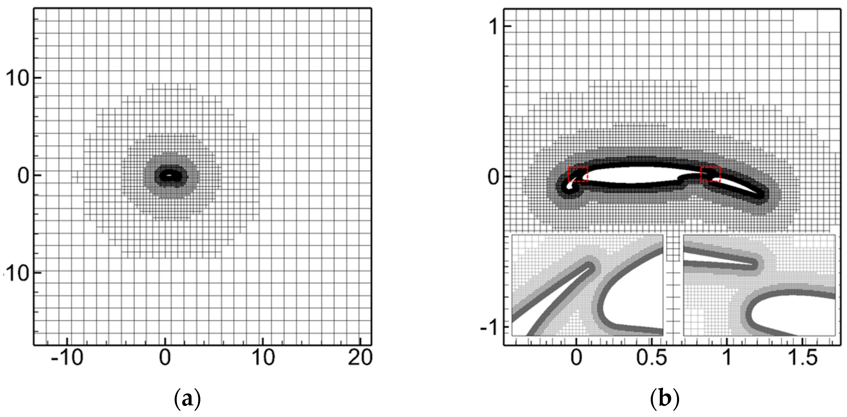
NHLP three−segment wing computational grids. (a) Global grids layout; (b) near-wall grids (the red box indicates the magnification of a local grid).
Figure 13.
NHLP three−segment wing computational grids. (a) Global grids layout; (b) near-wall grids (the red box indicates the magnification of a local grid).

Figure 14.
NHLP three−segment wing grid distribution before and after adaptation. (a) Initial grid; (b) after AMR.
Figure 14.
NHLP three−segment wing grid distribution before and after adaptation. (a) Initial grid; (b) after AMR.

Figure 15.
AMR process variation curves of grid quantity and residuals, and surface pressure coefficient curves. (a) Grid quantity and residuals; (b) surface pressure curves.
Figure 15.
AMR process variation curves of grid quantity and residuals, and surface pressure coefficient curves. (a) Grid quantity and residuals; (b) surface pressure curves.

Figure 16.
NHLP three-segment wing Ma flow field distribution before and after adaptation. (a) Initial grid; (b) after AMR.
Figure 16.
NHLP three-segment wing Ma flow field distribution before and after adaptation. (a) Initial grid; (b) after AMR.

Figure 17.
NHLP three-segment wing flow field distribution of turbulence viscosity coefficient before and after adaptation. (a) Initial grid; (b) after AMR.
Figure 17.
NHLP three-segment wing flow field distribution of turbulence viscosity coefficient before and after adaptation. (a) Initial grid; (b) after AMR.

Figure 18.
Sphere case computational domain and grid distribution diagram. (a) Global grid layout (the blue line represents the schematic of the computational domain size); (b) near-wall grid.
Figure 18.
Sphere case computational domain and grid distribution diagram. (a) Global grid layout (the blue line represents the schematic of the computational domain size); (b) near-wall grid.

Figure 19.
Flow field and grid distribution around the sphere in adaptive process. (a) Initial grid; (b) after two AMR processes; (c) after six AMR processes.
Figure 19.
Flow field and grid distribution around the sphere in adaptive process. (a) Initial grid; (b) after two AMR processes; (c) after six AMR processes.

Figure 20.
Pressure coefficient distribution diagram of sphere surface. (a) The front of the sphere; (b) the back of the sphere.
Figure 20.
Pressure coefficient distribution diagram of sphere surface. (a) The front of the sphere; (b) the back of the sphere.


Table 1.
Forward facing step case grid setup.
| Grid Type | Dimensionless Time | Number of Grids (×103) |
|---|---|---|
| Uni-level = 3 | 2.1 | 64.5 |
| Uni-level = 5 | 32.3 | 1032.2 |
| AMR-level = 3 | 1.0 | 31.6 |
| AMR-level = 5 | 6.3 | 163.7 |
Table 2.
Comparison of drag coefficients for supersonic sphere with experimental results.
| Grid Type | Number of Grids (×104) | Cd |
|---|---|---|
| Bailey and Hiatt [41] | / | 0.97 |
| Initial grid | 138 | 1.062 |
| After AMR | 417 | 0.988 |
Disclaimer/Publisher’s Note: The statements, opinions and data contained in all publications are solely those of the individual author(s) and contributor(s) and not of MDPI and/or the editor(s). MDPI and/or the editor(s) disclaim responsibility for any injury to people or property resulting from any ideas, methods, instructions or products referred to in the content. |
© 2024 by the authors. Licensee MDPI, Basel, Switzerland. This article is an open access article distributed under the terms and conditions of the Creative Commons Attribution (CC BY) license (https://creativecommons.org/licenses/by/4.0/).
Share and Cite
MDPI and ACS Style
Luo, C.; Zhou, D.; Meng, S.; Bi, L.; Wang, W.; Yuan, X.; Tang, Z. A Novel Cell-Based Adaptive Cartesian Grid Approach for Complex Flow Simulations. Appl. Sci. 2024, 14, 3692. https://doi.org/10.3390/app14093692
AMA Style
Luo C, Zhou D, Meng S, Bi L, Wang W, Yuan X, Tang Z. A Novel Cell-Based Adaptive Cartesian Grid Approach for Complex Flow Simulations. Applied Sciences. 2024; 14(9):3692. https://doi.org/10.3390/app14093692
Chicago/Turabian StyleLuo, Canyan, Dan Zhou, Shuang Meng, Lin Bi, Wenzheng Wang, Xianxu Yuan, and Zhigong Tang. 2024. "A Novel Cell-Based Adaptive Cartesian Grid Approach for Complex Flow Simulations" Applied Sciences 14, no. 9: 3692. https://doi.org/10.3390/app14093692
Note that from the first issue of 2016, this journal uses article numbers instead of page numbers. See further details here.