Construction Price Index Prediction through ARMA with Inflation Effect: Case of Thailand Construction Industry

Abstract

Over-budgeting due to inflation is a common phenomenon in the construction industry of both developed and developing countries. Inflation, with time changes, leaves an adverse effect on the project budget. Hence, this study aims to focus on the construction price index (CPI) behavior and inspect its correlation with inflation in Thailand’s construction industry as there has not been much work performed. The prediction of CPI was made from 2024 to 2028, relying on the data set from 2000 to 2023. The relationship between inflation and CPI categories helps in prediction by considering inflation as the independent variable and CPI (All Commodities, Lumber and Wood Products, Cement, and Iron Products) as the dependent variable that was incorporated in EViews to perform automated ARIMA forecasting. The correlation results show that out of four CPI, only Iron Products showed a significant relationship with inflation. For All Commodities, Lumber, and Wood Products, the predicted values were fluctuating, while for Cement and Iron Products, a clear seasonal pattern was observed. This prediction gives a direction to construction industry practitioners to make necessary adjustments to their budget estimation before signing the contract to overcome cost overrun obstruction.

1. Introduction

The construction industry provides multiple benefits beyond infrastructural development [1]. Not only does it boost the economy of a country, but it also creates a sustainable job market at every level [2,3]. The construction industry is also responsible for the integration of new technologies and guarding the environment [4,5]. Despite the numerous benefits of this sector, the construction industry still faces a multitude of challenges in project deliverables that reduce project productivity, efficiency, sustainability, and inclusive development [6,7,8]. One of the key problems is the overbudgeting of construction projects, which ultimately overburden the client’s finances [9]. This overbudgeting occurs when the estimated cost exceeds the final closure cost. Overall globally in construction projects, the budget deviation ranges between 5% and 10% [10,11]. Several factors contribute to the overbudgeting of a construction project and cause financial setbacks, e.g., wrong estimation [12], change order, vague project scope [13], inflation [14], and unforeseen conditions [15]. Moreover, project delays also escalate the construction goods and services cost, which burdens the budget [16,17]. The construction goods and services costs change with the time in which the role of inflation is not barred [18,19].

The impact of inflation is either direct or indirect on the construction industry [20,21]. Inflation not only has an impact on the Construction Price Index (CPI), but it also influences construction and other services [22]. The rise in inflation occurs when the cost of raw materials also increases in the market [23,24]. Materials are the fundamental elements for construction projects, and an increase in their prices directly influences the CPI. Inflation also elevates the labor wages to meet living expenses. Such inputs reflect an upward trend in CPI, which makes construction projects costly in general. The CPI is indirectly influenced by inflation as well due to adjustments in the interest rates [25,26]. The increase in inflation triggers the alarm in central banks, which then causes a rise in interest rates to maintain the economic threshold. Higher interest rates boost construction projects, deriving costs and ultimately overburdening financial costs [14]. This behavior adds an additional layer of cost to the project budget through CPI. As a result, more funds are needed to meet the basic demands of the construction projects. In a nutshell, the direct influence of inflation is through materials, labor, and machinery rates increases, and the indirect rate is through the interest rate [27,28].

With the help of the Scopus database [29], the keywords (“Inflation”, AND “Construction”, AND “Cost overrun”) were searched to feature the recent trend and linkage of the literature, which can be seen in Figure 1. It is obvious from the output that inflation in recent times is the thrust of the research, which is connected with budget control and construction projects and shows a relationship with cost overrun. In fact, inflation is the key indicator that impacts project costs by deviating them over time. Cost overrun through inflation is a global worry, and several studies have highlighted concerns about unsuccessful project completion due to overbudgeting. The literature underlines that this issue pertains to all the regions, either developing or developed, and the construction industry of all the countries is suffering [11,15,30,31,32,33,34,35,36,37,38,39,40,41,42,43,44,45,46,47,48,49]. Based on the carried-out literature, Figure 2 shows the world map highlighted with some of the regions marked with red in which the budget deviated from the original cost due to the inflation rate and ultimately led to project overbudgeting.

Jiang, Xu [50] emphasized construction prices’ reliable prediction as it impacts the decision-making of the contractors and the financiers. The long-run construction prices are dependent on the interest rate, population, and country’s income, while short-run construction prices are dependent on the price itself and the population. In this manner, the vector error correction (VEC) model was used to predict construction prices. The results indicate that, with the help of dummy variables, the forecasting is more efficient for the construction prices. The study showed promising results; however, instead of the dummy variables, the real-time data would be more promising. In another study, Shiha, Dorra [51] utilized a neural networks model to make the predictions of construction prices with the help of macroeconomic indicators. The model selection was based on mean absolute percentage error ranging from 4% to 11%. There were several limitations in the study, such as selection of the indicators and validation of the models, that leave a study gap for the future. Elfahham [52] draws a comparison between time series analysis, neural networks, and regression models to forecast construction cost indexes. Based on means absolute error and means squared error, it was observed that by using autoregressive time series, the outcome is better in comparison to the other two used methods for prediction.

Inflation in the economy portrays an expansion in prices, which is why it becomes essential to monitor the price shift [53]. So far, it is evident that inflation has ruined the mode of construction [53], and Thailand’s construction industry is also responding in the same manner as other countries’ construction industries [54]. In 2022, Thailand’s construction market value reached $23.7 billion, and a 3% growth is expected in the next four years [55]. The Thailand construction industry is facing several challenges; cost overrun is the major one, hindering the overall sustainable growth of the industry. The major influential factor that triggers this problem is inflation, which changes the prices of goods and services required for construction projects.

One main aspect that was not considered in previous studies is the inflation rate impact on the deviation of the construction price index. Musarat, Alaloul [56] explored this issue where the impact of the inflation rate was utilized to forecast the construction rates by using the time series analysis; however, the results were limited to the Malaysian industry and could further be extended to the other ASEAN regions to draw a comparison. Although the study methodology is aligned with the current work, this study focuses on the construction prices index rather than the construction rates that have not been addressed previously by adapting the time series analysis. Thus, this study stacks the focus on inflation mobility’s impact on the CPI over time. The CPI is important to estimate the cost and set up the budget before the bidding process. It is one of the key indicators of the cost level, leveling up the value for experts to understand the construction industry environment [57,58,59,60]. Hence, the CPI prediction is essential to boost the construction industry’s performance [52,61]. Currently, no such study is available for Thailand’s construction industry to incorporate the CPI in budgeting upon evaluating a relationship with inflation. Hence, the objective of this study is to evaluate the behavior of CPIs with time and assess the impact of inflation on shifting performance. Four CPIs were taken into consideration for further analysis, which are All Commodities, Lumber and Wood Products, Cement, and Iron Products. Moreover, time series analysis was opted to predict the future price indexes. The inflation issue requires vital attention in altering the construction price indexes that can be adapted initially at the time of contract allotment, which is the focus of this study. Besides inflation impact, there could be other possible reasons for the construction price deviation that led to project cost overrun, e.g., supply and demand, economic conditions, government policies, raw material prices, oil prices, and global market trends, etc.

Looking into the objectives, the following research questions were established:

• Do CPIs show any deviations in Thailand’s construction industry?
• Does inflation have any correlation with the CPIs in Thailand’s construction industry?
• Does Automated Autoregressive Integrated Moving Average (ARIMA) provide significant forecasting of CPIs?

The argument of this study is not based on low or high inflation in any country; rather it focuses on how the inflation rate deviates the prices in the construction market, which ultimately leads to cost overrun of a construction project. The scope of this study was limited to exploring the relationship between inflation and CPI in Thailand’s construction industry. The literature also supports auto machine learning [62]; however, this study utilized automated ARIMA forecasting, which has shown promising forecasting results for construction elements in the past [56]. Also, for the prediction of four CPIs, only the ARIMA model of time series analysis was considered without making any comparisons with other existing models due to the fact that the focus was kept on developing a strategy to make CPIs adjustments in the budget rather than drawing the comparison among the model for better predictions. Moreover, within the ARIMA model, there are several runs that give the best-suited value combination for the predictions. This study will help construction industry practitioners understand the seriousness of the matter and choose the outcome that will increase project productivity.

2. Research Method

The methodology of the study is divided into several steps. Initially, the mean and standard deviation of the construction index were evaluated, and then the percentage deviation was computed. Afterward, the linearity and nonlinearity of the data were determined as the correlation test selection was based on the data behavior. In the end, the prediction of the CPI was anticipated. For the mentioned processes, several tools such as Microsoft Excel (Version 2403, Build 17425.20176), Statistical Package for Social Sciences (SPSS-27), and EViews 12 SV were employed.

2.1. Inflation Rate and CPI Data Collection

The inflation rate and CPI data were collected from the web sources [63,64]. The data availability was from 2000–2023; the inflation rate was available annually while the CPI was monthwise. The CPI was comprised of four main categories: All Commodities, Lumber and Wood Products, Cement, and Iron Products. The inflation rate is reflected in Figure 3, while CPIs can be seen in Section 3.1.1. Over time, the inflation rate of Thailand has not been statistically significant and has fluctuated over time. The highest inflation appeared in 2022 and 2008 with rates of 6.08% and 5.47%, while the lowest was in 2020/2009 and 2015, with rates of −0.85% and −0.90%, respectively. The increase in inflation was due to high energy and food prices [4,65], while the decrease occurred due to a massive fall in global oil prices [3,66].

2.2. Descriptive Analysis

As the CPI data was monthwise, initially it was converted into yearly data by taking the average. This helps to calculate the arithmetic mean, standard deviation, and percentage deviation more appropriately [28,67]. The percentage deviation was computed using the following equation:

$$PercentageDeviation=\frac{(Currenttime-Previoustime)}{Previoustime}\times 100$$

(1)

2.3. Linear and Nonlinear Data Behavior

Before conducting further analysis, it is important to verify the data’s behavior as the correlation test selection is based on it. There are two ways to estimate whether the data is linear or nonlinear: (1) estimate the difference between two datasets where the outcome should be equal to 1, and (2) plot a graph among them [68]. In this study, both methods were adopted to indicate the data behavior.

Table 1. Nonlinearity of data.

Year Difference	Inflation Rate (Δx)	All Commodities (Δy)	Δy/Δx
2000–2001	0.00040	8.53	21,312.50
2001–2002	−0.00930	1.86	−199.82
2002–2003	0.01100	17.56	1596.21
2003–2004	0.00960	25.07	2611.11
2004–2005	0.01780	−0.06	−3.28
2005–2006	0.00100	10.12	10,116.67
2006–2007	−0.02400	13.78	−574.31
2007–2008	0.03230	50.60	1566.56
2008–2009	−0.06320	−45.10	713.61
2009–2010	0.04100	6.82	166.26
2010–2011	0.00560	19.29	3444.94
2011–2012	−0.00800	11.54	−1442.71
2012–2013	−0.00830	2.97	−358.43
2013–2014	−0.00280	2.41	−860.12
2014–2015	−0.02800	−17.53	626.19
2015–2016	0.01090	−8.80	−807.34
2016–2017	0.00480	−113.17	−23,576.39
2017–2018	0.00390	5.34	1369.66
2018–2019	−0.00350	−2.68	766.67
2019–2020	−0.01560	−3.65	233.97
2020–2021	0.02080	16.43	790.06
2021–2022	0.04850	2.69	55.50
2022–2023	−0.04730	−109.54	2315.89

shows the difference in output between the inflation rate and All Commodities. Here it can be seen that the difference is not equal to 1. Similarly, Figure 4 indicates the distance among the variables from the plotted imaginary linear line. Both methods classify the data behavior as nonlinear.

2.4. Correlation Coefficient

The correlation coefficient test varies as per the data behavior. For linear data, preferably the Pearson correlation is favorable, while for nonlinear data, Spearman correlation is recommended as it is a nonparametric measure [28,69,70]. As the data behavior portrays a nonlinear behavior, the Spearman correlation was embraced in this study.

The correlation coefficient value ranges from 0.00 to 1.00, where the positive value shows the relationship in the same direction while the negative value shows the relationship in the opposite direction. The range is further categorized into five subcategories: very weak, weak, moderate, strong, and very strong relationships. The values are kept as 0.00–0.19, 0.20–0.39, 0.40–0.59, 0.60–0.79, and 0.80–1.0, respectively.

2.5. Time Series Analysis

Time series analysis is the key method in research for understanding data performance and forecasting it. It has been utilized in several fields, and due to promising outcomes, it is still considered one of the most reliable forecasting methods to date [71,72,73]. One such astonishing forecasting method in time series is the Autoregressive Integrated Moving Average (ARIMA) as this model is a combination of three models that provides more accurate forecasting [19]. In this study, automated ARIMA forecasting was performed using EViews 12 SV. This software performs several runs on the data and provides the best model combination for forecasting. To have better-forecasted results, a higher number of observations is essential. In this case, the month-wise data was considered, where the data from January 2000 to December 2016 was reflected as a train while the data from January 2017 to December 2023 was reflected as a test. The prediction of CPI was functioned from 2024 to 2028.

3. Results and Discussion

This section demonstrates the descriptive analysis outcome of inflation and CPIs, where initially mean, standard deviation, and percentage deviation were computed. Then the Spearman correlation coefficient was calculated to find the relation between inflation and CPIs. In the end, automated ARIMA forecasting analysis was performed for construction price index forecasting. The description of all the analysis is provided below.

3.1. Construction Price Index Descriptive Outcome

3.1.1. Mean and Standard Deviation

Mean and standard deviation were computed for the four CPIs, as shown in Figure 5 and Figure 6. The highest mean was observed for Cement, with a 272.20 price index, and the lowest for All Commodities, with a 265.32 price index. In terms of standard deviation, the lowest value was for All Commodities at 60.74, indicating a lesser deviation in the price index, while the highest deviation was observed for Iron Products at 73.32, showing a much higher deviation in comparison to the other construction price index categories.

3.1.2. Percentage Deviation

The percentage deviation was computed for inflation and all the construction price indexes during each year. The results can be seen in Figure 7. In Figure 7a, the deviation of inflation can be seen where the highest positive deviation was recorded during 2021–2022 and 2009–2010 with a percentage of 4.85 and 4.10, while the highest negative deviation was reported during 2022–2023 and 2008–2009 with a percentage of −4.73 and −6.32, respectively. This indicates the instability of the Thailand inflation rate due to several factors that have a significant impact on inflation dynamics. The factors include retail energy, goods and services prices, and public policies [11]. In Figure 7b, the deviation of All Commodities can be seen where the highest positive deviation was recorded during 2007–2008 and 2003–2004 with a percentage of 17.14 and 10.17, while the highest negative deviation was reported during 2022–2023 and 2016–2017 with a percentage of −49.25 and −35.65, respectively. In Figure 7c, the deviation of Lumber and Wood Products can be seen where the highest positive deviation was recorded during 2018–2019 and 2008–2009 with a percentage of 10.69 and 12.25, while the highest negative deviation was reported during 2022–2023 and 2016–2017 with a percentage of −47.74 and −39.72, respectively. In Figure 7d, the deviation of Cement can be seen where the highest positive deviation was recorded during 2010–2011 and 2003–2004 with a percentage of 10.44 and 17.20, while the highest negative deviation was reported during 2022–2023 and 2016–2017 with a percentage of −51.83 and −39.96, respectively. In Figure 7e, the deviation of Iron Products can be seen where the highest positive deviation was recorded during 2020–2021 and 2007–2008 with a percentage of 33.88 and 38.38, while the highest negative deviation was reported during 2022–2023 and 2008–2009 with a percentage of −46.65 and −31.15, respectively.

Overall, the maximum positive deviation was scattered during the years 2000 to 2023, which is in line with the findings of the Musarat, Alaloul [28] study, where the prices of the materials show a positive deviation from 2013 to 2018. The negative deviation for the majority of the price indexes occurred during 2022–2023, which indicates the decrease in prices that could have arisen due to the decrease in inflation, which deviated up to −4.73%, showing a positive relationship. To strengthen the argument further, a correlation test was performed between inflation and CPIs; the details can be seen in the next section.

3.2. Spearman Correlation

As the data possess a nonlinear behavior, the Spearman test was performed to compute the influential relationship between inflation and CPIs. The outcome of the correlation coefficient can be seen in

Table 2. Spearman correlation coefficient.

Correlation	Inflation	All Commodities	Lumber and Wood Products	Cement	Iron Products
Inflation	1.000	0.380	0.110	0.232	0.547 **
All Commodities	0.380	1.000	0.800 **	0.917 **	0.900 **
Lumber and Wood Products	0.110	0.800 **	1.000	0.693 **	0.761 **
Cement	0.230	0.917 **	0.693 **	1.000	0.747 **
Iron Products	0.547 **	0.900 **	0.761 **	0.747 **	1.000

** Correlation is significant at the 0.01 level (two-tailed).

. At a 0.01 level, Iron Products showed a significant relationship with inflation. For other categories, it appeared weak and moderate, implying that the inflation rate directly influences the prices of iron products. In contrast, other categories are not that much affected by the push of inflation. The findings are in line with Musarat, Alaloul [27], where the inflation rate showed a moderate impact on the deviation of construction rates.

3.3. Construction Index Forecasting

From the Spearman correlation coefficient, it is obvious that inflation has a significant impact on Iron Products CPI; hence, in this manner, the forecasting of this category was estimated by considering inflation as the influential factor, mainly an independent variable. For the other CPI categories, such as All Commodities, Lumber and Wood Products, and Cement, the forecasting of construction indexes was made without considering the influence of inflation. The forecasting was pursued through EViews 12 SV, where the automated ARIMA forecasting method was applied. The prediction was made from the year 2024 to 2028, mainly five years in a row where the data for training purposes was considered from January 2000 to December 2016, while testing was pursued from January 2017 to December 2023. ARIMA is comprised of three major parts, i.e., AR (autoregressive), I (integrated), and MA (moving average). In automated ARIMA forecasting, the maximum value for AR was taken as 4, for I as 2, and for MA as 4 as well. Also, the maximum seasonality of AR and MA was considered as 2. The purpose of setting up the indicators at the maximum is that the automated ARIMA forecasting analysis runs several models, out of which the best model with a precise indicators combination gives accurate predictions over time.

3.3.1. Inflation Forecasting

The inflation data was available from 2000 to 2023 annually, and it was converted into monthly data to increase the number of observations and provide a better analysis. To incorporate the impact of inflation on construction indexes, initially, it was solely forecasted for the next 5 years. The sample was considered from 2000M01 to 2016M12, covering 204 observations, and the forecast length was 144. Out of 225 performed ARMA models, the best-suited model to predict the inflation rate was (2,0)(2,2). In contrast, Musarat, Alaloul [56] also predicted the inflation rate using the ARIMA model where (2,2)(0,0) was the best-estimated model. The model selection is based on the AIC value, which was 1.61. The lesser the AIC value, the better the model. Figure 8a shows the actual and predicted values of the inflation rate. It can be observed that the test data from 2016 to 2023 shows some fluctuations; however, over time, a gradual increase can be seen in inflation, implying its stability with the passage of time. Figure 8b shows the comparison of best-suited forecasting results with the other run models. The highlighted red line shows the smoothness in the predicted value.

Table 3. Equation output of inflation forecast.

Variable	Coefficient	Std. Error	t-Statistic	Prob.
C	2.194712	0.606260	3.620085	0.0004
AR(1)	0.985125	0.670448	1.469353	0.1433
AR(2)	−0.007173	0.693668	−0.010341	0.9918
SAR(12)	0.186447	0.316973	0.588211	0.5571
SAR(24)	0.307683	0.032796	9.381837	0.0000
MA(12)	−0.972736	11288.41	−8.62 × 10−5	0.9999
MA(24)	−0.027260	656.6765	−4.15 × 10−5	1.0000
SIGMASQ	0.246019	206.1922	0.001193	0.9990
R-squared	0.920968	Mean dependent var		2.232941
Adjusted R-squared	0.918146	S.D. dependent var		1.768686
S.E. of regression	0.506024	Akaike info criterion		1.633577
Sum squared resid	50.18785	Schwarz criterion		1.763700
Log-likelihood	−158.6249	Hannan–Quinn criterion		1.686214
F-statistic	326.2883	Durbin–Watson stat		1.990976
Prob(F-statistic)	0.000000

shows the equation output of the (2,0)(2,2) model, and for each variable, the coefficient, standard error, t-statistic, and prob. can be seen. The R-squared value was 0.920968, while the adjusted R-squared value was 0.918146. The Schwarz criterion, which is the goodness of fit of a statistical model, was 1.763700.

3.3.2. All Commodities Forecasting

The availability of All Commodities data was from 2000 to 2023 monthwise, which gives sufficient observations for better analysis. The sample was considered from 2000M01 to 2016M12, covering 203 observations, and the forecast length was 144. Out of 225 performed ARMA models, the best-suited model to predict the All Commodities price index was (4,3)(0,0). The model selection is based on the AIC value, which was −6.03. Here, the impact of inflation was not considered due to the fact that it does not show an acceptable relationship with this construction index as per the output came from the Spearman correlation. Figure 9a shows the actual and predicted values of All Commodities. It can be observed that the test data from 2016 to 2023 shows some fluctuations in a downward direction; however, over time, a gradual increase can be seen in CPI, implying an increase in the rate of passage of time. Figure 9b shows the comparison of best-suited forecasting results with the other run models. The highlighted red line shows the smoothness in the predicted value.

Table 4. Equation output of All Commodities forecast.

Variable	Coefficient	Std. Error	t-Statistic	Prob.
C	0.002159	0.000940	2.295630	0.0228
AR(1)	0.177184	0.068835	2.574051	0.0108
AR(2)	0.709834	0.090861	7.812312	0.0000
AR(3)	0.483491	0.091907	5.260653	0.0000
AR(4)	−0.462280	0.083747	−5.519974	0.0000
MA(1)	0.483692	56.75715	0.008522	0.9932
MA(2)	−0.528842	100.5943	−0.005257	0.9958
MA(3)	−0.954838	291.9963	−0.003270	0.9974
SIGMASQ	0.000127	0.000808	0.156629	0.8757
R-squared	0.408387	Mean dependent var		0.001879
Adjusted R-squared	0.383991	S.D. dependent var		0.014662
S.E. of regression	0.011508	Akaike info criterion		−6.030707
Sum squared resid	0.025691	Schwarz criterion		−5.883816
Log-likelihood	621.1168	Hannan–Quinn criterion		−5.971281
F-statistic	16.73963	Durbin–Watson stat		1.964301
Prob(F-statistic)	0.000000

shows the equation output of the (4,3)(0,0) model, and for each variable, the coefficient, standard error, t-statistic, and prob. can be seen. The R-squared value was 0.408387, while the adjusted R-squared value was 0.383991. The Schwarz criterion, which is the goodness of fit of a statistical model, was −5.883816. The Schwarz criterion is a tool that is required for better model selection on the same set of data.

3.3.3. Lumber and Wood Products Forecasting

The availability of Lumber and Wood Products data was from 2000 to 2023 monthwise, which gives sufficient observations for better analysis. The sample was considered from 2000M01 to 2016M12, covering 204 observations, and the forecast length was 144. Out of 225 performed ARMA models, the best-suited model to predict the Lumber and Wood Products price index was (2,0)(2,0). The model selection is based on the AIC value, which was −5.45. Here, the impact of inflation was not considered due to the fact that it does not show an acceptable relationship with this construction index. Figure 10a shows the actual and predicted values of Lumber and Wood Products. It can be observed that the test data from 2016 to 2023 shows the same pattern over time, implying that the predicted indexes will act in the same manner as in the past. Figure 10b shows the comparison of best-suited forecasting results with the other run models. The highlighted red line shows that the model provided the seasonal pattern in the predicted value. This indicates that Lumber and Wood Products have seasonality in the indexes.

Table 5. Equation output of Lumber and Wood Products forecast.

Variable	Coefficient	Std. Error	t-Statistic	Prob.
C	5.557116	0.074450	74.64229	0.0000
AR(1)	0.111829	0.112344	0.995417	0.3207
AR(2)	0.164115	0.065529	2.504461	0.0131
SAR(12)	−0.000860	0.001455	−0.590980	0.5552
SAR(24)	0.998264	0.000936	1066.249	0.0000
SIGMASQ	0.000120	3.42 × 10−6	35.20780	0.0000
R-squared	0.997961	Mean dependent var		5.557793
Adjusted R-squared	0.997909	S.D. dependent var		0.243412
S.E. of regression	0.011131	Akaike info criterion		−5.446017
Sum squared resid	0.024530	Schwarz criterion		−5.348425
Log-likelihood	561.4937	Hannan–Quinn criterion		−5.406539
F-statistic	19377.10	Durbin–Watson stat		2.047059
Prob(F-statistic)	0.000000

shows the equation output of the (2,0)(2,0) model, and for each variable, the coefficient, standard error, t-statistic, and prob. can be seen. The R-squared value was 0.997961, while the adjusted R-squared value was 0.997909. The Schwarz criterion, which is the goodness of fit of a statistical model, was −5.348425.

3.3.4. Cement Forecasting

The availability of Cement data was from 2000 to 2023 monthwise, which gives sufficient observations for better analysis. The sample was considered from 2000M01 to 2016M12, covering 203 observations, and the forecast length was 144. Out of 225 performed ARMA models, the best-suited model to predict the Cement price index was (2,2)(2,2). The model selection is based on the AIC value, which was −3.36. The findings are in contrast with the Musarat, Alaloul [56] study, where the best-suited model appeared as (1,0)(0,0). It is worth mentioning that the impact of inflation was taken into account in the highlighted study. Here, in the present study, the impact of inflation was not considered due to the fact that it does not show an acceptable relationship with this construction index. Figure 11a shows the actual and predicted values of Cement. It can be observed that the test data from 2016 to 2023 shows the same pattern over time, implying that the predicted indexes will act in the same manner as in the past. Figure 11b shows the comparison of best-suited forecasting results with the other run models. The highlighted red line shows that the model provided the seasonal pattern in the predicted value. This indicates that Cement has seasonality in the indexes.

Table 6. Equation output of Cement forecast.

Variable	Coefficient	Std. Error	t-Statistic	Prob.
C	5.569992	0.088445	62.97714	0.0000
AR(1)	1.396289	0.101657	13.73529	0.0000
AR(2)	−0.910738	0.103743	−8.778795	0.0000
SAR(12)	−0.005831	0.017116	−0.340685	0.7337
SAR(24)	0.980879	0.012204	80.37355	0.0000
MA(1)	−1.427389	14.39211	−0.099179	0.9211
MA(2)	0.999984	20.14361	0.049643	0.9605
SMA(12)	−0.035521	0.201697	−0.176112	0.8604
SMA(24)	0.515332	0.054369	9.478397	0.0000
SIGMASQ	0.001107	0.010875	0.101761	0.9191
R-squared	0.984891	Mean dependent var		5.58293
Adjusted R-squared	0.984186	S.D. dependent var		0.271303
S.E. of regression	0.034117	Akaike info criterion		−3.355757
Sum squared resid	0.224647	Schwarz criterion		−3.192545
Log-likelihood	350.6093	Hannan–Quinn criterion		−3.289728
F-statistic	1397.853	Durbin–Watson stat		1.87343
Prob(F-statistic)	0.000000

shows the equation output of the (2,2)(2,2) model, and for each variable, the coefficient, standard error, t-statistic, and prob. can be seen. The R-squared value was 0.984891, while the adjusted R-squared value was 0.984186. The Schwarz criterion, which is the goodness of fit of a statistical model, was −3.192545.

3.3.5. Iron Products Forecasting

The availability of Iron Products data was from 2000 to 2023 monthwise, which gives sufficient observations for better analysis. The sample was considered from 2000M01 to 2016M12, covering 204 observations, and the forecast length was 144. Out of 225 performed ARMA models, the best-suited model to predict the Iron Products price indexes was (3,3)(2,2). The output is in contrast with the Sen, Roy [74] findings, where the best-suited ARIMA model was (1,0,0)(0,1,1) for Indian pig iron. The model selection is based on the AIC value which was 7.79. Here, in the current study, the impact of inflation was considered due to the fact that, it showed an acceptable relationship with this construction index. Figure 12a shows the actual and predicted values of Iron Products. It can be observed that the test data from 2016 to 2023 shows the same pattern over time, implying that the predicted indexes will act in the same manner as in the past. Figure 12b shows the comparison of best-suited forecasting results with the other run models. The highlighted red line shows that the model provided the seasonal pattern in the predicted value. This indicates that Iron Products have seasonality in the indexes.

Table 7. Equation output of Iron Products forecast.

Variable	Coefficient	Std. Error	t-Statistic	Prob.
INFLATION	0.275909	0.497121	0.555013	0.5796
AR(1)	−0.823	0.167117	−4.924672	0.0000
AR(2)	0.967595	0.086061	11.24316	0.0000
AR(3)	0.803576	0.153786	5.225287	0.0000
SAR(12)	−0.33226	0.072482	−4.584061	0.0000
SAR(24)	0.651887	0.071521	9.11465	0.0000
MA(1)	0.933316	0.155323	6.008883	0.0000
MA(2)	−0.90411	0.137158	−6.59177	0.0000
MA(3)	−0.86965	0.126955	−6.850007	0.0000
SMA(12)	0.072988	0.072749	1.003285	0.3171
SMA(24)	0.828168	0.062154	13.32448	0.0000
SIGMASQ	70.21861	5.094261	13.78387	0.0000
R-squared	0.988449	Mean dependent var		272.4676
Adjusted R-squared	0.986973	S.D. dependent var		78.15826
S.E. of regression	8.920823	Akaike info criterion		7.790796
Sum squared resid	14324.6	Schwarz criterion		8.181163
Log-likelihood	−770.6612	Hannan–Quinn criterion		7.948707
Durbin-Watson stat	1.967388

shows the equation output of the (3,3)(2,2) model, and for each variable, the coefficient, standard error, t-statistic, and prob. can be seen. The R-squared value was 0.988449, while the adjusted R-squared value was 0.986973. The Schwarz criterion, which is the goodness of fit of a statistical model, was 8.181163.

3.4. Discussion on Predicted CPIs

The predicted CPIs, along with inflation, can be seen in Figure 13. It is noticeable that more or less inflation will be stable and have a percentage near 2. For the CPI, all commodities will increase as time passes, hence increasing the prices of goods and services. This might be due to the supply and demand in Thailand’s construction industry in the near future. For Lumber and Wood Products, Cement, and Iron Products, the predicted construction indexes show fluctuation in rates, indicating that they will not follow a specific pattern and can vary over time depending on the construction and economic environment. Based on the AIC values, the predicted CPIs are in line with the findings of the Musarat, Alaloul [56] study, where the emphasis was on the impact of the inflation rate in deviating the construction project cost. Jiang, Xu [50] emphasize the prediction of CPI as the price indicators impact the decision-making of the contractors. Elfahham [52] argued that the pricing process is challenging, and a controlled CPI would help to balance the project cost. The focus of the current study was more on the importance of adjusting the inflation rate in budget estimates rather than drawing the model’s comparison. This study will help to incorporate the predicted CPIs more efficiently when required by the construction industry authorities to look into the project budget before its finalization. The forecasted results set a benchmark for how effectively the CPIs can be predicated before setting up the project budget.

4. Conclusions

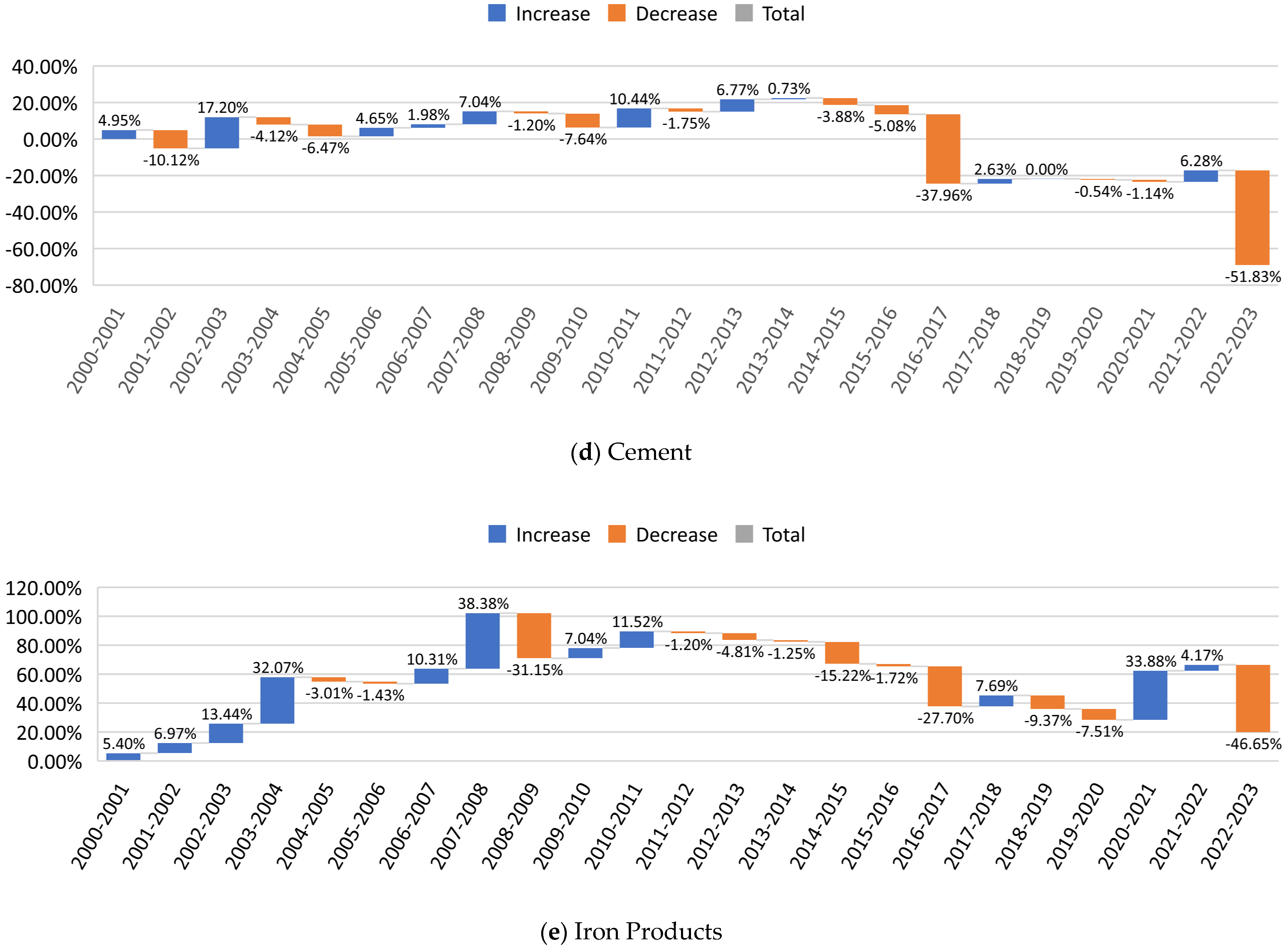
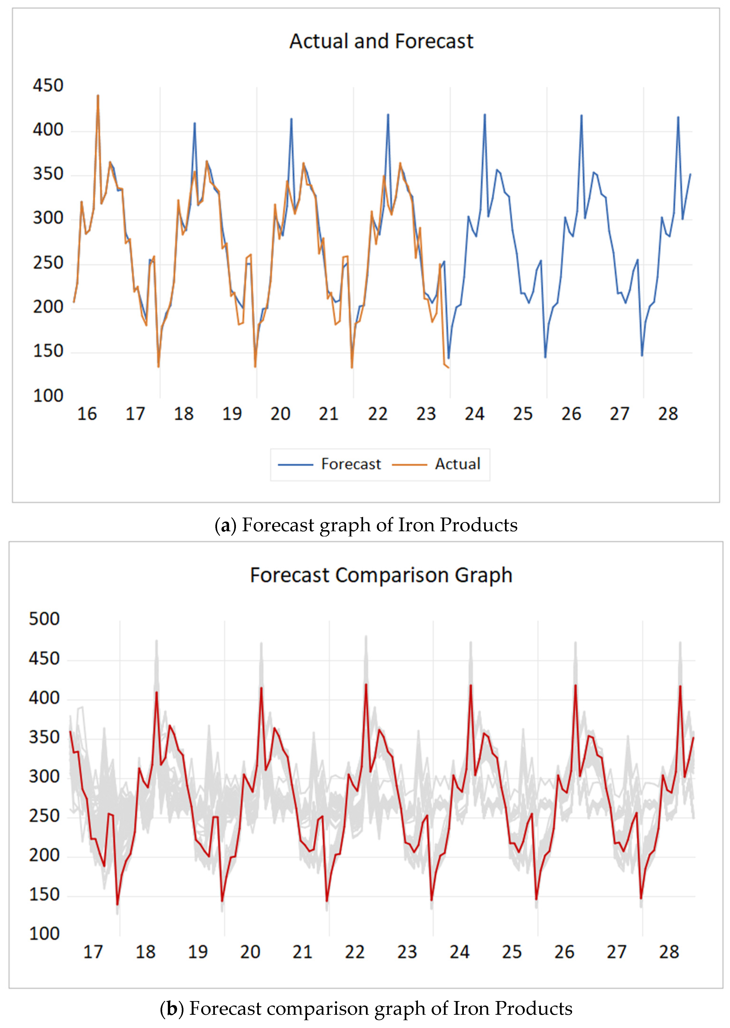
The construction price index (CPI) is the key indicator of the cost estimate as it helps to set up the project budget wisely. However, over time, the CPI becomes elevated, and the fluctuating behavior is unfavorable for all construction practitioners. Hence, this study focuses on evaluating the changing behavior of CPIs with the inflation effect and the prediction of CPIs to overcome the project overbudgeting problem. Four CPIs, i.e., All Commodities, Lumber and Wood Products, Cement and Iron Products, were deemed dependent, whereas inflation was independent. Initially, descriptive analysis, percentage deviation, and correlation coefficient were computed. The deviation showed that the data behavior was nonconsistent and the indexes changed over time, while the correlation coefficient showed a significant relationship between inflation and Iron Products price indexes. After evaluating the correlation, ARIMA forecasting was performed to predict construction price indexes. Inflation as an independent variable was considered for Iron Products price indexes only, whereas a seasonal pattern showed up for Cement and Iron Products. In contrast, for All Commodities and Lumber and Wood Products, the data did not show any specific pattern. This study gives a predicted value for all the CPIs that can be considered for budget adjustments before the time of contract allotment, which will help construction practitioners reduce the cost overrun impact due to price deviation. The forecasted values show the pattern in the coming years that can be considered at the initial budgeting time to avoid over-budgeting.

5. Implications and Limitations

This study provides the prediction of CPI based on the impact of inflation on the construction industry of Thailand. As a theoretical implication, this study clarifies the need for CPI prediction with inflation adjustment. As a practical implication, the formulated strategy can help construction industry practitioners make necessary adjustments. This prediction will help in making modifications at contract time to avoid the cost overrun effects. The predictions will also help to present the best-suited project budget at the time of bidding. This will reduce the impact of cost deviation from the initial budget to the final budget and will reduce the burden on the financiers. Although, as a case study, the data from the Thailand construction industry was analyzed, it can be implicated in other regions’ construction industries as well by keeping the impact of influential factors such as the inflation rate. Further, the results are useful for other ASEAN countries as well, as they have similarities in construction industry characteristics due to their close geographical proximity, interconnected economies, and comparable stages of development.

Some limitations occurred while pursuing this study. The data was taken from 2000 to 2023, and for a better understanding of its behavior, the observations could be increased. Only four categories were taken into account for construction price indexes. Other individual categories need vital attention to study the data behavior more precisely. Automated ARIMA forecasting was implemented on the gathered data. However, other techniques such as ANN, CNN, or AI tools could also be utilized to predict the construction price indexes. Lastly, in this study, inflation was considered as the independent variable; however, other factors may also be measured in the future in order to evaluate the influential relationship with construction price indexes.

References

1. Ullah, K.; Lill, I.; Witt, E. An overview of BIM adoption in the construction industry: Benefits and barriers. In Proceedings of the 10-th Nordic Conference on Construction Economics and Organization (CEDO), Tallinn, Estonia, 7–8 May 2019; Emerald Publishing Limited: Bingley, UK, 2019. [Google Scholar] [CrossRef]
2. Benachio, G.L.F.; Freitas, M.D.C.D.; Tavares, S.F. Circular economy in the construction industry: A systematic literature review. J. Clean. Prod. 2020, 260, 121046. [Google Scholar] [CrossRef]
3. Alaloul, W.S.; Musarat, M.A.; Rabbani, M.B.A.; Iqbal, Q.; Maqsoom, A.; Farooq, W. Construction sector contribution to economic stability: Malaysian GDP distribution. Sustainability 2021, 13, 5012. [Google Scholar] [CrossRef]
4. Bello, S.A.; Oyedele, L.O.; Akinade, O.O.; Bilal, M.; Delgado, J.M.D.; Akanbi, L.A.; Ajayi, A.O.; Owolabi, H.A. Cloud computing in construction industry: Use cases, benefits and challenges. Autom. Constr. 2020, 122, 103441. [Google Scholar] [CrossRef]
5. Datta, S.D.; Tayeh, B.A.; Hakeem, I.Y.; Abu Aisheh, Y.I. Benefits and Barriers of Implementing Building Information Modeling Techniques for Sustainable Practices in the Construction Industry—A Comprehensive Review. Sustainability 2023, 15, 12466. [Google Scholar] [CrossRef]
6. Abioye, S.O.; Oyedele, L.O.; Akanbi, L.; Ajayi, A.; Delgado, J.M.D.; Bilal, M.; Akinade, O.O.; Ahmed, A. Artificial intelligence in the construction industry: A review of present status, opportunities and future challenges. J. Build. Eng. 2021, 44, 103299. [Google Scholar] [CrossRef]
7. Azis, A.A.A.; Memon, A.H.; Rahman, I.A.; Nagapan, S.; Latif, Q.B.A.I. Challenges faced by construction industry in accomplishing sustainablity goals. In Proceedings of the 2012 IEEE Symposium on Business, Engineering and Industrial Applications, Bandung, Indonesia, 23–26 September 2012; IEEE: Piscataway, NJ, USA, 2012. [Google Scholar]
8. Hossain, M.U.; Ng, S.T.; Antwi-Afari, P.; Amor, B. Circular economy and the construction industry: Existing trends, challenges and prospective framework for sustainable construction. Renew. Sustain. Energy Rev. 2020, 130, 109948. [Google Scholar] [CrossRef]
9. Nileshbhai, M.M.; Solanki, J.V. Reducing over budgeting in construction project. Int. Res. J. Eng. Technol. 2020, 7, 6906–6911. [Google Scholar]
10. Memon, A.H.; Rahman, I.A. Budget overrun issues in construction projects of southern part of Malaysia. Int. J. Civ. Eng. Built. Environ. 2014, 1, 1–6. [Google Scholar]
11. Haslinda, A.N.; Xian, T.W.; Norfarahayu, K.; Hanafi, R.M.; Fikri, H.M. Investigation on the factors influencing construction time and cost overrun for high-rise building projects In penang. J. Phys. Conf. Ser. 2018, 995, 012043. [Google Scholar] [CrossRef]
12. El-Kholy, A. Predicting cost overrun in construction projects. Int. J. Constr. Eng. Manag. 2015, 4, 95–105. [Google Scholar]
13. Herrera, R.F.; Sánchez, O.; Castañeda, K.; Porras, H. Cost overrun causative factors in road infrastructure projects: A frequency and importance analysis. Appl. Sci. 2020, 10, 5506. [Google Scholar] [CrossRef]
14. Abdul Nabi, M.; El-adaway, I.H.; Assaad, R.H. Modeling Inflation Transmission among Different Construction Materials. J. Constr. Eng. Manag. 2024, 150, 04024024. [Google Scholar] [CrossRef]
15. Albtoush, A.F.; Doh, S. A Review on causes of cost overrun in the construction projects. Int. J. N. Innov. Eng. Technol. 2019, 12, 15–22. [Google Scholar]
16. Larsen, J.K.; Shen, G.Q.; Lindhard, S.M.; Brunoe, T.D. Factors affecting schedule delay, cost overrun, and quality level in public construction projects. J. Manag. Eng. 2016, 32, 04015032. [Google Scholar] [CrossRef]
17. Evikbaş, M.; Işık, Z. An overarching review on delay analyses in construction projects. Buildings 2021, 11, 109. [Google Scholar] [CrossRef]
18. Babalola, A.J.; Aderogba, A.M.; Adetunji, O.O. Inflation and Cost Overrun in Public Sector Construction Projects in Nigeria. ECS Trans. 2022, 107, 16137–16147. [Google Scholar] [CrossRef]
19. Boulic, M.; Phipps, R.; Wang, Y.; Vignes, M.; Adegoke, N.A. Validation of low-cost air quality monitoring platforms using model-based control charts. J. Build. Eng. 2024, 82, 108357. [Google Scholar] [CrossRef]
20. Dabara, D.; Chiwuzie, A.; Omotehinshe, O.; Soladoye, J.O. Impact of inflation on indirect real estate investments in Nigeria. In Proceedings of the European Real Estate Society (ERES) Conference, Cergy-Pontoise, France, 3 July 2019. [Google Scholar]
21. Akal, A.Y. Inflation and Reinforced Concrete Materials: An Investigation of Economic and Environmental Effects. Sustainability 2023, 15, 7687. [Google Scholar] [CrossRef]
22. Pandey, R.K.; Khan, A.; Scholar, P. Impact of inflation rate on construction project: A review. Int. J. Sci. Res. Civ. Eng. 2023, 7, 23–29. [Google Scholar]
23. Mohamed, E.; Mahmoud, S. An assessment of the impact of inflation on the prices of selected construction materials in Sudan. Int. J. Multidiscip. Res. Publica. 2020, 2, 41–44. [Google Scholar]
24. Bansal, K.K.; Ahalawat, N. Effect of inflation on supply chain model with exponential demand. Multi. Discip. Edu. Glob. Quest 2013, 2, 33–50. [Google Scholar]
25. Yu, K.-W. The Economics of Construction Price Inflation in the UK: Measurement, Output and Productivity; UCL (University College London): London, UK, 2014. [Google Scholar]
26. Shapton, B.J. Development of Unit Price Indices and Estimating Inflation for Potable Water and Wastewater Pipeline Capital Works Construction; University of Waterloo: Waterloo, ON, Canada, 2017. [Google Scholar]
27. Musarat, M.A.; Alaloul, W.S.; Liew, M.S.; Maqsoom, A.; Qureshi, A.H. The effect of inflation rate on CO2 emission: A framework for malaysian construction industry. Sustainability 2021, 13, 1562. [Google Scholar] [CrossRef]
28. Ali Musarat, M.; Salah Alaloul, W.; Liew, M.; Maqsoom, A.; Hannan Qureshi, A. Investigating the impact of inflation on building materials prices in construction industry. J. Build. Eng. 2020, 32, 101485. [Google Scholar] [CrossRef]
29. Scopus. Available online: https://www.scopus.com/results/results.uri?sort=plf-f&src=s&st1=%22Construction%22+AND+%22Cost+overrun%22&sid=eab5489189080ccde14e6b0fcfa8376a&sot=b&sdt=b&sl=48&s=TITLE-ABS-KEY%28%22Inflation%22+AND+%22Construction%22+AND+%22Cost+overrun%22%29&origin=searchbasic&editSaveSearch=&yearFrom=Before+1960&yearTo=Present&sessionSearchId=eab5489189080ccde14e6b0fcfa8376a&limit=10 (accessed on 27 December 2023).
30. Barrera, M.A.; Sabbatella, I.; Serrani, E. Macroeconomic barriers to energy transition in peripheral countries: The case of Argentina. Energy Policy 2022, 168, 113117. [Google Scholar] [CrossRef]
31. Shah, R.K. An exploration of causes for delay and cost overruns in construction projects: Case study of Australia, Malaysia & Ghana. J. Adv. Coll. Eng. Manag. 2016, 2, 41–55. [Google Scholar] [CrossRef]
32. Kumar, H.; Skelton, L.; Kularatne, I. Causes of cost overrun in construction projects in Auckland. N. Z. J. Appl. Bus. Res. 2021, 17, 19–33. [Google Scholar]
33. Pyataev, M. Cost overruns in Russian transport megaprojects. In International Scientific Siberian Transport Forum; Springer: Berlin/Heidelberg, Germany, 2021. [Google Scholar]
34. Saeidlou, S.; Ghadiminia, N. A construction cost estimation framework using DNN and validation unit. Build. Res. Inf. 2024, 52, 38–48. [Google Scholar] [CrossRef]
35. Samarghandi, H.; Mousavi, S.; Taabayan, P.; Mir Hashemi, A.; Willoughby, K. Studying the reasons for delay and cost overrun in construction projects: The case of Iran. J. Constr. Dev. Ctries. 2016, 21, 51–84. [Google Scholar] [CrossRef]
36. Niazi, G.A.; Painting, N. Significant factors causing cost overruns in the construction industry in Afghanistan. Procedia Eng. 2017, 182, 510–517. [Google Scholar] [CrossRef]
37. Oghenekevwe, O.; Olusola, O.; Chukwudi, U.S. An assessment of the impact of inflation on construction material prices in Nigeria. PM World J. 2014, 3, 1–22. [Google Scholar]
38. Goyal, S. Effect of inflation on project costs in Rajasthan. In Proceedings of the SARC-CAN International Conference, New Delhi, India, 12 March 2017. [Google Scholar]
39. Tang, C.F. The effect of real wages and inflation on labour productivity in Malaysia. Int. Rev. Appl. Econ. 2014, 28, 311–322. [Google Scholar] [CrossRef]
40. Leavitt, D.; Ennis, S.; McGovern, P. The Cost Escalation of Rail Projects: Using Previous Experience to Re-Evaluate the Calspeed Estimates; University of California at Berkely: Berkeley, CA, USA, 1993. [Google Scholar]
41. Enshassi, A.; Al-Najjar, J.; Kumaraswamy, M. Delays and cost overruns in the construction projects in the Gaza Strip. J. Financ. Manag. Prop. Constr. 2009, 14, 126–151. [Google Scholar] [CrossRef]
42. Olawale, Y.A.; Sun, M. Cost and time control of construction projects: Inhibiting factors and mitigating measures in practice. Constr. Manag. Econ. 2010, 28, 509–526. [Google Scholar] [CrossRef]
43. Aziz, R.F. Factors causing cost variation for constructing wastewater projects in Egypt. Alex. Eng. J. 2013, 52, 51–66. [Google Scholar] [CrossRef]
44. Amusan, L.M.; Afolabi, A.; Ojelabi, R.; Omuh, I.; Okagbue, H.I. Data exploration on factors that influences construction cost and time performance on construction project sites. Data Brief 2018, 17, 1320–1325. [Google Scholar] [CrossRef] [PubMed]
45. Johnson, R.M.; Babu, R.I.I. Time and cost overruns in the UAE construction industry: A critical analysis. Int. J. Constr. Manag. 2018, 20, 402–411. [Google Scholar] [CrossRef]
46. Le-Hoai, L.; Lee, Y.D.; Lee, J.Y. Delay and cost overruns in Vietnam large construction projects: A comparison with other selected countries. KSCE J. Civ. Eng. 2008, 12, 367–377. [Google Scholar] [CrossRef]
47. Kaliba, C.; Muya, M.; Mumba, K. Cost escalation and schedule delays in road construction projects in Zambia. Int. J. Proj. Manag. 2009, 27, 522–531. [Google Scholar] [CrossRef]
48. Alinaitwe, H.; Apolot, R.; Tindiwensi, D. Investigation into the causes of delays and cost overruns in Uganda’s public sector construction projects. J. Constr. Dev. Ctries. 2013, 18, 33. [Google Scholar]
49. Aslam, B.; Maqsoom, A.; Inam, H.; Basharat, M.U.; Ullah, F. Forecasting Construction Cost Index through Artificial Intelligence. Societies 2023, 13, 219. [Google Scholar] [CrossRef]
50. Jiang, H.; Xu, Y.; Liu, C. Construction price prediction using vector error correction models. J. Constr. Eng. Manag. 2013, 139, 04013022. [Google Scholar] [CrossRef]
51. Shiha, A.; Dorra, E.M.; Nassar, K. Neural networks model for prediction of construction material prices in Egypt using macroeconomic indicators. J. Constr. Eng. Manag. 2020, 146, 04020010. [Google Scholar] [CrossRef]
52. Elfahham, Y. Estimation and prediction of construction cost index using neural networks, time series, and regression. Alex. Eng. J. 2019, 58, 499–506. [Google Scholar] [CrossRef]
53. Tembo, M.; Mwanaumo, E.M.U.; Kahanji, C. An Investigation into Construction Tender-Price Inflation: A Documentary Review. J. Constr. Bus. Manag. 2023, 6, 17–32. [Google Scholar]
54. Makulsawatudom, A.; Emsley, M.; Sinthawanarong, K. Critical factors influencing construction productivity in Thailand. J. KMITNB 2004, 14, 1–6. [Google Scholar]
55. Thailand Construction Market Size, Trend Analysis by Sector, Competitive Landscape and Forecast to 2027. Available online: https://www.globaldata.com/store/report/thailand-construction-market-analysis/ (accessed on 31 December 2023).
56. Musarat, M.A.; Alaloul, W.S.; Liew, M. Incorporating inflation rate in construction projects cost: Forecasting model. Heliyon 2024, 10, e26037. [Google Scholar] [CrossRef] [PubMed]
57. Joukar, A.; Nahmens, I. Volatility forecast of construction cost index using general autoregressive conditional heteroskedastic method. J. Constr. Eng. Manag. 2016, 142, 04015051. [Google Scholar] [CrossRef]
58. Faghih, S.A.M.; Kashani, H. Forecasting construction material prices using vector error correction model. J. Constr. Eng. Manag. 2018, 144, 04018075. [Google Scholar] [CrossRef]
59. Lei, T.; Li, R.Y.M.; Jotikastira, N.; Fu, H.; Wang, C. Prediction for the Inventory Management Chaotic Complexity System Based on the Deep Neural Network Algorithm. Complexity 2023, 2023, 9369888. [Google Scholar] [CrossRef]
60. Li, R.Y.M.; Fong, S.; Chong, K.W.S. Forecasting the REITs and stock indices: Group method of data handling neural network approach. Pac. Rim Prop. Res. J. 2016, 23, 123–160. [Google Scholar] [CrossRef]
61. Hwang, S. Time series models for forecasting construction costs using time series indexes. J. Constr. Eng. Manag. 2011, 137, 656–662. [Google Scholar] [CrossRef]
62. Li, R.Y.M.; Song, L.; Li, B.; Crabbe, M.J.C.; Yue, X.-G. Predicting Carpark Prices Indices in Hong Kong Using AutoML. Comput. Model. Eng. Sci. 2022, 134, 2247–2282. [Google Scholar] [CrossRef]
63. Thailand Inflation Rate 1960–2023. Available online: https://www.macrotrends.net/countries/THA/thailand/inflation-rate-cpi#:~:text=Thailand%20inflation%20rate%20for%202022,a%200.36%25%20decline%20from%202018 (accessed on 10 December 2023).
64. Summary Table on Construction Materials Price Index 2000–2023. Available online: http://www.indexpr.moc.go.th/price_present/csi/stat/other/indexcsi1_eng.asp?list_year=2566 (accessed on 10 December 2023).
65. Thailand’s Inflation Rate in 2022 Was Close to Its Projection and Expected to Decelerate in 2023. Available online: https://uploads.tpso.go.th/3.1_press_eng_dec_2022.pdf (accessed on 25 December 2023).
66. Inflation Dynamics and Inflation Expectations in Thailand. Available online: https://www.bis.org/publ/bppdf/bispap89y.pdf (accessed on 25 December 2023).
67. Musarat, M.A.; Alaloul, W.S.; Liew, M. Inflation rate and labours’ wages in construction projects: Economic relation investigation. Eng. Constr. Arch. Manag. 2021, 29, 2461–2494. [Google Scholar] [CrossRef]
68. Alaloul, W.S.; Musarat, M.A.; Liew, M.; Qureshi, A.H.; Maqsoom, A. Investigating the impact of inflation on labour wages in Construction Industry of Malaysia. Ain Shams Eng. J. 2021, 12, 1575–1582. [Google Scholar] [CrossRef]
69. Luo, L.; Meng, L.; Yan, Z.; Millcock, S.; Li, R.Y.M.; Chow, C. Enhancing Accessibility, Functionality and Meditation Design in a Suburban Activity Centre: A Case Study at Mawson Lakes Campus. J. Health Manag. 2023, 1–15, 09720634231205656. [Google Scholar] [CrossRef]
70. Myers, L.; Sirois, M.J. Spearman correlation coefficients, differences between. Encycl. Stat. Sci. 2004, 1, 12. [Google Scholar] [CrossRef]
71. Lim, B.; Zohren, S. Time-series forecasting with deep learning: A survey. Philos. Trans. R. Soc. A Math. Phys. Eng. Sci. 2021, 379, 20200209. [Google Scholar] [CrossRef] [PubMed]
72. De Gooijer, J.G.; Hyndman, R.J. 25 years of time series forecasting. Int. J. Forecast. 2006, 22, 443–473. [Google Scholar] [CrossRef]
73. Rabbani, M.B.A.; Musarat, M.A.; Alaloul, W.S.; Maqsoom, A.; Ayub, S.; Bukhari, H.; Altaf, M. A comparison between seasonal autoregressive integrated moving average (SARIMA) and exponential smoothing (ES) based on time series model for forecasting road accidents. Arab. J. Sci. Eng. 2021, 46, 11113–11138. [Google Scholar] [CrossRef]
74. Sen, P.; Roy, M.; Pal, P. Application of ARIMA for forecasting energy consumption and GHG emission: A case study of an Indian pig iron manufacturing organization. Energy 2016, 116, 1031–1038. [Google Scholar] [CrossRef]
Figure 1. Overlay visualization from keywords.
Buildings 14 01243 g001
Figure 2. World map showing countries with cost overrun issues due to inflation.
Buildings 14 01243 g002
Figure 3. Thailand inflation rate.
Buildings 14 01243 g003
Figure 4. Scattergram of inflation rate with price index.
Buildings 14 01243 g004
Figure 5. Construction categories prices index.
Buildings 14 01243 g005
Figure 6. Standard deviation of construction categories.
Buildings 14 01243 g006
Figure 7. Percentage deviation.
Buildings 14 01243 g007aBuildings 14 01243 g007b
Figure 8. Inflation forecasting analysis.
Buildings 14 01243 g008
Figure 9. All Commodities forecasting analysis.
Buildings 14 01243 g009
Figure 10. Lumber and Wood Products forecasting analysis.
Buildings 14 01243 g010
Figure 11. Cement forecasting analysis.
Buildings 14 01243 g011
Figure 12. Iron Products forecasting analysis.
Buildings 14 01243 g012
Figure 13. Predicted construction price indexes (January 2024 to December 2028).
Buildings 14 01243 g013