
Urban Building Height Extraction from Gaofen-7 Stereo Satellite Images Enhanced by Contour Matching


1
School of Remote Sensing Information Engineering, Wuhan University, Wuhan 430079, China
2
State Key Laboratory of Information Engineering in Surveying Mapping and Remote Sensing, Wuhan University, Wuhan 430079, China
3
School of Computer Science and Technology, Wuhan University of Science and Technology, Wuhan 430065, China
*
Author to whom correspondence should be addressed.
Remote Sens. 2024, 16(9), 1556; https://doi.org/10.3390/rs16091556
Submission received: 15 March 2024
/
Revised: 21 April 2024
/
Accepted: 24 April 2024
/
Published: 27 April 2024
(This article belongs to the Special Issue 3D Reconstruction and Mobile Mapping in Urban Environments Using Remote Sensing)
Abstract
:The traditional method for extracting the heights of urban buildings involves utilizing dense matching algorithms on stereo images to generate a digital surface model (DSM). However, for urban buildings, the disparity discontinuity issue that troubles the dense matching algorithm makes the elevations of high-rise buildings and the surrounding areas inaccurate. The occlusion caused by trees in greenbelts makes it difficult to accurately extract the ground elevation around the building. To tackle these problems, a method for building height extraction from Gaofen-7 (GF-7) stereo images enhanced by contour matching is presented. Firstly, a contour matching algorithm was proposed to extract accurate building roof elevation from GF-7 images. Secondly, a ground filtering algorithm was employed on the DSM to generate a digital elevation model (DEM), and ground elevation can be extracted from this DEM. The difference between the rooftop elevation and the ground elevation represents the building height. The presented method was verified in Yingde, Guangzhou, Guangdong Province, and Xi’an, Shaanxi Province. The experimental results demonstrate that our proposed method outperforms existing methods in building height extraction concerning accuracy.
1. Introduction
A recent study on urban growth typology shows that there has been a large increase in high-rise buildings in China [1]. The building height information holds significant application value in various fields, such as urban local climate [2,3], building energy consumption evaluation [4,5], urban pollution dispersion [6,7], urban carbon emissions evaluation [8,9], earthquake perception [10], and urban 3D reconstruction [11]. Therefore, building height extraction over large regions is essential for a comprehensive understanding of an urban development.
Remote sensing technology is the most commonly used method for building height extraction. Typically, building heights are extracted through three approaches: airborne light detection and ranging (LiDAR), side-looking radar imagery, and high-resolution optical imagery. Airborne LiDAR allows high accuracy measurements [12]. These algorithms extract buildings and their heights through point cloud classification algorithms [13,14] or utilize building footprints from digital maps to reconstruct buildings in three dimensions [15]. However, airborne LiDAR has limitations in coverage and high costs. Algorithms utilizing side-looking radar imagery often require building footprints obtained from digital maps or other sources [16,17,18,19]. Nevertheless, with the side-looking geometry, radar images usually record signals from a mixture of different microwave scattering mechanisms, leading to relatively high uncertainties of building height extraction [20].
In contrast, optical satellite imagery has high acquisition efficiency and offers abundant spatial details, hence being widely applied in building height extraction. For single optical satellite images, the shadow-based method is commonly employed to extract building heights. This method utilizes the relationship between the sun, satellite, building rooftops, and shadows in the imagery to extract building height [21,22,23,24,25]. However, the shadow-based method faces difficulties in building height extraction when buildings are short or when shadows are occluded by other objects [26].
For stereo images, a common method involves generating a DSM through dense matching and projecting building footprints or rooftops onto the DSM to extract building heights. Liu et al. [27] utilized semi-global matching (SGM) [28] to generate a DSM, employed morphological filtering [29] on the DSM to generate DEM, and finally derived the normalized DSM (nDSM) using the maximum values within the nDSM as the building heights. Wang et al. [30] improved DEM generation with the more precise cloth simulation filter (CSF) method [31]. To address the issue of missing rooftop elevations in a DSM generated by the SGM algorithm, Zhang et al. [26] proposed a contour-constrained rooftop matching algorithm for building height extraction.
With the rapid development of deep learning, deep learning methods have been widely applied in dense matching [32,33,34], opening up new possibilities for building height extraction. For instance, Chen et al. [35] utilized a DSM generated by deep learning algorithms in building height extraction. End-to-end deep learning methods have also been proposed for building height extraction in stereo images. Cao et al. [36] designed the network to extract buildings and their heights from multi-view, multi-spectral images. This method does not rely on dense matching algorithms but requires known building height data for training.
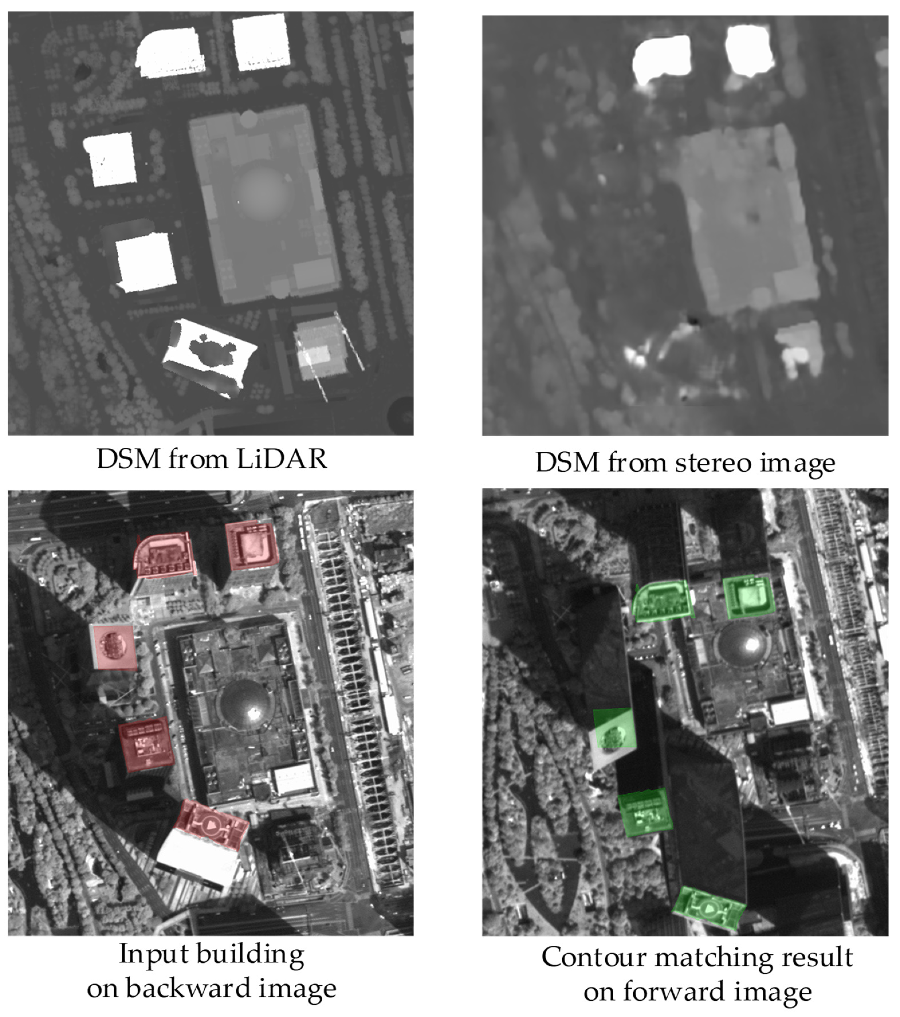
The GF-7 satellite is capable of capturing panchromatic stereo images spanning 20 km in width with a resolution finer than 0.8 m. Its backward camera holds a tilt angle of −5 degrees, while the forward camera tilts at 26 degrees, maintaining a favorable balance between minimized occlusion and a wider stereo intersection angle. It offers valuable data for building height extraction. However, limitations in resolution and the forward camera tilt angle challenge the application of current dense matching algorithms, hindering their accuracy in building height extraction. Relevant research indicates that many 3D breaklines are modeled as more or less smooth transitions from ground level to building level [37]. Figure 1a,b illustrates the impact of this problem on building height extraction. This DSM is generated by the algorithm of He et al. [32] using GF-7 stereo images of Xi’an. In Figure 1a, inaccuracies in the ground elevation around the building are evident. While the actual ground elevation is 355 m, the DSM shows elevations higher than the reality. Figure 1b shows inaccuracies in high-rise buildings. The actual building height is 350 m, with a rooftop elevation of 702 m. There are substantial differences in shape and elevation between the reconstructed buildings and their actual counterparts. Figure 1c illustrates occlusion caused by trees in Guangzhou. Detailed data for both Xi’an and Guangzhou are provided in Section 3.1. These challenges lead to difficulties for algorithms relying on a DSM in accurately extracting the building heights.
To improve the building height estimation accuracy, we proposed a contour matching enhanced building height extraction method. Instead of overlaying the building contours on the DSM directly, we used a contour matching algorithm to obtain more accurate rooftop elevation and ground filtering to generate a DEM from the DSM for more robust ground elevation. Firstly, the given building contours, which can be in ground space or on a GF-7 backward image, are matched to GF-7 forward images with a contour matching, and the rooftop elevation can be extracted using the geometric relationship between the matched building rooftop. Secondly, the ground elevation around the building can be extracted from the DEM, which filters the DSM generated from GF-7 stereo images. GF-7 multispectral images are utilized to improve the accuracy of ground filtering. Finally, the difference between the rooftop elevation and the ground elevation represents the building height.
The main contributions of this paper are as follows:
- An object-level contour matching algorithm is proposed to extract the rooftop plane elevation. Contrary to the pixel-level dense matching, which can generate smooth transitions in the DSM, the proposed algorithm, taking the rooftop as an object, can overcome the complex detail interruption of the rooftop.
- A ground filtering considering ground types is proposed for ground elevation extraction. Most existing ground filtering algorithms, which are designed for LiDAR cloud points with multi-echo, will not generate good DEM when applied directly to a satellite-DSM-generated DSM. In our new algorithm, we use multi-spectral imagery to assist in identifying non-ground points and inaccurate ground points in ground filtering algorithms.
Our paper is organized as follows: Section 2 of the paper extensively describes the extraction of the building height and discusses scenarios where multiple elevations exist for building rooftops. Section 3 of the paper demonstrates the effectiveness of this approach through experiments. The proposed algorithm is discussed in Section 4. Finally, Section 5 concludes this paper.
2. Methodology
The algorithm workflow for building height extraction is illustrated in Figure 2. The known data required in this algorithm include the GF-7 images, DSM generated from GF-7 stereo images, building footprints in the geographic coordinate system, or building rooftop contours in GF-7 backward images. The contour matching algorithm for building footprints (CM-F) is described in Algorithm 1. The building rooftop contours in GF-7 backward images may have unclear edges or may encompass podium buildings and building sides. Our algorithm utilizes the backward images to reduce the impact of unclear edges. Furthermore, it is possible to use differences between the forward and backward images to identify building sides and podium buildings. The contour matching algorithm for building rooftop contours (CM-R) is described in Algorithm 2.
| Algorithm 1. The contour matching algorithm for building footprint (CM-F) |
|
| Algorithm 2. The contour matching algorithm for building rooftop contour (CM-R) |
|
2.1. Image Contour Extraction
Building contour consists of a collection of edges formed by continuous curves or lines, which match with the edges extracted from the image in contour match. The Canny edge detection algorithm [38] is utilized to extract edges in the image as contour points. The gradient direction of the image is calculated as the contour point direction, as shown in Equation (1):
where and represent the gradients in the horizontal and vertical directions, respectively. In the arctan function, the signs of and are used to ensure that the gradient direction ranges from [−π, π].
This study extends the range of contour point direction values from the [0, π] as in conventional methods [39] to [−π, π]. Due to the parapet walls at the rooftop, there are two adjacent indistinguishable edges in the image. By expanding the range of gradient direction, these two edges can be distinguished based on their positive or negative gradient directions. An example is provided in Figure 3.
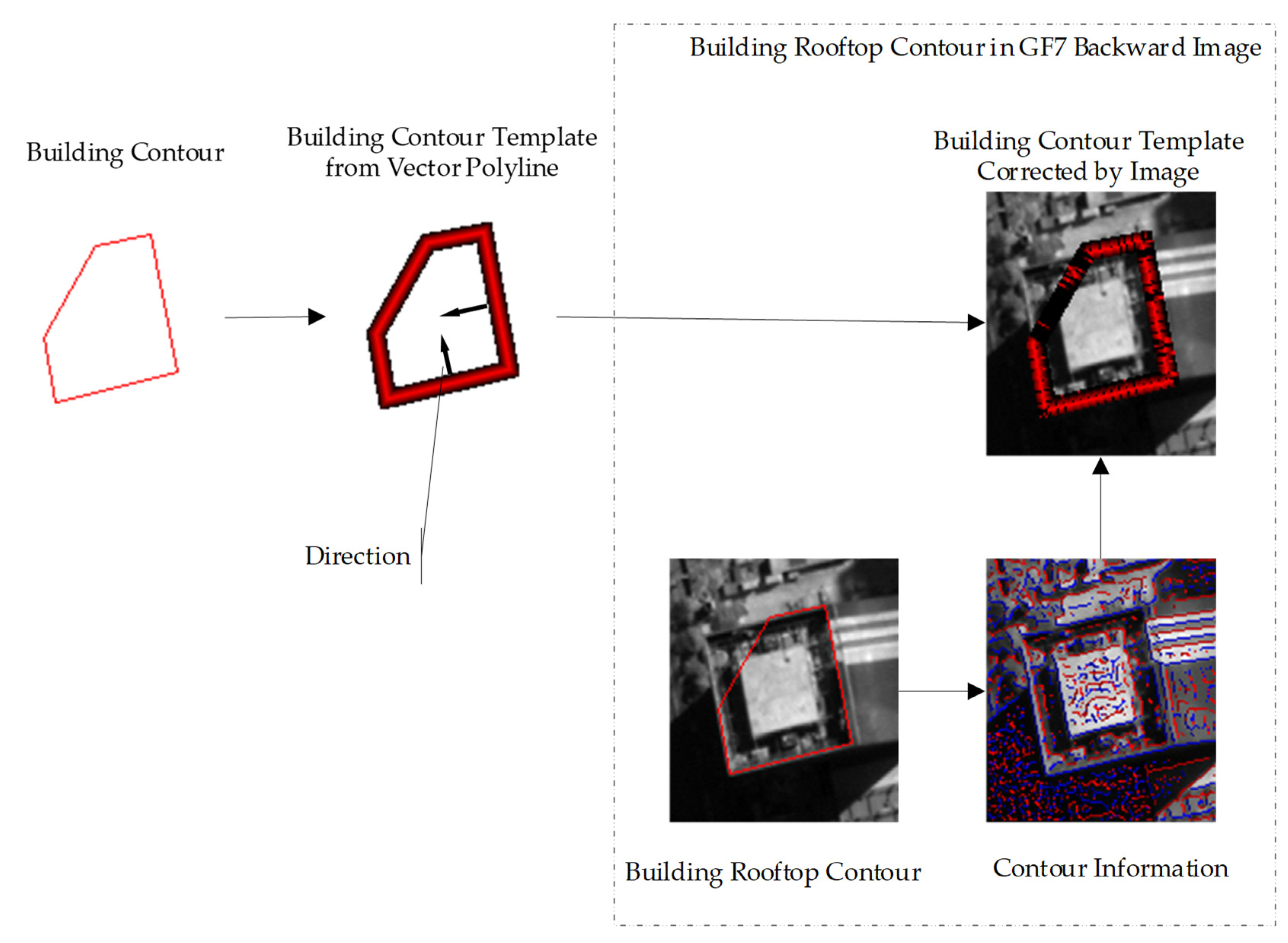
2.2. Building Contour Template Construction
Building contour templates are constructed to describe building rooftops. Figure 4 illustrates the process of building contour template construction. The vector polygon of the building is simplified by the Douglas algorithm [40]. Then, we created buffer zones for the edges of the vector polygon. The pixels within the buffer zone are considered potential contour points that constitute building contour templates. Their weights are calculated by the distance to the building edges, as shown in Equation (2).
Here, represents the buffer distance; denotes the distance from the point to the edge in pixels, where is negative when the point is inside the building contour.
The potential contour point direction is perpendicular to the corresponding edges of the polygon. As buildings in remote sensing images are generally brighter than other features [41], we set the potential contour point direction points inside the polygon. For any point on the edge, draw a perpendicular line to the edge. The potential contour points that the perpendicular line passes through are grouped as a set, denoted by . In contour matching, the matched contour of is found within the range of .
2.3. Contour Matching Degree Calculation and Building Contour Template Correction
The contour matching degree represents the similarity between the building rooftop and the contours within the image. The contour matching degree is calculated as follows: The building contour template is moved to the location of the candidate building rooftop in the image, and each potential contour point can correspond to an image pixel. When a corresponding image pixel is a contour point extracted from the image, the angle between the potential contour point direction and contour point direction is calculated, denoted as . Then, the weight of the contour point in the image is calculated using Equation (3).
In this equation, represents a penalty coefficient. In our study, is assigned a value of 0.5 experientially.
In set , the contour point with the maximum weight is matched with the , denoted as . We denote this maximum weight as , and the contour matching degree can be calculated using Equation (4). When the candidate building rooftop is changed, the building rooftop contour in the image will move along the epipolar line. Therefore, the building edges perpendicular to the epipolar line play an important role in roof elevation extraction. Consequently, by increasing the weights of contour points in these edges, more accurate rooftop elevations can be obtained, and the weighted contour matching degree is computed using Equation (5).
In this context, represents the total number of sets , and denotes the circumference of the building contour in pixels. The value of the weight function is determined by the edge where is located. When the angle between the edge and the epipolar line exceeds 60 degrees, = 2; otherwise, = 1.
In practical application, the input building rooftop contours extracted by the building extraction algorithm may have unclear edges. Building contour template correction can improve the accuracy of the algorithm in this case. By computing the contour matching degree between the building rooftop contour and the GF-7 backward image, the matched contour points in the backward image are found and used to recalculate the weights of the potential contour point. The corrected weights of the potential contour point are calculated as follows: for any set , if , then the distance between potential contour points within and is calculated. Subsequently, is used in Equation (2) to recalculate . If , the values of potential contour points in are set to 0. The correction results are illustrated in Figure 4.
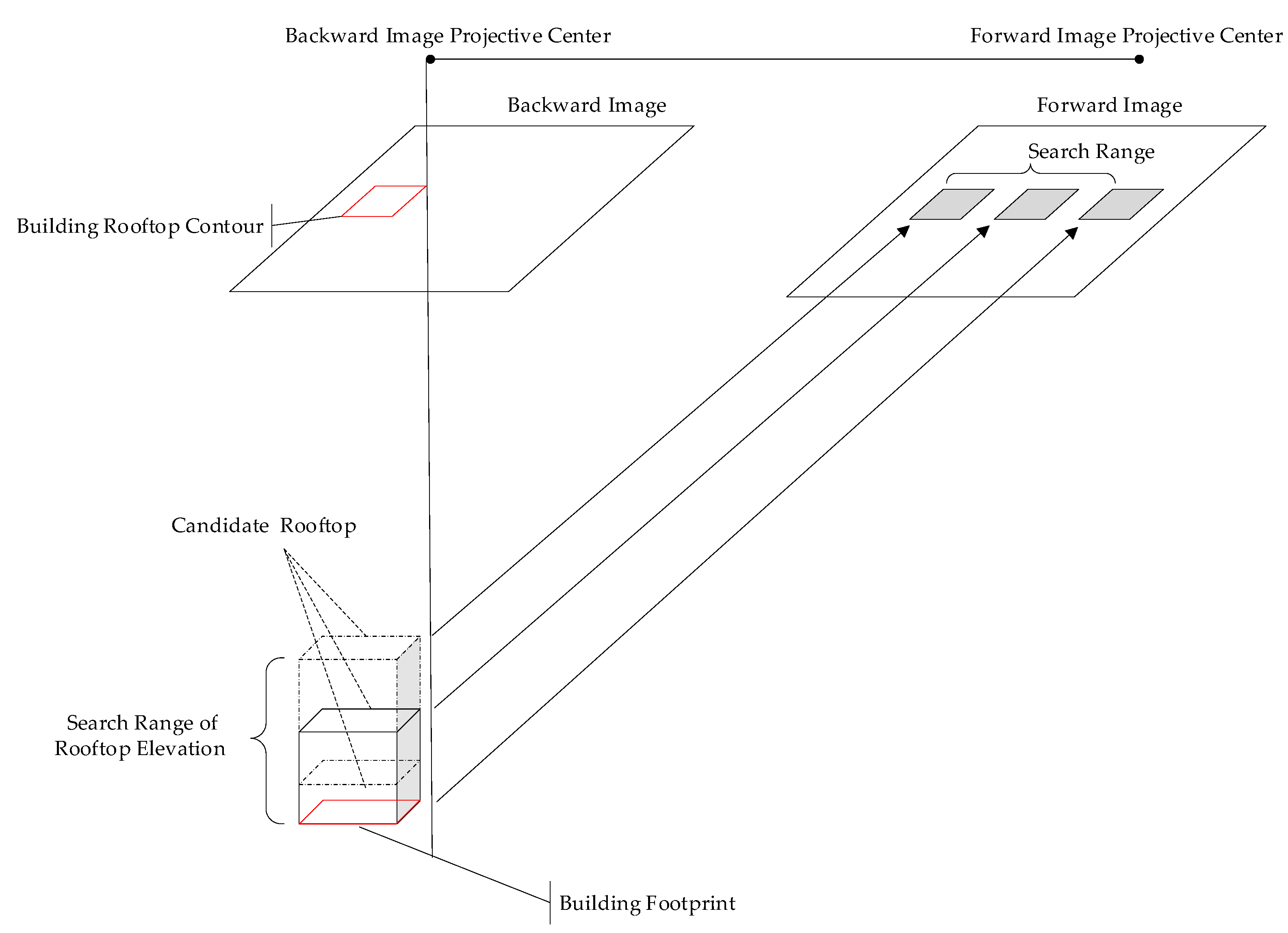
2.4. Building Rooftop Elevation Extraction
The principle of building rooftop elevation extraction is illustrated in Figure 5. According to known building contour, multiple candidate building rooftops can be obtained within the elevation search range of rooftop. These candidate rooftops are projected onto the GF-7 forward image using the rational function model and verified by contour matching.
The conventional contour matching method [39] sets a threshold for the contour matching degree and obtains the matched building contour based on the maximum value of the contour matching degree. In rooftop elevation extraction, multiple local maximum values of contour matching degree are caused by similar buildings or unclear building edges. The local maximum values lead to mismatches and significant errors. Therefore, our study utilizes elevation information from the DSM to filter out the local maximum values with significant errors.
The curve of contour matching degree versus candidate rooftop elevation is acquired at first. The elevation search range of the rooftop can be estimated using Equation (6).
where is set to be slightly greater than the estimated maximum building height, and is the minimum elevation within the building buffer zone.
For building footprints in geographic coordinates, the variation between adjacent candidate rooftop elevations is set based on image resolution and stereo intersection angle. For each within the range , the candidate building rooftop is projected onto the GF-7 forward image, and can be calculated using the method mentioned earlier. For the building rooftop contours in the backward image, the elevation search range of rooftop is transformed to the disparity search range of rooftop, designated as . For each integer within the range , the and rooftop elevation is calculated, allowing us to acquire the curve of versus rooftop elevation.
The minimum elevation and maximum elevation within the building buffer zone in the DSM are utilized to filter the local maximum value of contour matching degree. The local maximum values of contour matching degree are sorted in descending order, denoted as , and their corresponding rooftop elevations are denoted as . If condition is satisfied, it means the contour matching degree has a significant maximum value, and is the rooftop elevation. In the absence of a significant maximum value, two situations need to be distinguished. If any local maximum value satisfies , and the rooftop elevation satisfies , then is considered as the rooftop elevation. If condition is satisfied, it is considered that the corresponding building rooftop does not exist in the GF-7 forward image. This indicates that the building is occluded in the forward image or that the known building differs from reality.
2.5. Ground Elevation Extraction around the Building
Our proposed method utilizes the results of GF-7 multispectral image classification to enhance the accuracy of the DEM generated by the ground filtering algorithm. GF-7 multispectral images are employed to compute the normalized difference vegetation index (NDVI) and the normalized difference water index (NDWI), allowing for the classification of vegetation and water from the image. By projecting input buildings into the DSM, the building can be classified from the DSM. The non-ground points such as vegetation and buildings are removed from the DSM. Additionally, large water bodies lacking texture that tend to cause mismatches are also removed from the DSM.
Subsequently, inaccurate ground points around buildings and trees are removed. In Figure 6a, profile comparisons of DSMs from LiDAR and stereo images are presented for a building in Guangzhou. The red lines represent the DSM from stereo images, and the black represents the DSM from LiDAR. In the ground pointed by the arrow, the DSM from the stereo image is higher than the DSM from LiDAR. These points should be removed from the ground filter. Figure 6b illustrates the method for identifying inaccurate ground points. For each window near the building, we calculated the elevation change along four lines. If , the points on this line are considered as inaccurate points. Figure 6c shows a partial multispectral image of Guangzhou, Figure 6d shows the removed points in this image. This process ensures that the elevation of the occluded ground is estimated from nearby ground.
2.6. Segmentation of Building Rooftop Contours Containing Multiple Elevations
The material of the podium building and building side is similar to that of the main building rooftop, making it difficult to distinguish them in remote sensing images. Consequently, some building rooftop contours in input data encompass the podium building and building side. To address this problem, differences in building contour between forward and backward images are utilized to segment these building rooftop contours. The algorithm process is as follows:
| Algorithm 3. Building rooftop contour segmentation process |
|
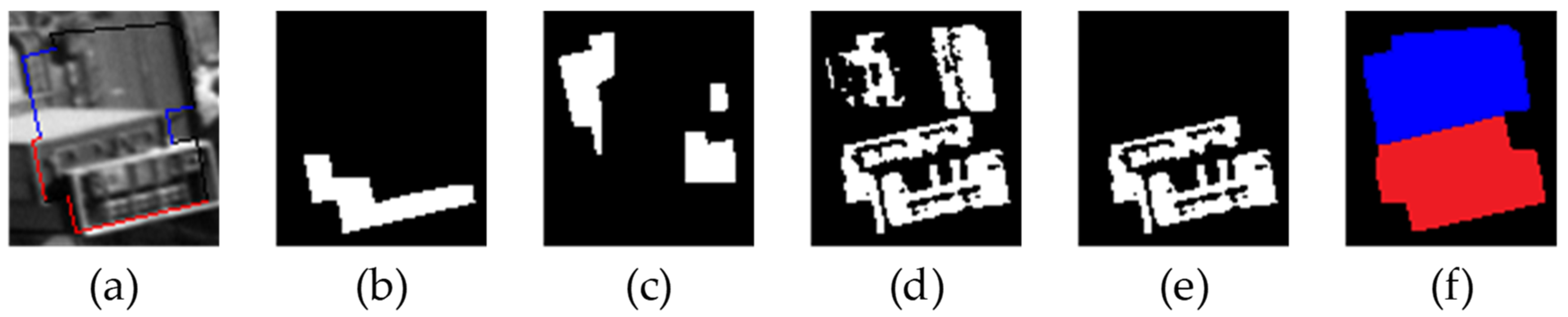
In contour matching, a matched building edge has a long enough parallel line in the image. We proposed a method to identify matched edges. We divide the building contour template into multiple subsets based on the edges in the building rooftop contours. For each subset, the total number of is denoted as . For each within the subset, the distance between and is calculated. To distinguish points inside the building contour from points outside the building contour, the distance of the point inside the building contour is set to a negative value. Considering that the lines in the image have dimensions, the distance intervals [,], [,], …, [,] are used to represent the parallel lines. The represents the width of the parallel line and is set to 2 pixels. If the distance between and belongs to any internal, belongs to this parallel line. The parallel line with the most contour points is the longest, denoting this contour point number as . When , the edge is considered as a matched edge. Set to represent matched edges set in the backward image, and to represent matched edges set in the forward image. Figure 7 shows two building rooftop contours and the corresponding , .
As shown in Figure 7, the matched edges are different in the forward and backward images. Due to the tilt angles, the building sides in the backward image are occluded in the forward images. Additionally, the relative location between the podium building and the main building has changed. The differences between and provide samples for building contour segmentation. Define the set of edges , where the edges in belong to the main building rooftop. Define the set of edges , where the edges in belong to the podium building rooftop. By buffering and intersecting it with the building contours, the samples of the main building are obtained. Similarly, applying these operations to provides samples of the podium building. In Figure 8a, the red edges represent , and the blue edges represent . Meanwhile, Figure 8b shows samples of the main building rooftop, and Figure 8c shows samples of the podium building.
The pixels within the building rooftop in the forward images are classified into main building pixels and podium building pixels based on their grayscale. The K-means clustering algorithm is employed to group these pixels into eight clusters. For each cluster, the numbers of pixels in main building samples and podium building samples are counted, separately. If the number of pixels in the main building samples exceeds those within the podium building samples, this cluster is considered as a part of the main building rooftop. The resulting main building rooftop from this process is depicted in Figure 8d. Due to the limitations of panchromatic images, pixels with the same grayscale as the main building rooftop are misclassified. To address this issue, the parts overlapping with the samples of the main building are preserved, illustrated in Figure 8e. Thereafter, the longest edge in the original building contour is found to assist in gap filling. For each pixel outside the main building rooftop, parallel and perpendicular lines of the longest edge are drawn. If both ends of the parallel or perpendicular lines intersect with the main building rooftop, the pixel is considered part of the main building rooftop. We denote the main building rooftop as , while the remaining building rooftop is a podium building, denoted as . Figure 8f shows the classification result, where the red area represents , and the blue area represents .
For podium building rooftop , the contour matching algorithm is executed. is identified as a podium building when a building rooftop is matched in the forward image. Otherwise, it is considered as occluded building sides. Following Zhang’s algorithm [26] as a reference, this paper conducted building contour segmentation experiments in Xi’an. Figure 9 shows the partial results of the building contour segmentation.
3. Results
3.1. Data Description and Experimental Area
This paper selected three regions—Yingde and Guangzhou in Guangdong Province, and Xi’an in Shaanxi Province—as experimental areas for the algorithm. Their basic details are as follows:
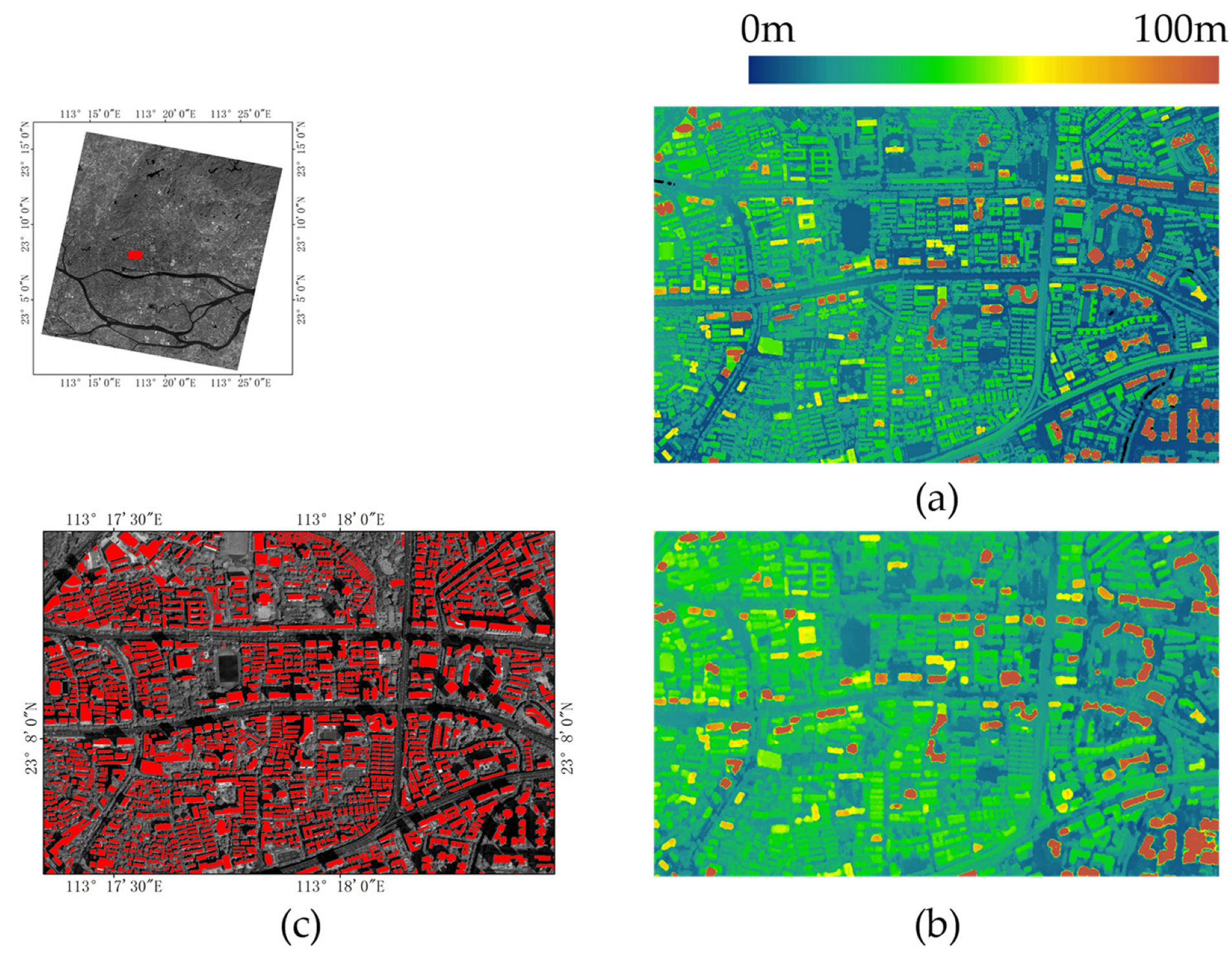
As for the Yingde experimental area, the GF-7 image was captured on 11 October 2020. The center coordinates of the backward image were 113.409°E and 24.326°N, with solar zenith and azimuth angles of 33.466° and 158.717°, respectively. A total of 841 building footprints within this experimental area were acquired. The images and the building footprints of the Yingde experimental area are shown in Figure 10. The DSM used in the experiments was computed using He et al.’s algorithm [32]. LiDAR data from the experimental area were collected as the reference for building heights. Figure 11 displays the DSM obtained from the LiDAR data and the DSM generated from the stereo images.
In the Guangzhou experimental area, the GF-7 image was captured on 14 March 2020. The center coordinates of the backward image were 113.329°E and 23.137°N, with solar zenith and azimuth angles of 32.013° and 140.211°, respectively, as shown in Figure 12. A total of 89,093 building rooftop contours were extracted from the backward image by a building extraction algorithm. The DSM utilized in the experiments was derived using He et al.’s algorithm [32]. LiDAR data from this region served as the reference for building heights. Figure 13 illustrates a portion of the extracted building rooftop contours, the DSM obtained from LiDAR data, and the DSM generated from stereo images.
In the Xi’an experimental area, we utilized the dataset provided by Zhang et al. [26] The GF-7 image was captured on 17 February 2020, with the center coordinates of the backward image at 108.951°E and 34.255°N, having solar zenith and azimuth angles of 50.029° and 154.657°, respectively. The Xi’an experimental area encompasses the tallest building in Xi’an (350 m) and its surrounding areas. A total of 34 building rooftop contours were manually marked in the backward image, and reference building heights were obtained through manual marking of corresponding points. The DSM used in the experiments was calculated using He et al.’s algorithm [32]. Figure 14 illustrates the images, building rooftop contours, and the DSM generated from stereo images.
In the Yingde and Guangzhou experimental areas, the reference building heights were calculated according to the vertical distance of ground around the building to the rooftop surface using LiDAR data. However, the production times of the LiDAR data and the GF-7 image were different, which led to different buildings in these data. To ensure the accuracy of the reference building heights in precision assessment, hundreds of buildings were randomly selected and manually removed the building that had discrepancies between the GF-7 images and the LiDAR data. In the Yingde and Guangzhou experimental areas, 343 and 506 buildings were obtained for precision assessment, respectively.
The buildings in the three experimental areas exhibit distinct characteristics that can validate our algorithm in different cases. Figure 15 illustrates the distribution of reference building heights: most buildings in Yingde are below 20 m, while in Guangzhou, the majority of building heights fall within the range of 20 to 100 m, and in Xi’an, half of the buildings are over 100 m. Additionally, the challenges related to contour matching differ across these study areas. In Xi’an, accurate building contours marked by humans are easy to match. Conversely, in Yingde, the building rooftops of adjacent footprints may overlap in images, as depicted in Figure 16a. In Guangzhou, the contour matching suffers from unclear edges, as depicted in Figure 16b.
3.2. Evaluation Metrics
This paper evaluates the algorithm’s accuracy by comparing the extracted building heights with the reference building heights. Mean error (ME), mean absolute error (MAE), and root mean square error (RMSE) were chosen as the evaluation metrics in this paper. They are calculated as follows:
In the equations, represents the extracted building height, while denotes the reference building height.
Due to the building samples used in the experiments, significance testing is conducted to assess whether differences in experiment results are statistically meaningful or could have occurred by chance alone. The t-test was employed to compare the MAEs of two experimental groups. The null hypothesis and alternative hypothesis of the t-test are detailed in the notes following the table.
3.3. Performance of Building Height Extraction
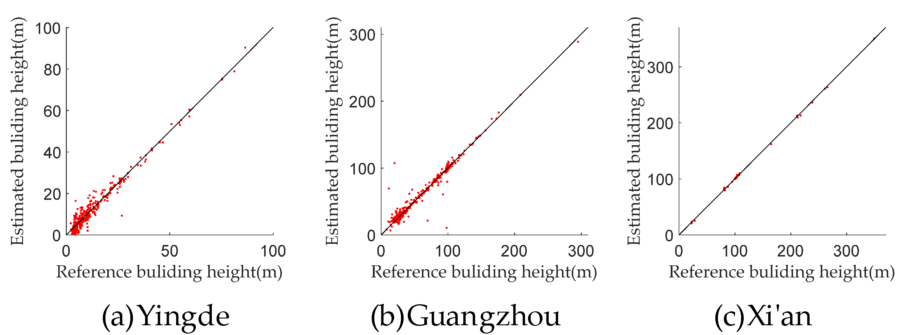
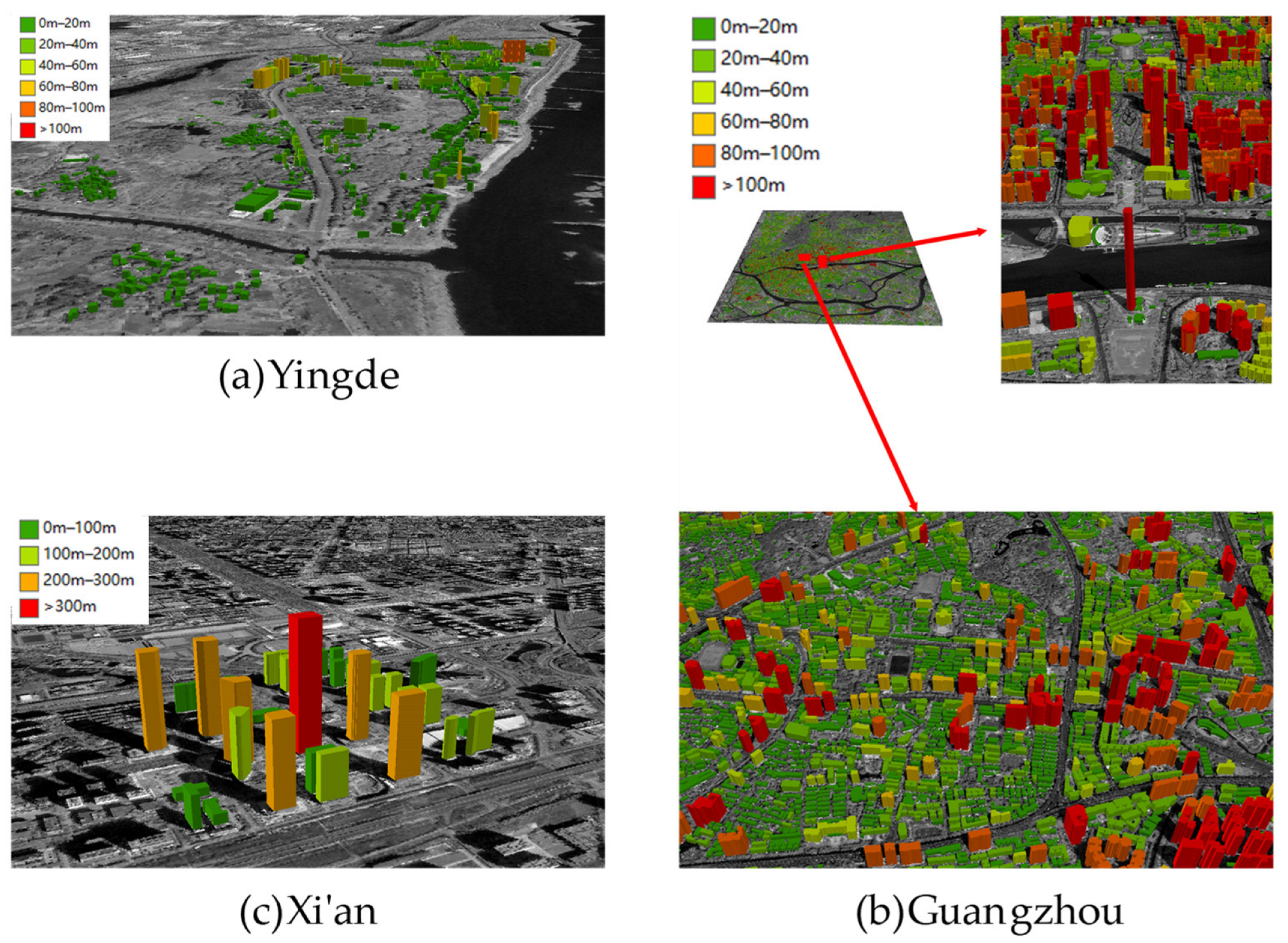
The evaluation result is shown in Figure 17. The MAE and RMSE for each group are calculated and presented in Table 1 below. The right-tailed, two-sample t-test was conducted to compare the MAEs. The results of the t-test are summarized in Table 2. Additionally, Figure 18 displays the 3D reconstruction models of buildings. According to the statistical results and significance testing, our algorithm performed worst in Guangzhou and best in Xi’an.
Our algorithm was implemented in C++ and ran on a desktop computer with an Intel Core i5-6500 processor clocked at 3.20 GHz, featuring four cores and four threads. The algorithm utilized OpenMP for parallelization to leverage multi-core processing capabilities. In Guangzhou’s experimental areas, contour matching processed 89,093 buildings in a total time of 11,191 s, while ground filtering processed the DSM with dimensions of 34,613 × 38,824 in a total time of 14,041 s.
3.4. Comparative Experiment
The building height extraction methods based on the GF-7 satellite image chosen for the comparison experiments are as follows:
- (1)
- The first comparison calculates building heights using the maximum and minimum elevations within the DSM within the building buffer zone [35], hereafter referred to as the ‘DSM method’.
- (2)
- In the second comparison, the ground elevation around the building is extracted by our algorithm, and the building rooftop elevation is extracted using the maximum elevations within DSM elevations within the building buffer zone, hereafter referred to as the ‘DSM + DEM method’.
- (3)
- Wang et al.’s method [30] was chosen as the third comparison, hereafter referred to as the ‘nDSM method’.
- (4)
- Zhang et al.’s method [26] was compared with ours, hereafter referred to as ‘Zhang’s method’.
Table 3 summarizes the accuracy of the comparative experiment. As Zhang’s algorithm cannot use building footprints as input data, we cite their experimental results in Xi’an [26] for comparison with ours. The right-tailed, two-sample t-test was conducted to compare the MAE of these methods. The results are summarized in Table 4. ME was used to reflect the distribution of errors in this comparative experiment, and the one-sample t-test was conducted to test whether errors followed a normal distribution with a mean of zero. Table 5 shows the result of the one-sample t-test. Figure 19 showcases the distribution of errors in building height extraction. The statistical analysis demonstrated that the building height extraction accuracy achieved by our algorithm outperformed comparative methods across all three study areas. The significance testing in Table 5 shows that the error distribution of the DSM method and DSM + DEM method did not have a mean equal to zero. This means that the building height extracted by these methods was higher than it actually was.
To make a comparison with Zhang’s method, the t-test for a hypothesized mean was conducted. The null hypothesis states that the absolute errors of our method came from a distribution with a mean of 1.69 m. The t-test yielded a t-value of −0.6928 with a corresponding p-value of 0.4933. This means that Zhang’s method demonstrated comparable accuracy to our algorithm in the Xi’an experimental area. However, our method can utilize building footprints as input data, making it more versatile in its application.
3.5. Ablation Experiment
To improve the performance of contour matching, this paper proposes two improvements: contour template correction based on the edges extracted on a backward image and local maximum values filtering by the DSM. The effect of improvements was examined in the ablation experiment. The following algorithms were used in ablation experiments:
- (1)
- Conventional contour matching algorithm [39], hereafter referred to as the ‘CM-C’.
- (2)
- Contour matching algorithm with contour template correction based on the edges extracted on backward image, hereafter referred to as the ‘CM-I’.
- (3)
- Contour matching algorithm with local maximum values filtering by the DSM, hereafter referred to as the ‘CM-D’.
In Yingde, the contour matching algorithm for the building footprint only includes the module that local maximum values filtering. Therefore, CM-C was performed for the ablation experiment. In Guangzhou, all methods were used for the ablation experiment. In Xi’an, due to the high precision of the building rooftop, there was no mismatch in the conventional contour matching method. Therefore, no ablation experiment was conducted.
According to the three-sigma rule of thumb, the thresholds for identifying mismatches were computed using the errors of our method. Table 6 presents the thresholds and the counts of matched buildings and mismatch. Figure 20 illustrates the distribution of absolute error in building heights. The experimental results demonstrate that our improvement can effectively reduce mismatches.
4. Discussion
4.1. Buildings of Different Heights
The building height extraction methods were compared on the buildings of different heights. The buildings were divided into three groups according to the reference height: below 20 m, between 20 and 100 m, and taller than 100 m. Table 7 provides a summary of the accuracy metrics. In Yingde, conventional methods exhibited poorer performance on buildings between 20 and 100 m compared to those below 20 m. Similarly, they fared worse on buildings taller than 100 m compared to those between 20 and 100 m in Guangzhou. This can be attributed to the disparity discontinuity issue encountered by dense matching algorithms.
In contrast, our proposed algorithm demonstrated superior performance on high-rise buildings relative to low-rise buildings. This was because low-rise buildings are more susceptible to occlusion, whereas high-rise buildings tend to have larger and more distinct features. As shown in Figure 21, there were instances of building loss in the DSM from stereo images for high-rise buildings exceeding 300 m. Nevertheless, our proposed algorithm is capable of matching building rooftops in such cases.
4.2. Building in Different Environments
In this paper, the error sources of the algorithm were analyzed in three zones with different environments. Figure 22 shows the three zones. ‘Zone 1’ is situated in the Xi’an experimental area, characterized by flat terrain and minimal vegetation. ‘Zone 2’ is located in the Guangzhou experiment area, featuring flat terrain but substantial occlusion by trees. ‘Zone 3’, also located in Guangzhou, exhibits occluded undulating terrain.
Table 8 summarizes the accuracy of rooftop elevation and ground elevation. According to the ME of rooftop elevation in the three zones, the roof elevation obtained from the DSM was higher than the actual value. The appendages on the rooftop, such as elevator rooms, stairwells, and water tanks, contributed to this discrepancy, as they were higher than the rooftop plane. This primarily accounts for the higher building height extracted by the DSM method in the comparison experiment. In contrast, our method extracts the elevation of the rooftop plane by matching the building rooftop. In applications such as per capita housing area estimation, considering the structural height as the building height becomes necessary. Our method is more suitable for addressing these cases.
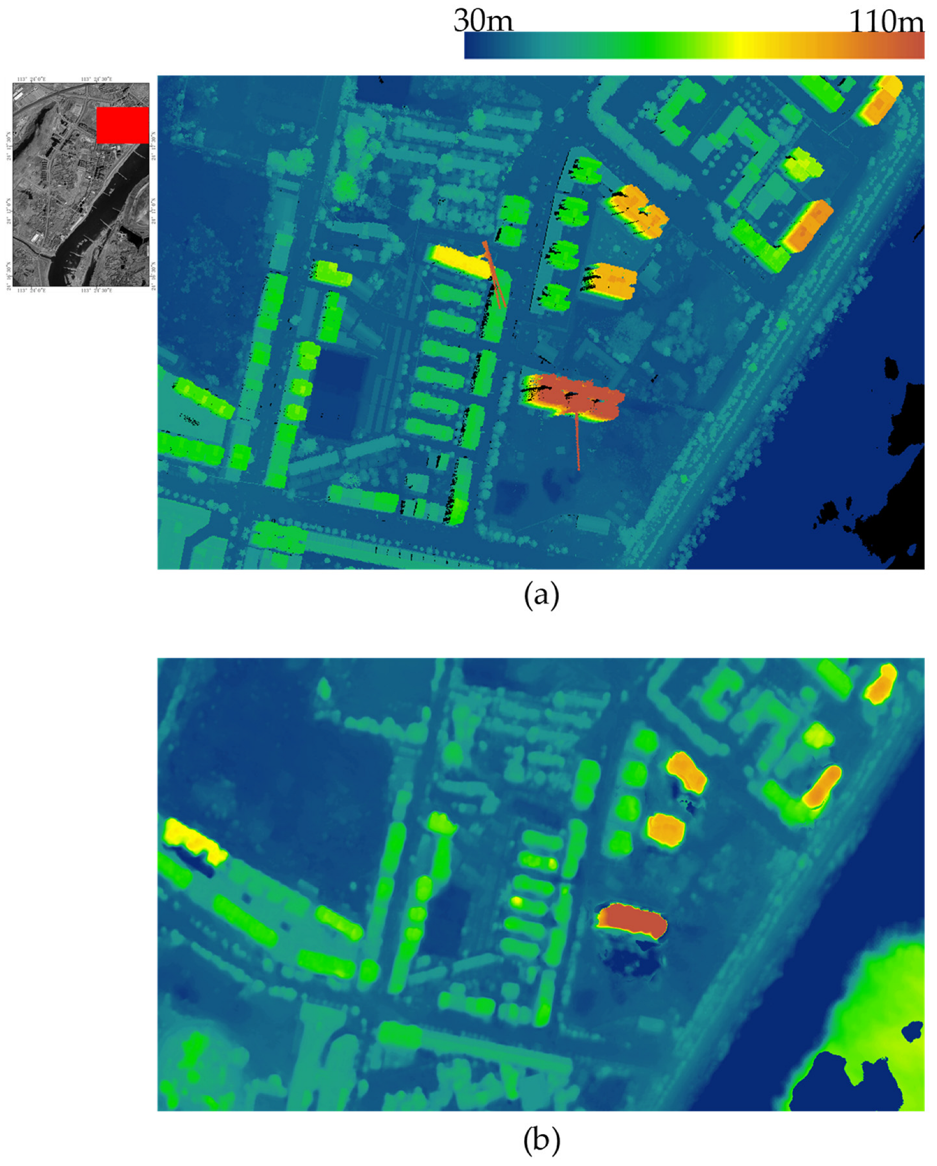
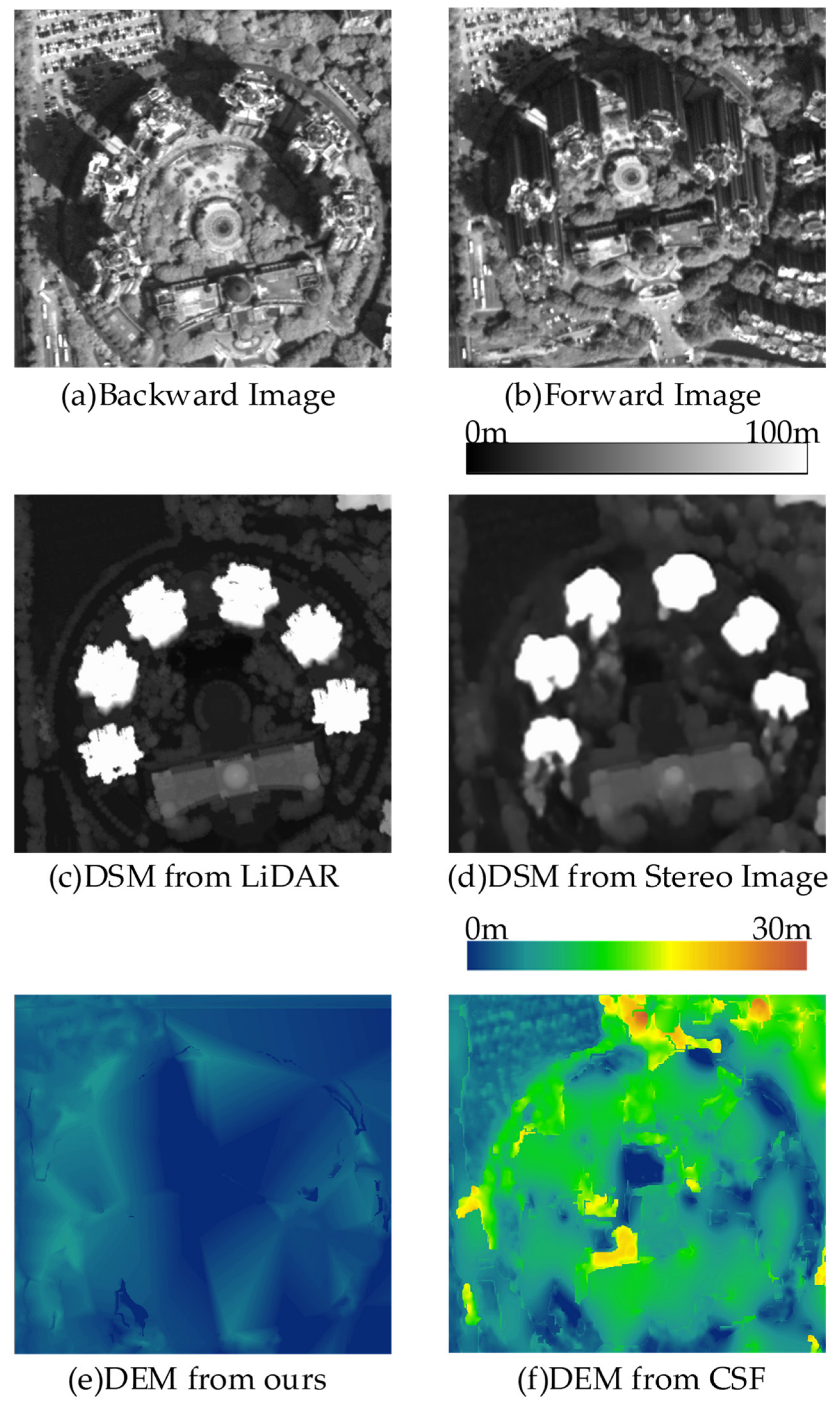
According to the ME of ground elevation, the ground elevation extracted by the nDSM method is higher than the actual value. As shown in Figure 6a, 3D breaklines were modeled as smooth transitions from the ground level to the building level. The smooth transitions were easily classified as ground points by the CSF algorithm, resulting in the DEM corresponding to the building location being higher than the surrounding ground. We eliminated inaccurate ground points around buildings, resulting in a more accurate ground elevation, as shown in Figure 23.
For traditional methods, the MEs of ground elevation in Zone 2 were larger than those in Zone 1. This indicates that the traditional method faces difficulty in extracting ground elevation in areas with high vegetation coverage. The proposed method uses image classification to ensure that the elevation of occluded ground is estimated from slightly distant ground points. It performs well on flat terrain such as Zone 2.
4.3. Limitation
Unclear building edges. Despite implementing two improvements, namely, contour template correction based on the edges extracted on the backward image and local maximum values filtering by the DSM, mismatches caused by unclear building edges remained in the Guangzhou experiment. To address this issue in future research, semantic segmentation can be used to exclude the edges that do not belong to building rooftops, and better edge extraction methods can also be used to extract more complete building edges for more accurate matching.
Occluded undulating terrain. As observed in the experimental results of Zone 3 in Section 4.2, obtaining ground elevation from the DSM in areas where undulating terrain is occluded by trees poses a significant challenge. To overcome this limitation, integrating additional data sources such as ground measurement data or other satellite images could offer a solution.
Pitched roof. As discussed in Section 4.2, the contour matching algorithm performed poorly in Zone 3, attributed to the presence of buildings with pitched roofs. Identification of pitched roofs is still a challenging task due to the limitations of image resolution. We aim to address this challenge in the future by leveraging higher resolution images.
5. Conclusions
This paper proposes a method for extracting building heights from high-resolution GF-7 stereo imagery. The method employs contour matching techniques to enhance building rooftop elevation extraction. Within the contour matching process, the method filters local maximum values by a DSM to resolve the mismatch issue. Moreover, the contour template correction is used to ensure higher precision in cases of unclear building edges. To improve the accuracy of the ground elevation extraction around the building, this method utilized image classification from the GF-7 multispectral imagery to identify and remove error-prone regions within the DSM, aiming to enhance the accuracy of ground filtering. The proposed method was validated in Yingde, Guangzhou, and Xi’an, showcasing its performance against comparative algorithms. The proposed method has more advantages for high-rise buildings. In the rooftop elevation extraction, the proposed algorithm takes the rooftop as an object, unaffected by issues such as smooth transitions in the DSM and rooftop appendages affecting the rooftop, resulting in more accurate results. In the ground elevation extraction, the proposed method effectively removes non-ground points and inaccurate ground points from the DSM, yielding accurate results in flat terrain.
However, problems such as unclear building edges and occluded undulating terrain are still challenges in building height extraction. In future research, semantic segmentation for identifying building edges and other data sources for ground elevation estimation can be considered to improve the accuracies of the elevation of rooftop and the ground elevation. Additionally, different satellite images from different cities, different countries, and even climate zones can be used to validate and improve the proposed methods.
Author Contributions
Conceptualization, Y.C., S.Z. and W.J.; methodology, Y.C. and W.J.; software, Y.C.; validation, Y.C.; formal analysis, Y.C.; investigation, Y.C.; resources, W.J.; data curation, Y.C.; writing—original draft preparation, Y.C.; writing—review and editing, G.Y.; visualization, Y.C. and S.Z.; supervision, S.Z.; project administration, S.Z.; funding acquisition, S.Z. All authors have read and agreed to the published version of the manuscript.
Funding
This work was supported by the High-Resolution Remote Sensing Application Demonstration System for Urban Fine Management under grant 06-Y30F04-9001-20/22.
Data Availability Statement
Data available on request due to restrictions. Our method is based on the original stereo images, which is restricted to be accessed on web according to the data policy of China, we are sorry that we cannot share our research data.
Conflicts of Interest
The authors declare no conflicts of interest.
References
- Mahtta, R.; Mahendra, A.; Seto, K.C. Building up or Spreading out? Typologies of Urban Growth across 478 Cities of 1 Million+. Environ. Res. Lett. 2019, 14, 124077. [Google Scholar] [CrossRef]
- Du, Y.; Mak, C.M.; Tang, B. Effects of Building Height and Porosity on Pedestrian Level Wind Comfort in a High-Density Urban Built Environment. Build. Simul. 2018, 11, 1215–1228. [Google Scholar] [CrossRef]
- Li, X.; Yang, B.; Liang, F.; Zhang, H.; Xu, Y.; Dong, Z. Modeling Urban Canopy Air Temperature at City-Block Scale Based on Urban 3D Morphology Parameters—A Study in Tianjin, North China. Build. Environ. 2023, 230, 110000. [Google Scholar] [CrossRef]
- Xu, S.; Li, G.; Zhang, H.; Xie, M.; Mendis, T.; Du, H. Effect of Block Morphology on Building Energy Consumption of Office Blocks: A Case of Wuhan, China. Buildings 2023, 13, 768. [Google Scholar] [CrossRef]
- Zhou, X.; Huang, Z.; Scheuer, B.; Wang, H.; Zhou, G.; Liu, Y. High-Resolution Estimation of Building Energy Consumption at the City Level. Energy 2023, 275, 127476. [Google Scholar] [CrossRef]
- Hang, J.; Li, Y.; Sandberg, M.; Buccolieri, R.; Di Sabatino, S. The Influence of Building Height Variability on Pollutant Dispersion and Pedestrian Ventilation in Idealized High-Rise Urban Areas. Build. Environ. 2012, 56, 346–360. [Google Scholar] [CrossRef]
- Kim, J.-W.; Baik, J.-J.; Park, S.-B.; Han, B.-S. Impacts of Building-Height Variability on Turbulent Coherent Structures and Pollutant Dispersion: Large-Eddy Simulations. Atmos. Pollut. Res. 2023, 14, 101736. [Google Scholar] [CrossRef]
- Zhang, X.; Liao, Q.; Yin, X.; Yin, Z.; Cao, Q. Spatial Characteristics and Influencing Factors of Multi-Scale Urban Living Space (ULS) Carbon Emissions in Tianjin, China. Buildings 2023, 13, 2393. [Google Scholar] [CrossRef]
- Lian, H.; Zhang, J.; Li, G.; Ren, R. The Relationship between Residential Block Forms and Building Carbon Emissions to Achieve Carbon Neutrality Goals: A Case Study of Wuhan, China. Sustainability 2023, 15, 15751. [Google Scholar] [CrossRef]
- Tosi, P.; De Rubeis, V.; Sbarra, P. Earthquake Perception Data Highlight Natural Frequency Details of Italian Buildings. Earthq. Spectra 2023, 39, 1240–1254. [Google Scholar] [CrossRef]
- Gui, S.; Qin, R. Automated LoD-2 Model Reconstruction from Very-High-Resolution Satellite-Derived Digital Surface Model and Orthophoto. ISPRS J. Photogramm. Remote Sens. 2021, 181, 1–19. [Google Scholar] [CrossRef]
- Baltsavias, E.P. A Comparison between Photogrammetry and Laser Scanning. ISPRS J. Photogramm. Remote Sens. 1999, 54, 83–94. [Google Scholar] [CrossRef]
- Sun, S.; Salvaggio, C. Aerial 3D Building Detection and Modeling From Airborne LiDAR Point Clouds. IEEE J. Sel. Top. Appl. Earth Obs. Remote Sens. 2013, 6, 1440–1449. [Google Scholar] [CrossRef]
- Lao, J.; Wang, C.; Zhu, X.; Xi, X.; Nie, S.; Wang, J.; Cheng, F.; Zhou, G. Retrieving Building Height in Urban Areas Using ICESat-2 Photon-Counting LiDAR Data. Int. J. Appl. Earth Obs. Geoinf. 2021, 104, 102596. [Google Scholar] [CrossRef]
- Zheng, Y.; Weng, Q. Model-Driven Reconstruction of 3-D Buildings Using LiDAR Data. IEEE Geosci. Remote Sens. Lett. 2015, 12, 1541–1545. [Google Scholar] [CrossRef]
- Li, X.; Zhou, Y.; Gong, P.; Seto, K.C.; Clinton, N. Developing a Method to Estimate Building Height from Sentinel-1 Data. Remote Sens. Environ. 2020, 240, 111705. [Google Scholar] [CrossRef]
- Esch, T.; Brzoska, E.; Dech, S.; Leutner, B.; Palacios-Lopez, D.; Metz-Marconcini, A.; Marconcini, M.; Roth, A.; Zeidler, J. World Settlement Footprint 3D—A First Three-Dimensional Survey of the Global Building Stock. Remote Sens. Environ. 2022, 270, 112877. [Google Scholar] [CrossRef]
- Dong, B.; Zheng, Q.; Lin, Y.; Chen, B.; Ye, Z.; Huang, C.; Tong, C.; Li, S.; Deng, J.; Wang, K. Integrating Physical Model-Based Features and Spatial Contextual Information to Estimate Building Height in Complex Urban Areas. Int. J. Appl. Earth Obs. Geoinf. 2024, 126, 103625. [Google Scholar] [CrossRef]
- Zhuang, D.; Zhang, L.; Zou, B. Interferometry Modeling and Model-Based Height Estimation for Buildings in Urban DSM Reconstruction Based on Interferometric Synthetic Aperture Radar Technology. J. Appl. Remote Sens. 2023, 17, 034508. [Google Scholar] [CrossRef]
- Sun, Y.; Hua, Y.; Mou, L.; Zhu, X.X. Large-Scale Building Height Estimation from Single VHR SAR Image Using Fully Convolutional Network and GIS Building Footprints. In Proceedings of the 2019 Joint Urban Remote Sensing Event (JURSE), Vannes, France, 22–24 May 2019; IEEE: Vannes, France, 2019; pp. 1–4. [Google Scholar]
- Izadi, M.; Saeedi, P. Three-Dimensional Polygonal Building Model Estimation From Single Satellite Images. IEEE Trans. Geosci. Remote Sens. 2012, 50, 2254–2272. [Google Scholar] [CrossRef]
- Lee, T.; Kim, T. Automatic Building Height Extraction by Volumetric Shadow Analysis of Monoscopic Imagery. Int. J. Remote Sens. 2013, 34, 5834–5850. [Google Scholar] [CrossRef]
- Qi, F.; Zhai, J.Z.; Dang, G. Building Height Estimation Using Google Earth. Energy Build. 2016, 118, 123–132. [Google Scholar] [CrossRef]
- Zhao, Y.; Wu, B.; Li, Q.; Yang, L.; Fan, H.; Wu, J.; Yu, B. Combining ICESat-2 Photons and Google Earth Satellite Images for Building Height Extraction. Int. J. Appl. Earth Obs. Geoinf. 2023, 117, 103213. [Google Scholar] [CrossRef]
- Zhang, H.; Xu, C.; Fan, Z.; Li, W.; Sun, K.; Li, D. Detection and Classification of Buildings by Height from Single Urban High-Resolution Remote Sensing Images. Appl. Sci. 2023, 13, 10729. [Google Scholar] [CrossRef]
- Zhang, C.; Cui, Y.; Zhu, Z.; Jiang, S.; Jiang, W. Building Height Extraction from GF-7 Satellite Images Based on Roof Contour Constrained Stereo Matching. Remote Sens. 2022, 14, 1566. [Google Scholar] [CrossRef]
- Liu, C.; Huang, X.; Wen, D.; Chen, H.; Gong, J. Assessing the Quality of Building Height Extraction from ZiYuan-3 Multi-View Imagery. Remote Sens. Lett. 2017, 8, 907–916. [Google Scholar] [CrossRef]
- Hirschmuller, H. Stereo Processing by Semiglobal Matching and Mutual Information. IEEE Trans. Pattern Anal. Mach. Intell. 2008, 30, 328–341. [Google Scholar] [CrossRef] [PubMed]
- Zhang, K.; Chen, S.-C.; Whitman, D.; Shyu, M.-L.; Yan, J.; Zhang, C. A Progressive Morphological Filter for Removing Nonground Measurements from Airborne LIDAR Data. IEEE Trans. Geosci. Remote Sens. 2003, 41, 872–882. [Google Scholar] [CrossRef]
- Wang, J.; Hu, X.; Meng, Q.; Zhang, L.; Wang, C.; Liu, X.; Zhao, M. Developing a Method to Extract Building 3D Information from GF-7 Data. Remote Sens. 2021, 13, 4532. [Google Scholar] [CrossRef]
- Zhang, W.; Qi, J.; Wan, P.; Wang, H.; Xie, D.; Wang, X.; Yan, G. An Easy-to-Use Airborne LiDAR Data Filtering Method Based on Cloth Simulation. Remote Sens. 2016, 8, 501. [Google Scholar] [CrossRef]
- He, S.; Zhou, R.; Li, S.; Jiang, S.; Jiang, W. Disparity Estimation of High-Resolution Remote Sensing Images with Dual-Scale Matching Network. Remote Sens. 2021, 13, 5050. [Google Scholar] [CrossRef]
- Laga, H.; Jospin, L.V.; Boussaid, F.; Bennamoun, M. A Survey on Deep Learning Techniques for Stereo-Based Depth Estimation. IEEE Trans. Pattern Anal. Mach. Intell. 2022, 44, 1738–1764. [Google Scholar] [CrossRef] [PubMed]
- Li, S.; He, S.; Jiang, S.; Jiang, W.; Zhang, L. WHU-Stereo: A Challenging Benchmark for Stereo Matching of High-Resolution Satellite Images. IEEE Trans. Geosci. Remote Sens. 2023, 61, 5603914. [Google Scholar] [CrossRef]
- Chen, P.; Huang, H.; Liu, J.; Wang, J.; Liu, C.; Zhang, N.; Su, M.; Zhang, D. Leveraging Chinese GaoFen-7 Imagery for High-Resolution Building Height Estimation in Multiple Cities. Remote Sens. Environ. 2023, 298, 113802. [Google Scholar] [CrossRef]
- Cao, Y.; Huang, X. A Deep Learning Method for Building Height Estimation Using High-Resolution Multi-View Imagery over Urban Areas: A Case Study of 42 Chinese Cities. Remote Sens. Environ. 2021, 264, 112590. [Google Scholar] [CrossRef]
- Perko, R.; Raggam, H.; Gutjahr, K.H.; Schardt, M. Advanced Dtm Generation from Very High Resolution Satellite Stereo Images. ISPRS Ann. Photogramm. Remote Sens. Spat. Inf. Sci. 2015, II-3/W4, 165–172. [Google Scholar] [CrossRef]
- Canny, J. A Computational Approach to Edge Detection. IEEE Trans. Pattern Anal. Mach. Intell. 1986, PAMI-8, 679–698. [Google Scholar] [CrossRef]
- Gong, J.; Hu, X.; Pang, S.; Wei, Y. Roof-Cut Guided Localization for Building Change Detection from Imagery and Footprint Map. Photogramm. Eng. Remote Sens. 2019, 85, 543–558. [Google Scholar] [CrossRef]
- Ebisch, K. A Correction to the Douglas–Peucker Line Generalization Algorithm. Comput. Geosci. 2002, 28, 995–997. [Google Scholar] [CrossRef]
- Huang, X.; Zhang, L. Morphological Building/Shadow Index for Building Extraction From High-Resolution Imagery Over Urban Areas. IEEE J. Sel. Top. Appl. Earth Obs. Remote Sens. 2012, 5, 12. [Google Scholar] [CrossRef]
- Zhang, J.; Lin, X. Filtering Airborne LiDAR Data by Embedding Smoothness-Constrained Segmentation in Progressive TIN Densification. ISPRS J. Photogramm. Remote Sens. 2013, 81, 44–59. [Google Scholar] [CrossRef]
Figure 1.
The problems faced in building heights extraction from the DSM. (a) Inaccuracies in the ground elevation; (b) Inaccuracies in high-rise buildings; (c) Occlusion caused by trees. (Left: buildings in the GF-7 backward images, middle: corresponding DSM for the buildings, right: inaccurate elevations in the DSM).

Figure 2.
Building height extraction workflow.

Figure 3.
Edge detection results and contour point directions (a) original image; (b) edge detection results; (c) contour point direction in conventional method; (d) contour point direction in our method.
Figure 3.
Edge detection results and contour point directions (a) original image; (b) edge detection results; (c) contour point direction in conventional method; (d) contour point direction in our method.

Figure 4.
Building contour template construction. (The colors in building contour template represent the weight of the contour point).
Figure 4.
Building contour template construction. (The colors in building contour template represent the weight of the contour point).

Figure 5.
The principle of building rooftop elevation extraction.

Figure 6.
Ground filtering algorithm. (a) Profile comparisons of DSMs from LiDAR and the stereo image. (b) The way of searching inaccurate ground points. (c) Multispectral image. (d) Inaccurate points. (e) Input DSM. (f) Generated DEM.
Figure 6.
Ground filtering algorithm. (a) Profile comparisons of DSMs from LiDAR and the stereo image. (b) The way of searching inaccurate ground points. (c) Multispectral image. (d) Inaccurate points. (e) Input DSM. (f) Generated DEM.

Figure 7.
The building rooftop contours with multiple elevations and their matched edges. The red edges in the image indicate matched edges. (a) The building rooftop contour encompassing the podium building. (c) The building rooftop contour encompassing the building side. (b,d) The contour matching results in the forward image.

Figure 8.
Building contour segmentation process. (a) The and ; (b) Samples of the main building rooftop; (c) Samples of the podium building; (d) Initial main building rooftop; (e) Main building rooftop; (f) Result of segmentation.
Figure 8.
Building contour segmentation process. (a) The and ; (b) Samples of the main building rooftop; (c) Samples of the podium building; (d) Initial main building rooftop; (e) Main building rooftop; (f) Result of segmentation.

Figure 9.
Building contour segmentation results. (a) The known building contours, where the red edges indicate matched edges. (b) The contour matching results, where the red edges indicate . (c) The samples of the main building rooftop. (d) The main building rooftop extracted by our method. (e) The contour matching results after segmentation.

Figure 10.
The images and building footprints of the Yingde experimental area. (a) The backward image, (b) the forward image, and (c) the building footprints.
Figure 10.
The images and building footprints of the Yingde experimental area. (a) The backward image, (b) the forward image, and (c) the building footprints.

Figure 11.
The DSM of Yingde experimental area. (a) The DSM obtained from the LiDAR data, with a spatial resolution of 1 m; (b) the DSM generated from the GF-7 stereo images.
Figure 11.
The DSM of Yingde experimental area. (a) The DSM obtained from the LiDAR data, with a spatial resolution of 1 m; (b) the DSM generated from the GF-7 stereo images.

Figure 12.
The GF-7 image of the Guangzhou experimental area. (a) The backward image; (b) the forward image.
Figure 12.
The GF-7 image of the Guangzhou experimental area. (a) The backward image; (b) the forward image.

Figure 13.
A portion of building rooftop contours and the DSM in the Guangzhou experimental area. (a) The DSM obtained from the LiDAR data, with a spatial resolution of 1 m; (b) the DSM generated from the GF-7 stereo images; (c) the building rooftop contours.
Figure 13.
A portion of building rooftop contours and the DSM in the Guangzhou experimental area. (a) The DSM obtained from the LiDAR data, with a spatial resolution of 1 m; (b) the DSM generated from the GF-7 stereo images; (c) the building rooftop contours.

Figure 14.
The Xi’an experimental area. (a) The backward image and building rooftop contours; (b) the forward image; (c) the DSM generated from the GF-7 stereo images.
Figure 14.
The Xi’an experimental area. (a) The backward image and building rooftop contours; (b) the forward image; (c) the DSM generated from the GF-7 stereo images.

Figure 15.
The distribution of reference building height. (a) Yingde; (b) Guangzhou; (c) Xi’an.

Figure 16.
The factors influencing contour matching in the Yingde and Guangzhou experimental areas.

Figure 17.
The building height extraction results of our algorithm.

Figure 18.
Three-dimensional reconstruction models of buildings.

Figure 19.
Distribution of building height extraction errors in comparative experiments. (The contour matching algorithm for the building footprint is referred to as the ‘CM-F’; the contour matching algorithm for building rooftop contour is referred to as the ‘CM-R’).
Figure 19.
Distribution of building height extraction errors in comparative experiments. (The contour matching algorithm for the building footprint is referred to as the ‘CM-F’; the contour matching algorithm for building rooftop contour is referred to as the ‘CM-R’).

Figure 20.
Distribution of building height extraction errors in the ablation experiment.

Figure 21.
Examples of buildings above 300 m in the Guangzhou experimental area.

Figure 22.
The zones with different environments.

Figure 23.
Comparison of ground filtering algorithms.


Table 1.
Accuracy statistics of our method.
| MAE (m) | RMSE (m) | |
|---|---|---|
| Yingde | 1.96 | 2.68 |
| Guangzhou | 3.76 | 7.60 |
| Xi’an | 1.55 | 1.93 |
Table 2.
Results of right-tailed, two-sample t-test for the proposed algorithm.
| Test Case | t | p | |
|---|---|---|---|
| Guangzhou | Yingde | 3.5637 | 0.0002 |
| Guangzhou | Xi’an | 4.2637 | 0.0000 |
| Yingde | Xi’an | 1.8538 | 0.0348 |
Note: 1. For the first row, the null hypothesis states that there is no difference in MAE between the two groups, while the alternative hypothesis suggests that the MAE of the below 20 m group is greater than the MAE of the 20–100 m group. 2. The significance level for all tests was set at 5%.
Table 3.
Accuracy statistics of building height extraction in the comparative experiment.
| Yingde | Guangzhou | Xi’an | |||||||
|---|---|---|---|---|---|---|---|---|---|
| ME (m) | MAE (m) | RMSE (m) | ME (m) | MAE (m) | RMSE (m) | ME (m) | MAE (m) | RMSE (m) | |
| DSM | 4.48 | 4.84 | 7.52 | 6.19 | 6.69 | 10.92 | 6.74 | 7.00 | 8.56 |
| DSM + DEM | 4.01 | 4.35 | 6.70 | 4.84 | 5.40 | 9.78 | 3.85 | 4.85 | 5.24 |
| nDSM | 3.99 | 4.33 | 5.47 | 0.35 | 4.32 | 8.65 | 0.86 | 4.40 | 6.17 |
| Zhang | - | - | - | - | - | - | - | 1.69 | 2.23 |
| Ours | −0.32 | 1.96 | 2.68 | 0.22 | 3.76 | 7.60 | −0.15 | 1.55 | 1.93 |
Table 4.
Results of right-tailed, two-sample t-test for the comparative experiment.
| Test Case | t | p | ||
|---|---|---|---|---|
| Yingde | DSM | Ours | 8.8137 | 0.0000 |
| DSM + DEM | Ours | 8.1771 | 0.0000 | |
| nDSM | Ours | 11.4755 | 0.0000 | |
| DSM | DSM + DEM | 1.1702 | 0.1212 | |
| Guangzhou | DSM | Ours | 7.2432 | 0.0000 |
| DSM + DEM | Ours | 4.8014 | 0.0000 | |
| nDSM | Ours | 2.6618 | 0.0039 | |
| DSM | DSM + DEM | 2.4266 | 0.0077 | |
| Xi’an | DSM | Ours | 6.1901 | 0.0000 |
| DSM + DEM | Ours | 5.1362 | 0.0000 | |
| nDSM | Ours | 3.6606 | 0.0004 | |
| DSM | DSM + DEM | 2.6572 | 0.0052 | |
Note: 1. For the first row, the null hypothesis states that there is no difference in MAE between the two groups, while the alternative hypothesis suggests that the MAE of the DSM method is greater than the MAE of our method. 2. The significance level for all tests was set at 5%.
Table 5.
Results of one-sample t-test for error distributions.
| Test Case | t | p | |
|---|---|---|---|
| Yingde | DSM | 13.7416 | 0.0000 |
| DSM + DEM | 13.8075 | 0.0000 | |
| nDSM | 19.7254 | 0.0000 | |
| Ours | −2.2283 | 0.0265 | |
| Guangzhou | DSM | 15.4601 | 0.0000 |
| DSM + DEM | 12.7919 | 0.0000 | |
| nDSM | 0.9139 | 0.3612 | |
| Ours | 0.6516 | 0.5150 | |
| Xi’an | DSM | 7.3354 | 0.0000 |
| DSM + DEM | 6.2139 | 0.0000 | |
| nDSM | 0.8068 | 0.4255 | |
| Ours | −0.4548 | 0.6515 |
Note: 1. For the first row, the null hypothesis states that the errors of the DSM method come from a normal distribution with a mean equal to zero and unknown variance, while the alternative hypothesis suggests that the error distribution does not have a mean equal to zero. 2. The significance level for all tests was set at 5%.
Table 6.
Accuracy statistics of building height extraction in the ablation experiment.
| Yingde (343 Buildings) | Guangzhou (506 Buildings) | |||||
|---|---|---|---|---|---|---|
| ) | Mismatch | Mismatch | ||||
| CM-C | 6.70 | 242 | 101 | 7.93 | 368 | 138 |
| CM-I | - | - | 425 | 81 | ||
| CM-D | - | - | 467 | 39 | ||
| CM-F | 336 | 7 | - | - | ||
| CM-R | - | - | 476 | 30 | ||
Note: The contour matching algorithm for the building footprint is referred to as the ‘CM-F’. The contour matching algorithm for the building rooftop contour is referred to as the ‘CM-R’.
Table 7.
Accuracy statistics of buildings with different heights.
| Number | MAE (m) | RMSE (m) | |||
|---|---|---|---|---|---|
| Yingde | <20 m | 287 | ours | 2.03 | 2.63 |
| DSM | 4.60 | 7.35 | |||
| DSM + DEM | 4.33 | 6.74 | |||
| nDSM | 4.27 | 5.49 | |||
| 20–100 m | 56 | ours | 1.63 | 2.94 | |
| DSM | 6.08 | 8.31 | |||
| DSM + DEM | 4.49 | 6.49 | |||
| nDSM | 4.62 | 5.40 | |||
| ≥100 m | 0 | - | - | ||
| Guangzhou | <20 m | 28 | ours | 5.98 | 12.07 |
| DSM | 14.72 | 22.71 | |||
| DSM + DEM | 13.42 | 21.67 | |||
| nDSM | 9.29 | 17.63 | |||
| 20–100 m | 429 | ours | 3.01 | 7.57 | |
| DSM | 5.72 | 9.55 | |||
| DSM + DEM | 4.74 | 8.67 | |||
| nDSM | 3.86 | 7.94 | |||
| ≥100 m | 49 | ours | 2.45 | 3.31 | |
| DSM | 10.56 | 11.77 | |||
| DSM + DEM | 6.65 | 7.82 | |||
| nDSM | 5.57 | 6.51 | |||
| Xi’an | <20 m | 0 | - | - | |
| 20–100 m | 14 | ours | 1.57 | 1.95 | |
| DSM | 7.21 | 8.49 | |||
| DSM + DEM | 4.18 | 4.45 | |||
| nDSM | 5.80 | 8.06 | |||
| ≥100 m | 20 | ours | 1.54 | 1.92 | |
| DSM | 6.85 | 8.60 | |||
| DSM + DEM | 3.37 | 5.73 | |||
| nDSM | 3.42 | 4.37 |
Table 8.
Accuracy statistics of buildings with different environments.
| Number | Rooftop Elevation | Ground Elevation | ||||||
|---|---|---|---|---|---|---|---|---|
| ME (m) | MAE (m) | RMSE (m) | ME (m) | MAE (m) | RMSE (m) | |||
| Zone 1 | 34 | ours | −0.07 | 1.15 | 1.42 | 0.08 | 1.46 | 1.86 |
| DSM | 3.93 | 4.11 | 5.07 | −2.81 | 3.53 | 4.83 | ||
| nDSM | 2.42 | 3.58 | 4.67 | 1.56 | 3.52 | 4.84 | ||
| Zone 2 | 42 | ours | −0.33 | 0.74 | 1.16 | −0.40 | 1.49 | 2.09 |
| DSM | 6.84 | 6.84 | 9.00 | 2.15 | 3.41 | 4.73 | ||
| nDSM | 3.31 | 3.46 | 4.16 | 6.54 | 6.54 | 7.23 | ||
| Zone 3 | 30 | ours | −1.82 | 1.99 | 2.73 | −3.26 | 3.80 | 5.60 |
| DSM | 2.96 | 3.04 | 3.28 | −0.90 | 1.18 | 1.58 | ||
| nDSM | 2.24 | 2.71 | 3.06 | 2.75 | 2.75 | 3.08 | ||
Disclaimer/Publisher’s Note: The statements, opinions and data contained in all publications are solely those of the individual author(s) and contributor(s) and not of MDPI and/or the editor(s). MDPI and/or the editor(s) disclaim responsibility for any injury to people or property resulting from any ideas, methods, instructions or products referred to in the content. |
© 2024 by the authors. Licensee MDPI, Basel, Switzerland. This article is an open access article distributed under the terms and conditions of the Creative Commons Attribution (CC BY) license (https://creativecommons.org/licenses/by/4.0/).
Share and Cite
MDPI and ACS Style
Cui, Y.; Zhao, S.; Jiang, W.; Yu, G. Urban Building Height Extraction from Gaofen-7 Stereo Satellite Images Enhanced by Contour Matching. Remote Sens. 2024, 16, 1556. https://doi.org/10.3390/rs16091556
AMA Style
Cui Y, Zhao S, Jiang W, Yu G. Urban Building Height Extraction from Gaofen-7 Stereo Satellite Images Enhanced by Contour Matching. Remote Sensing. 2024; 16(9):1556. https://doi.org/10.3390/rs16091556
Chicago/Turabian StyleCui, Yunfan, Shuangming Zhao, Wanshou Jiang, and Guorong Yu. 2024. "Urban Building Height Extraction from Gaofen-7 Stereo Satellite Images Enhanced by Contour Matching" Remote Sensing 16, no. 9: 1556. https://doi.org/10.3390/rs16091556
Note that from the first issue of 2016, this journal uses article numbers instead of page numbers. See further details here.