

Robust Velocity Dealiasing for Weather Radar Based on Convolutional Neural Networks


1
Advanced Radar Research Center, University of Oklahoma, Norman, OK 73019, USA
2
School of Electrical and Computer Engineering, University of Oklahoma, Norman, OK 73019, USA
*
Author to whom correspondence should be addressed.
Remote Sens. 2023, 15(3), 802; https://doi.org/10.3390/rs15030802
Submission received: 24 December 2022
/
Revised: 22 January 2023
/
Accepted: 29 January 2023
/
Published: 31 January 2023
(This article belongs to the Topic Radar Signal and Data Processing with Applications)
(This article belongs to the Section AI Remote Sensing)
(This article belongs to the Section AI Remote Sensing)
Abstract
:Doppler weather radar is an essential tool for monitoring and warning of hazardous weather phenomena. A large aliasing range () is important for surveillance but a high aliasing velocity () is also important to obtain storm dynamics unambiguously. However, the and are inversely related to pulse repetition time. This “Doppler dilemma” is more challenging at shorter wavelengths. The proposed algorithm employs a CNN (convolutional neural network), which is widely used in image classification, to tackle the velocity dealiasing issue. Velocity aliasing can be converted to a classification problem. The velocity field and aliased count can be regarded as the input image and the label, respectively. Through a fit-and-adjust process, the best weights and the biases of the model are determined to minimize a cost function. The proposed method is compared against the traditional region-based method. Both methods show similar performance on mostly filled precipitation. For sparsely filled precipitation; however, the CNN demonstrated better performance since the CNN processes the entire scan at once while the region-based method processes only the limited adjacent area.
1. Introduction
The Doppler weather radar is an essential tool for nowcasting, warning of severe storms and hazardous weather phenomena such as thunderstorms, blizzards, and hail [1]. For pulsed weather radars, a long aliasing range (), also known as the maximum unambiguous range, is desirable for surveillance. In direct conflict with this desire, a high aliasing velocity , also known as the Nyquist velocity, is essential to obtaining storm dynamics. The Doppler dilemma is the manifestation of this conflict—a long-lasting challenge where and are in a fixed trade-off relation [1]. The Doppler dilemma becomes more severe for shorter-wavelength radars such as the X-band compared to C- and S-band. Many efforts have been attempted to mitigate the Doppler dilemma (e.g., [2,3,4,5,6,7]). Because the performance of automated dealiasing algorithms can be poor at critical locations in a sweep, labor-intensive manual dealiasing is still being practiced (e.g., [8,9,10]). For that reason, an automated algorithm is still an important area of study, which is the primary motivation of the current work.
The Doppler dilemma can be derived as shown in Equation (1).
For a specific combination of and , the Doppler dilemma dictates the value. There are two common approaches to dealias the velocity measurements, which are (1) the post-processing method and (2) the waveform design method. In the first approach, aliased velocities are found by searching for velocity discontinuities (typically , where n is −2, −1, 1, 2, and so on). Subsequently, dealiasing is accomplished by adding/subtracting to the aliased velocities. One assumption is that the initial velocity measurement, e.g., first cell, first range gate, first azimuth, etc., is non-aliased. The velocity measurement of this cell is also known as the reference velocity, and there have been numerous attempts to determine the discontinuity [2,3,4,5,6,7]. In the second approach, two (or more) PRT values are used, and the aliased velocities are found by searching for disagreements between the two measurements. The approach is known as the dual-PRF method [1,11]. Dealiasing is accomplished with the waveform design approaches by solving a least-common-multiplier problem. There is a similar method known as the staggered PRT (Pulse Repetition Time) [12,13]. Both methods use two pulse repetition frequencies (or periods). The key difference is how the periods are arranged. The dual-PRF method collects a radial by splitting it into two halves; one half uses one period while the other half uses the other. The staggered-PRT method, however, collects a radial by staggering the two periods; hence the name staggered PRT [14,15,16,17,18].
It must be emphasized that the post-processing method allows the system to operate everything else, e.g., ground clutter filter, contiguous pulse-pair processing, etc., as is. The waveform design methods require modifications to the existing ground clutter filters due to the dwell discontinuity [17]. In this work, the main focus will be on the post-processing approach, and the key is to detect the aliasing. Once detected successfully, it can be dealiased correctly [2,3,4,19].
The detection of velocity aliasing is comparable to classification and one can see how a machine learning (ML) algorithm can be applied to mitigate velocity aliasing. In principle, a classification ML algorithm to determine how many times the velocity aliasing has occurred allows us to identify the regions where velocity dealiasing is necessary. In essence, the ML processing replaces what human intervention often is needed, i.e., identification of the velocity aliasing region and classification of the velocity aliasing count. ML can perform these two tasks in one pass, much like what a human is capable of. ML is a data-fitting method. In ML, model parameters, i.e., weights and biases, are optimized through an iterative training process. Optimization is performed to minimize a cost function. Each couple of weights and biases is a neuron, and multiple neurons form a neural network (1 layer). Neural networks that contain more than one layer are considered deep neural networks. Deep learning is the training process of deep neural networks [20]. A single-layer neural network is similar to the current technique (one threshold); however, the deep neural network is more complex, with the promise of better performance.
Image segmentation is performed through a CNN (Convolutional Neural Network); here, concatenated layers of filters operate like convolution. CNN-based image classification can produce a single label that represents the whole image, e.g., facial recognition [21], or an output image that indicates multiple labels (segments) within an image, e.g., medical diagnosis [22], object recognition, and so on. It is also applied in meteorological data processing, e.g., to classify spatially localized climate patterns from Community Atmospheric Model v5 (CAM5) simulation [23], to detect the cold and warm fronts from the reanalysis data [24], to classify the tropical cyclone intensity from satellite images [25], to predict the probability of severe hail [26], and to detect the birds roosts from combined radar products [27]. Like these examples, a CNN segments and labels the images. In this work, the label represents whether a velocity cell is aliased. The input is the raw velocity field, and the output is a map of flags indicating whether the velocity of a cell is aliased and, by extension, how many times the velocity is aliased. Therefore, aliasing detection can be converted into a labeling problem.
Our training goal is to encourage the model to learn the aliasing concept, rather than to memorize a set of patterns. It is important to provide a diverse set of data that cover most scenarios, e.g., Nyquist velocity, local mean velocity, storm pattern, scan elevation, etc. Just like how a human can dealias a velocity map regardless of these variables, the goal is to produce a CNN model that is capable of identifying aliasing count regardless of these variables. To that end, some high-level features, such as segments and abrupt changes of Doppler velocity are used to identify regions of aliasing.
The evaluation of velocity dealiasing performance is commonly performed by calculating the accuracy or error rate (1 − accuracy). Some studies calculate the error rate based on the error-included scan [2,28,29] and some studies evaluated the error rate based on error gates [19,30]. Case studies are also performed by analyzing specific PPI (Plan Position Indicator of one elevation angle) scans [6,19,28,29,30]. In this study, the mean of accuracy () and the standard deviation of accuracy () averaged by scans are employed to evaluate the performance. The indicates the consistency of performance. For example, a low with low means poor performance most of the time. However, a high with high means performance can vary widely and there are times the performance is unacceptable.
The overarching goal of this work is to exploit CNN for velocity dealiasing (aliasing detection/classification/labeling). This is a post-processing approach since even dual-PRF or staggered-PRT methods resulted in aliased velocity. The promise of using a CNN is to achieve human-level performance. Through this process, it is expected that the labor-intensive task of velocity dealiasing could be automated.
This paper is organized as follows. Section 2 describes the background, materials, and proposed methodology, including the data pre-processing, algorithm description, and training. Then, Section 3 explains the evaluation method and statistical results, presents an analysis of the sensitivity test of a selection of values and template sizes, and analyzes with specific examples. In Section 4, the limitations and future works will be discussed, and the conclusions of this paper are in Section 5.
2. Materials and Methods
2.1. Brief Review of Existing Techniques
Many attempts have been made to dealias Doppler velocity measurements. It started from a one-dimensional dealiasing, which checks the continuity along the radial [2] using the first meaningful range gate as the reference velocity. The key assumption is that the reference velocity is non-aliased. However, this assumption can be incorrect, which leads to error propagation. Later, the environmental wind, such as sounding, was introduced to aid the detection of aliasing [3]. It is especially beneficial for identifying whether an isolated storm is aliased. However, the wind profile from radiosonde could be significantly different in time and space, thus resulting in poor performance when the wind field is non-uniform and changes rapidly. For these reasons, the wind profile obtained by the Velocity Azimuth Display (VAD) was proposed to represent the environmental wind field [5,31,32]. The technique was subsequently extended to two or higher dimensional dealiasing methods [4,19]. These were introduced to improve the dealiasing performance since these methods take advantage of the neighboring cells in azimuth, elevation, and time. A four-dimensional dealiasing method that mitigates the issue of high dependency on external data sources such as sounding was introduced [28]. It uses the dealiased higher elevation angular velocity in the vertical dimension since operational radars usually utilize higher PRF values at higher scans and the former dealiased radar volume as initial reference velocity. The method proposed by [6] utilizes a two-dimensional multi-pass scheme, which checks the spatial discontinuity and dealiases the velocity by searching the reference velocity in two directions, i.e., clockwise and counterclockwise. It does not require external reference velocity data; instead, it has strict criteria for the first dealiasing of not complex precipitation such as stratiform, and gradually relieves the threshold to dealias the more complex velocities, including isolated storms. In the data assimilation field, a dealiasing scheme by using three-dimensional wind from VDRAS (Variational Doppler Radar Analysis System) as reference velocity was introduced by [29]. Most of the velocity dealiasing algorithms focus on typical storms with measured velocity ranging from 20 to 36 , and they are limited when the velocity is extremely strong, such as winds due to typhoons and hurricanes. Later, the ADTH (Automated Dealiasing for Typhoon and Hurricane) was developed [33]. It finds the first reference radial based on the local minima of GVAD (Gradient VAD) and a higher number of valid gates. Then, a two-way (clockwise and counterclockwise) and two directions (in azimuth and radial direction) continuity check is performed.
One popular radar processing software library, Py-ART (Python ARM Radar Toolkit), incorporates a novel region-based velocity dealiasing algorithm [7]. The key assumption of this method is that the first-guess field is non-aliased. Once the first-guess field is determined, it checks the adjacent radar cells for abrupt velocity changes within a storm cluster and, if aliased, dealiases the velocity by adding to the measurement. If a radar scan has multiple isolated storms, it produces multiple first-guess fields and processes each storm individually. If the assumption of the first-guess field is incorrect, it leads to incorrect velocity dealiasing of the connected storm.
The detection of velocity aliasing can be converted to a classification problem, and CNN is widely used in image classification. CNN is a collection of concatenated two-dimensional filters. To have the same output size as input, a U-Net architectured semantic segmentation using a CNN [34], which can recover the same output size by the de-convolution process, is employed as the model design. In the encoding process, input velocity is ingested, and it is processed into multiple levels of feature representations to keep the essence of velocity aliasing labeling. In the decoding process, a map of labels is generated from features learned by the encoder (lower resolution) to the pixel level (higher resolution). Besides the convolution with two-dimensional filters, there are downsampling and upsampling processes, known as the pooling layer for downsampling and de-convolution for upsampling. The convolutional layer convolves with internal 2-D filters to extract the features, and the downsampling layer lowers the resolution but keeps the essence of the features. Upsampling is used to recover the output size as the input size. In the context of U-Net, upsampling using an output along with the input from the previous layers at the same depth provides a mechanism to generate a feature map of the same size at the same depth. The last layer turns the output from the last de-convolutional layer into labels through a process that is similar to the mode process, i.e., the value at which the probability is the highest. A so-called softmax classifier is used in this step. A softmax function provides a normalized output, which can be used as the probability of each label. Therefore, it is commonly employed for multi-label classification [35]. The image segmentation process provides an output image of labels that indicate whether a velocity pixel is aliased.
2.2. Data Generation
Artificial aliasing based on S-band data is performed to generate the input velocity fields for training the CNN model. In this work, a simulated X-band radar velocity field is used as the input () to the CNN model. The X-band velocity is generated based on a set of simple rules and it includes the number of times the velocity has aliased, referred to as aliased count label (L) hereinafter. In the context of this study, is produced according to the following rules:
In short, can be defined as the following equation.
where the is the ground truth. For example, if , and , then and since it is once aliased in the positive direction. If , and , then and since it is twice aliased in the negative direction.
The training dataset is employed to update the model parameters, which are comprised of weights and biases. A validation dataset is used to determine the training stopping point, which is to protect the model from overfitting the training dataset. A test dataset is utilized to evaluate the performance, and these three datasets are mutually exclusive.
The number of scans for each dataset is shown in Table 1. In Table 1, scans from four different years and five different NEXRAD radar sites are collected to diversify the datasets. Furthermore, data are collected by considering the area where precipitation fills the scan. Although a qualitative categorization, the cases are separated into “mostly filled” precipitation and “sparsely filled” precipitation. Generally, these cases correspond to stratiform and convective precipitation, respectively. The training dataset consists of 1872 scans, which includes 624 cases from three elevation angles, i.e., 0.5°, 0.9°, and 1.3°. It comprises 240 scans of mostly filled precipitation and 1632 scans of sparsely filled precipitation. Unaliased velocity fields from the NEXRAD KTLX, KFWS, KICT, KLSX, and KLOT radar sites in 2018 are employed as the training dataset. The validation dataset includes 315 scans with 75 scans of mostly filled precipitation and 240 scans of sparsely filled precipitation (105 cases with three elevation angles), and the scans from the NEXRAD KTLX radar site in 2019 are collected. The test dataset has a total of 495 scans with 102 scans of mostly filled precipitation and 393 scans of sparsely filled precipitation, which is 135 cases with three elevation angles, and the scans were collected from the NEXRAD KTLX radar site in 2017 and 2020.
The mostly filled precipitation cases are characterized by being spatially continuous and having relatively simple features, which means the features can be trained with a lower number of scans. On the other hand, the sparsely filled precipitation is more complex and includes spatially discontinuous storms, which requires diverse training data to represent the complex features.
2.3. Proposed Algorithm
In this section, pre-processing and post-processing methods will be discussed. Velocity dealiasing issues will be converted to the detection of labeling problems and then measured velocity fields will be dealiased using the labels.
2.3.1. Pre-Processing
Input data are generated by considering a typical X-band radar coverage, which is approximately [36,37,38]. Since our collected training data are approximately 2000 scans, there is an inherent limitation of the training data size compared to other training data. Because of this, additional training data was generated by data augmentation, which diversified the datasets by slightly modified copies of existing data [39].
The typical size of the CNN model input data is defined as width by height by depth, where the width by height determines the two-dimensional image size, and the depth is the number of color channels such as the red, green, and blue components of an image. Concerning velocity dealiasing, the depth is one as the velocity is processed alone. The dimension D of the input array of the velocity is
where is the number of azimuths, and is the number of range gates. The output array shares the same dimension as the input array to predict the label at each gate.
With the NEXRAD range resolution of , 256 range gates are employed with a range coverage of to cover the aforementioned 60 range. The is re-sampled by a 2° spacing with 180 radials resulting in a full 360° coverage. The input array is expanded to 256 azimuths by copying the adjacent azimuths to produce a continuous input field, i.e., consists of azimuths 284, 286, …, 358, 0, 2, 4, …, 358, 0, 2, …, 74. For the aliased label prediction, the middle portion, i.e., azimuths 0, 2, 4, …, 358, is extracted as the final output.
The wind direction is inherently biased as the collected dataset is limited, and selected NEXRAD radars are located where there is a non-zero mean of the wind in terms of climate [40]. Since it could result in a CNN model having a directional bias, data augmentation is performed by randomly rotating the radar scans and negating the velocity values. That way, the mean wind is randomized and removed as a whole to train the CNN model. Input velocity () is a normalized unit. It is obtained by dividing the raw velocity by the to eliminate the bias and to map the input velocity to a range that is independent of specific values. In this study, a set of 60 rotation angles is used. Together with negating the sign, a 120-fold increase in the dataset is accomplished. However, this is by no means equivalent to replacing the dataset with a 120-fold larger collection but simply, as mentioned before, a practice to remove the non-zero mean and the directional distribution that are inherent in the dataset.
2.3.2. Training
Training is conducted with the internal model parameters, i.e., weights and biases, to minimize the loss through the fit-and-adjust process, which is also known as the gradient-descent algorithm. By concatenating a set of gradient descent through multiple layers, this process is referred to as the back propagation [35].
Cross-entropy is employed as a cost function, which is shown in the following:
where L is the true label, i represents the aliasing label, k is the cell index, and represents the output of the softmax classifier, which is shown in the following:
where M is the number of labels.
Intuitively, entropy measures the uncertainty of a field [41], and cross-entropy measures the uncertainty between the two variables, which corresponds to the predicted label and the true label. The usage of cross-entropy as the loss function has been shown to be viable for segmentation problems, e.g., [34,42]. If the cross-entropy is zero, it means the predicted label is the same as the true label. Therefore, minimizing the cross-entropy means making the model closer to the perfect prediction. The cost function (loss) decreases during the training process but it is set to stop at convergence, which is defined as the successive change of the performance that is less than a preset threshold. When a CNN model is properly trained, it should be capable of producing good predictions in general. That is, the training that was conducted using one dataset (training data) is sufficient to produce similar prediction accuracy using a separate dataset (validation set). In our application, the CNN model produces the aliased label as output. For convenience, three sets of labels are introduced here:
In the collected training data, is the least populous while is the most populous. Hence, weighted cross-entropy loss is employed to equalize the data imbalances in the proposed CNN model. Weighted cross-entropy loss is defined as follows:
where w is the class weight for each label, which is the inverse of the population ratio of each label. Since the model parameters are trained by reducing the loss of the more populated label, hence, the less populated labels may not be well-trained.
Various training variables such as different , different template sizes T, and the different numbers of layers can be optimized, and they impact the performance of the trained model.
2.3.3. Variables of Optimization
In a training process, there are model and training variables. The model hyperparameters include kernel size and a learning rate, and training variables such as and T are empirically determined through the sensitivity test, and will be discussed later. The utilized model hyperparameters are a kernel size of three by three and a learning rate of 0.001. The number of layers was empirically determined through experimentation. A total of 32 layers are employed, comprising the encoding part (seven convolutional layers and six pooling layers) and the decoding part (seven convolutional layers, six up-convolutional layers, and six concatenated layers). As mentioned before, our training goal is to encourage the model to learn the aliasing concept rather than to memorize specific scans from a given , training is performed by combining the multiple values, along with data augmentation. It is then compared to the training with single , i.e., and to determine the similarities. Input velocity with is selected to include since the maximum is , which is the raw of selected training data from the NEXRAD S-band radar velocity. The aliasing velocity is also selected as a single training model owing to including the highest with . However, this model cannot predict since the label is excluded from the training dataset.
Three different combined methods are trained. One is performed by combining and , which is named . The second option, which is named , is a training set with set to a random variable that has a uniform distribution between 7 and . When is higher, the training data have less labels and more labels. The higher becomes, the more skewed the distribution becomes, as shown in Figure 1. During the training process, the population of a label dictates the number of adjustments that are made to identify that particular label. Logically, the labels with the highest counts would be fitted the best. However, the goal is to achieve similar performance among all labels. One way to overcome this imbalance is by using a so-called class weight, which is inversely proportional to the population ratio of the labels, effectively undoing the imbalanced adjustments caused by the population distribution.
Panel (a) of Figure 1 shows the distribution of labels on , panel (b) is on , and panel (c) is on . Training is limited to to avoid becoming highly biased toward identifying and the performance of identifying is penalized. This model is highly biased toward since its class weight is . Focusing on identifying results in poorer performance of identifying and . Class weight can help to equalize the skewed distribution; however, if it is extremely skewed, it could cause overfitting. For instance, if the training data collection contains 500 and only one , the class weight . The model would try to fit the one equally as the other 500 , resulting in a net loss, i.e., negatively impacting the performance of identifying . Therefore, a modified random training method, , which fixes and selects one other random () between and , is introduced to include more labels instead of increasing its class weight. In other words, two sets of data are trained together. The class weight of this method is set as , where the class weight of the is reduced tremendously compared to .
Another training variable, template size T, is defined as the number of azimuths by the number of range gates . For simplicity, is fixed, and four different are trained and evaluated by concatenating them to generate the 256 range gates. In this study, is selected as the training T by following the sensitivity test results, which will be presented later in Section 3.3.
2.3.4. Algorithm Description
With the synthesized , post-processing will be performed with the trained CNN model. As shown in Figure 2, passes through the model with the optimized parameters. It is used to produce an output with the predicted label (aliased count) . As we explained earlier, the model has two main processes: encoding and decoding. In the encoding process, the convolutional and pooling layers are stacked to extract the features by decreasing the range and the azimuth size. In the decoding process, the output label is generated by de-convolution and up-conversion to recover the same input data size. The softmax classifier and a one-hot coding method are applied to generate the . Dealiased velocity is generated by combining the , , and the Nyquist velocity and it is shown in the following:
3. Results
Figure 3 illustrates the velocity dealiasing process with two synthetic velocity fields with a different . This is an example of mostly filled precipitation, with a homogeneous wind field and a broad continuous precipitation field. Figure 3a shows the radar reflectivity Z, and Figure 3b is the ground truth data () from the S-band radar velocity field. The second column is the input (aliased) velocity (), which is manually aliased by using Equation (2). The third column is the predicted aliased label (), and the last column is the dealiased velocity using Equation (9). In Figure 3c, is aliased by , where Figure 3e includes , , and . Figure 3d is the aliased by , and is not included as shown in Figure 3f. Regardless of different , dealiased velocity is shown as similar to ground truth for both (Figure 3g,h), illustrating the efficacy of using a CNN model to label the velocity aliasing count correctly.
3.1. Evaluation Method and Metrics
Evaluation is performed with synthesized X-band radar velocity field values from the NEXRAD S-band radar since the ground truth is readily available. However, false labels in clutter and undesirable echoes such as planes and biological echoes with high velocity could survive the filters. Data from these speckles from the false ground truths could have a negative impact on the evaluation of meteorological echoes. Occasionally, CNN output appears correct; in our experience, most humans would prefer the CNN output compared to ground truth data from the NEXRAD S-band radar velocity field because the CNN output is spatially continuous, i.e., contains fewer speckles. Therefore, masking is employed in the evaluation stage while training is performed without masking. In a training process, even non-meteorological echoes could help predict more complicated storms, such as sparsely filled precipitation, by giving wider coverage since CNN is less prone to noise or bad pixels. However, as we explained above, non-meteorological echoes or speckles from the false labels are not considered in the evaluation. For a fair comparison, common masking conditions, which are the reflectivity filter, HCA mask, and SNR thresholding, are applied to both CNN and region-based dealiasing methods. In the region-based method, reflectivity filtering is pre-applied, which filters the velocity where the reflectivity is less than 0 dBZ or greater than 80 dBZ. NEXRAD HCA mask is applied to focus on precipitation by excluding the non-precipitation echoes and SNR thresholding is utilized for the data quality control.
In a training process, all scans are trained at the same time. However, evaluation is performed on two categories: mostly filled and sparsely filled precipitation, where the classification is manually performed. In evaluation, test data are further divided into three groups such as , , and , based on the used. It is because if we analyze all labels at the same time, it is hard to see the impact on less populated aliased labels when the is higher. is the combined performance of and , is combined with and , and is combined with and . Separation is based on the label population; includes , does not include , but it has a higher portion of , and consists of mostly . The label population ratio is shown in Table 2.
Performance is measured by and , where A is the accuracy of one scan, which is the number of correctly predicted cells of the total valid number of cells for one scan. is the mean A averaged by the number of scans and is the scan-averaged standard deviation of A to check how the accuracy is varied and dispersed. Because it could mitigate the performance on the less populated label, it is also evaluated on each label (, , and ).
3.2. Statistical Results
In Figure 4, and of CNN and the region-based dealiasing method from each group are compared. The region-based method has the option to utilize the environmental background wind to aid the first-guess field; however, in this study, environmental background wind is not utilized for a fair comparison. In mostly filled precipitation scans, in , the CNN method has the lower and higher than the region-based method. In and , it shows the similar performance on both methods of and . However, in sparsely filled precipitation scans, in and , the CNN method has the higher and lower than the region-based method. In , is similar on both methods, but the is still lower on CNN than the region-based method. Typical X-band radars that are set up to provide a 60-km coverage () have a at approximately . For that configuration, performance on is most representative. It includes a reasonable amount of and shows high performance on both mostly filled and sparsely filled precipitation scans.
Error analysis is conducted by separating the measurement type as speckles and non-speckles. Separation is performed by grouping the connected error pixels first, and if the number of error pixels in each group has less than a threshold (here, 10 pixels are used), it is classified as a speckle. Otherwise, it is regarded as a non-speckle.
Figure 5 shows an example of an incorrect prediction. From Figure 5, panel (a) shows an image of the true labels, and panel (b) is an image of the predicted labels using the CNN model. Panels (c)–(h) are the softmax classifier outputs, i.e., it normalizes a vector to the [0, 1] range for each label, and the sum of each softmax output is 1. Therefore, it shares many characteristics of a probability distribution of a random variable. There are significant overlaps between labels ‘−1’ and ‘0’. Some ‘0’ labels are predicted as ‘−1’ labels. In these instances, the otherwise correct label ‘0’ has the second highest probability. In order to obtain more insight into the incorrect prediction, a similar scan, which is at around the same time but from a different elevation angle is compared. In Figure 6, the predicted label is mostly correct, but it somewhat overlaps between the label ‘−1’ and ‘0’. It shows a low probability area, which is lighter than adjacent pixels, in the correct label ‘0’, and the second highest probability, which is darker than adjacent pixels, is shown in the incorrect label ‘−1’.
If one replaces the incorrect pixels with labels that have the second highest probability, the accuracy would have increased from 88.1% to 99.7%. The replaced result is shown in Figure 7. Panel (a) represents the true label, panel (b) shows the raw predicted label, and panel (c) is the replaced label from panel (b) by ones with the second most probable prediction on failed ones. Out of the 168 scans among the total of 495 test data (non-speckle), 80.9% of them have the correct label as the second most probable prediction. Because of the complexity of the CNN model, it is extremely difficult to find an explanation for these false predictions. However, it is clear that the performance of the CNN model can be improved significantly if the second most probable predictions were selected under these circumstances. It must be emphasized here that this cannot be recovered in practice. This example is presented here only to illustrate the potential for improvements.
In Table 3, the overall performance, which is the weighted sum of , , and , are calculated with Equation (10) from each aliasing label, i.e., labels in the sets of non-aliased (), once-aliased () and twice-aliased ().
where represents the weight of labels in group and set l, which are iterated through all groups (, , and ) and all label sets (, , and ). The weights, which are the population ratio of each group, are shown in Table 4, where the sum of the weights is ‘1’ for each label, and the overall performance of the CNN and region-based methods are compared against each other.
For the mostly filled precipitation scans, both methods have similarly high (>99%), but the region-based method shows slightly better performance, and the performances between the methods are similar with a discrepancy of less than 1% for each label.
For the sparsely filled precipitation, which has a higher complexity than the mostly filled precipitation scans, the CNN method achieves higher , and with much lower , compared to the region-based method. For both methods, the overall accuracy is higher than the group specific accuracy () since is derived with more elements in as the set includes groups and .
The overall performances of the three aliasing labels are in the order of . That is, the CNN model is effective at identifying non-aliased regions, then the once-aliased regions, and finally, the twice-aliased regions. Identifying the twice-aliased regions requires the correct identification of the once-aliased regions that they are adjacent to. As such, it is unsurprising that is lower than . Similar argument can be made for .
3.3. Sensitivity Test
In this study, training variables are evaluated on in three configurations: , , and . In , the population ratio of :: equals 110:48:1, and the corresponding class weight ratio is 1:2.28:110. In , ::1, and the corresponding class weight is the inverse of the population ratio, i.e., 1:. In , ::1, and the corresponding class weight ratio is 1:119. Figure 8 shows the performance with different training and evaluation using , , and . In , and show the highest performance among five different models since both include in training, which has the largest number of aliased labels ( and ) in training. However, in , training with resulted in lower than model since consists of the highest values with the least aliased label. model shows a relatively poor performance than others for its extremely skewed class weights (1::555) because the population is deficient. Therefore, it diminishes the non-aliased and once-aliased performance by highly focusing the optimization on . From this experiment, model is chosen for our final training condition.
Figure 9 shows the scan-averaged and as a function of T. The left panels provide results on the mostly filled precipitation scans, and the right panels correspond to the sparsely filled precipitation scans. In general, using a larger T produces better results (higher and lower ), with the only exception on mostly filled precipitation with and , which are in reverse order but the difference is less than . In and , all four different template sizes show similar performances. These results are expected because the mostly filled precipitation scans are spatially continuous and have relatively simple features in contrast to the sparsely filled precipitation. It is noteworthy that training with , which is relatively short-range coverage, also shows high performance ( > 96%) since it still has 360° coverage and a more homogeneous wind field, which makes it easier to predict the aliased label. Mostly filled precipitation is less impacted by template size since these are spatially continuous and mostly filled. In contrast, more spatially complicated cases can be negatively impacted by template size. A larger template size covers a wider area, and it is beneficial for predicting the aliased label L.
Figure 10 shows the performance of the trained model using different template sizes as a function of range. The top panels provide the results on the mostly filled precipitation scans, and the bottom panels are on the sparsely filled precipitation scans. For the mostly filled precipitation, in range gates 0–127, all four template sizes show similar performances. However, in range gates 128–256, the performances are shown in this order: . For the sparsely filled precipitation, the performances are shown in this order: . It is noteworthy that the performance reduction is shown at each template boundary, unlike for the mostly filled precipitation. The sparsely filled precipitation scans include the non-uniform wind field, spatially discontinuous, and isolated storms. For these scans, the wider coverage would certainly help determine the dealiasing decisions. and are similarly performed. However, shows the boundary reduction on range gate 128, while is not, and can be performed in one prediction to cover the 64 km while needs two predictions.
In Figure 10, velocity dealiasing results with different template sizes as a function of the range are compared against the traditional region-based method. The region-based method can utilize the environmental background wind for estimating the first-guess field velocity aliasing. As mentioned before, environmental background wind is not utilized for the sake of fairness. For the mostly filled precipitation scans, the region-based dealiasing method properly dealiases the velocity and shows a stable performance along the range compared to the CNN method. However, for the sparsely filled precipitation scans, the region-based dealiasing method performs poorly at the initial range gate compared to the model. It does not show any measurable performance reduction at the far range. In contrast, the CNN method shows significant performance reduction. In the region-based method, if it correctly estimates the first-guess velocity aliasing field, the performance is consistent along the range. However, if not, it leads to failing the aliasing prediction of the entire storm cell. Since the sparsely filled precipitation includes the multiple isolated storm precipitation scans, a more significant number of first-guess field predictions are required than a single-storm case. When the storm is isolated and far from the radar, it is more difficult to estimate the first-guess field aliasing, even for a human-expert implementation. For the higher groups ( and ), the overall performance is gradually improved, and the performance differences among different template sizes are also reduced. Although class weight helps equalize the less populous labels to be trained by weighting them higher, the distribution of the labels in the evaluation sets is different. That is, contains more than in and ; therefore, evaluation using results in higher overall performance than and . The same explanations can be applied to comparisons between and .
3.4. Case Study
In this subsection, a case study will be presented to illustrate the performance of the two dealiasing methods under the conditions with mostly filled and sparsely filled precipitation.
Figure 11 shows an example PPI scan with mostly filled precipitation and = , which includes , and . The wind field is spatially continuous, which can be seen in . Both CNN and region-based methods dealiased the with over 99% accuracy since the storm is wide, spatially continuous, and mostly filled.
Figure 12 shows an example PPI scan with sparsely filled precipitation and = . This is a case with multiple isolated storms that are well separated. As one can see in , the wind field is discontinuous, and extremely challenging to distinguish the aliased area even for a human. The proposed CNN method successfully dealiased most of the aliased isolated storms. However, the region-based method failed at many isolated storms, which are circled in a yellow dashed line. For the isolated storms, if the region-based method fails at the first-guess field, it leads to failure to decide the aliasing of whole isolated storms. With isolated storms, the assumption that the first-guess field is non-aliased can be problematic, as illustrated in this example.
On the other hand, a wide processing window can aid the decision of aliasing label. Compared to the region-based method, the CNN model has a much wider view. In the domain of CNN processing, there is a notion of the receptive field, which is defined as the region that each particular CNN layer is looking at [43]. This region is essentially a 2-D processing window that results from multiple layers of convolution. As one would expect, more successive convolution results in a wider processing region. With the CNN model that processes each radar cell through multiple layers, the receptive field is wide. In the case of the proposed CNN architecture, the receptive field includes the whole PPI and the entire scan range, effectively the whole radar coverage. As such, in a way, the model is able to comprehend the big picture of a storm and identify aliasing regions like a human. Through the wide view, the CNN is trained to identify large-scale features.
4. Discussion
Generating a training dataset is arguably one of the most important steps in producing a successful deep-learning model. One method of designing a deep-learning model is to include the Nyquist velocity and mean wind as part of the input metadata. Conceptually, knowing the scan elevation and the mean wind allows us to roughly expect where aliasing can occur. So, using these two variables could help identify where aliasing occurs. A different approach was taken in this work. That is, data normalization and augmentation. In our opinion, both accomplish a similar result. The data normalization would eliminate the need to include Nyquist velocity as a part of the metadata while the data augmentation (rotating the PPI and negating the velocity values) would remove the mean wind so that the model no longer needs these variables.
Wind speed changes rapidly as a function of altitude. The probability of aliasing can change depending on the scan elevation and range. One could argue that including all scan elevations is necessary for the training datasets. However, as mentioned previously, our hope is to let the CNN model learn the aliasing concept rather than memorize the specific patterns. Just as how a human learns the aliasing concept, having all scan elevation is not necessary. Therefore, including all scan elevations in the training dataset is, in principle, unnecessary. Nonetheless, a future work to investigate the real-world outcome may be worthwhile.
On the portions where CNN failed, the accuracy could improve from to if one replaces the output with the label with the second-highest probability. This suggests that some velocity discontinuity features are not identified properly. There is no obvious solution at the moment but if portions of these errors can be recovered, the overall performance would greatly improve.
One of the concerns of utilizing a deep learning model is the cost of computing. The training time of our design is on the order of tens of hours while the inference time is only a fraction of a second, which is feasible for real-time applications.
5. Conclusions
In this study, velocity dealiasing using a CNN method is proposed, implemented, and evaluated. For the training, input velocity and true label fields are generated using the NEXRAD S-band radar velocity field, which is assumed to be non-aliased. The velocity field is artificially aliased to produce the aliased velocity fields, as one would collect using an X-band radar. Since the collected dataset has an inherent mean bias due to the regional dominant wind direction, data augmentation is performed by rotating the velocity field in azimuth, and negating the sign. Class weight is also applied to equalize the less populous labels, which are mostly the aliased labels. Cross-entropy is used as the cost function (loss). Essentially, the optimization is targeted to minimize the difference between the true and the predicted labels during the training. Velocity dealiasing is performed with input velocity , predicted output label , and the Nyquist velocity . Through the sensitivity test, template size and training are selected as the best training conditions.
Evaluation is performed by comparison to the region-based method, which is a part of the Py-ART software collection. The performance evaluation is partitioned into three groups: , , and , which are the used and analyzed on mostly filled and sparsely filled precipitation scans. The grouping provides insights about the real-world performance of the algorithm when the certain distribution of aliasing conditions are present. Group represents a collection with a severe aliasing condition, group represents a typical aliasing condition from an X-band radar, and represents a collection with velocity fields that are the easiest to process.
For mostly filled precipitation, both the CNN and the region-based methods are able to successfully produce the dealiasing label and, hence, the dealiased velocity fields, with <1% performance difference. This illustrates that the CNN method can be used under conditions with mostly filled precipitation. For the sparsely filled precipitation, however, the CNN method shows a substantially better performance than the region-based method.
The performance difference can be attributed to the discontinuity of the storms, which the region-based greatly suffers as the first-guess field cannot be produced correctly. There is an option to utilize external wind measurements to aid this process but not practiced in this work, for the sake of fairness for comparisons. The CNN model, which has a receptive field of the entire scan, is capable of processing the entire scan in one shot. Through the large collection of velocity fields in the training dataset, one can surmise that the CNN model has learned what a proper velocity field and the corresponding aliasing label should look like and, thus, is capable of producing the correct labels despite the discontinuity of the storms. This level of data comprehension and processing is what a human would do during a hand dealiasing process.
Of course, even the CNN model fails in some instances. When it does fail, it was found that more than 80% of the errors (from the non-speckle echoes) could be eliminated if they were identified as the label with the second highest probability. An investigation to recover this type of error can be investigated in future work.
Author Contributions
Conceptualization, H.K.; methodology, H.K.; software, B.C.; formal analysis, H.K.; investigation, B.C.; writing—original draft preparation, H.K.; writing—review and editing, H.K. and B.C.; supervision, B.C. All authors have read and agreed to the published version of the manuscript.
Funding
This research received no external funding.
Data Availability Statement
The data are available upon request from the corresponding author.
Acknowledgments
We would like to thank Robert D. Palmer for his encouragement and advice for this work.
Conflicts of Interest
The authors declare no conflict of interest.
References
- Doviak, R.J.; Zrnic, D. Doppler Radar and Weather Observations; Dover Publications, Inc.: Mineola, NY, USA, 1993. [Google Scholar]
- Ray, P.S.; Ziegler, C. De-Aliasing First-Moment Doppler Estimates. J. Appl. Meteorol. 1977, 16, 563–564. [Google Scholar] [CrossRef]
- Hennington, L. Reducing the Effects of Doppler Radar Ambiguities. J. Appl. Meteorol. 1981, 20, 1543–1546. [Google Scholar] [CrossRef]
- Bergen, W.R.; Albers, S.C. Two-and Three-Dimensional De-Aliasing of Doppler Radar Velocities. J. Atmos. Ocean. Technol. 1988, 5, 305–319. [Google Scholar] [CrossRef]
- Tabary, P.; Scialom, G.; Germann, U. Real-Time Retrieval of the Wind from Aliased Velocities Measured by Doppler Radars. J. Atmos. Ocean. Technol. 2001, 18, 875–882. [Google Scholar] [CrossRef]
- Zhang, J.; Wang, S. An Automated 2D Multipass Doppler Radar Velocity Dealiasing Scheme. J. Atmos. Ocean. Technol. 2006, 23, 1239–1248. [Google Scholar] [CrossRef]
- Helmus, J.J.; Collis, S.M. The Python ARM Radar Toolkit (Py-ART), a Library for Working with Weather Radar Data in the Python Programming Language. J. Open Res. Softw. 2016, 4. [Google Scholar] [CrossRef] [Green Version]
- Bodine, D.J.; Palmer, R.D.; Zhang, G. Dual-Wavelength Polarimetric Radar Analyses of Tornadic Debris Signatures. J. Appl. Meteorol. Climatol. 2014, 53, 242–261. [Google Scholar] [CrossRef]
- Kurdzo, J.M.; Bodine, D.J.; Cheong, B.L.; Palmer, R.D. High-Temporal Resolution Polarimetric X-band Doppler Radar Observations of the 20 May 2013 Moore, Oklahoma, Tornado. Mon. Weather Rev. 2015, 143, 2711–2735. [Google Scholar] [CrossRef] [Green Version]
- Houser, J.L.; Bluestein, H.B.; Snyder, J.C. A Finescale Radar Examination of the Tornadic Debris Signature and Weak-Echo Reflectivity Band Associated with a Large, Violent Tornado. Mon. Weather Rev. 2016, 144, 4101–4130. [Google Scholar] [CrossRef]
- Sauvageot, H. Radar Meteorology; Artech House on Demand: London, UK, 1992. [Google Scholar]
- Sirmans, D.; Zrnic, D.; Bumgarner, B. Extension of Maximum Unambiguous Doppler Velocity by Use of Two Sampling Rates. In Proceedings of the 17th Conference on Radar Meteorology, Seattle, WA, USA, 26–29 October 1976; American Meteorological Society: Boston, MA, USA, 1976. [Google Scholar]
- Doviak, R.J.; Zrnic, D.S.; Sirmans, D.S. Doppler Weather Radar. Proc. IEEE 1979, 67, 1522–1553. [Google Scholar] [CrossRef]
- Joe, P.; May, P. Correction of Dual PRF Velocity Errors for Operational Doppler Weather Radars. J. Atmos. Ocean. Technol. 2003, 20, 429–442. [Google Scholar] [CrossRef]
- Tabary, P.; Guibert, F.; Perier, L.; Parent-du Chatelet, J. An Operational Triple-PRT Doppler Scheme for the French Radar Network. J. Atmos. Ocean. Technol. 2006, 23, 1645–1656. [Google Scholar] [CrossRef] [Green Version]
- Gray, G.; Lewis, B.; Vinson, J.; Pratte, F. A Real-Time Implementation of Staggered PRT Velocity Unfolding. J. Atmos. Ocean. Technol. 1989, 6, 186–187. [Google Scholar] [CrossRef]
- Sachidananda, M.; Zrnić, D. Clutter Filtering and Spectral Moment Estimation for Doppler Weather Radars Using Staggered Pulse Repetition Time (PRT). J. Atmos. Ocean. Technol. 2000, 17, 323–331. [Google Scholar] [CrossRef]
- Torres, S.M.; Dubel, Y.F.; Zrnić, D.S. Design, Implementation, and Demonstration of a Staggered PRT Algorithm for the WSR-88D. J. Atmos. Ocean. Technol. 2004, 21, 1389–1399. [Google Scholar] [CrossRef]
- Eilts, M.D.; Smith, S.D. Efficient Dealiasing of Doppler Velocities Using Local Environment Constraints. J. Atmos. Ocean. Technol. 1990, 7, 118–128. [Google Scholar] [CrossRef]
- LeCun, Y.; Bengio, Y.; Hinton, G. Deep Learning. Nature 2015, 521, 436–444. [Google Scholar] [CrossRef]
- Parkhi, O.M.; Vedaldi, A.; Zisserman, A. Deep Face Recognition. In Proceedings of the British Machine Vision Conference, Swansea, UK, 7–10 September 2015. [Google Scholar]
- Arena, P.; Basile, A.; Bucolo, M.; Fortuna, L. Image Processing for Medical Diagnosis Using CNN. Nucl. Instrum. Methods Phys. Res. Sect. A Accel. Spectrom. Detect. Assoc. Equip. 2003, 497, 174–178. [Google Scholar] [CrossRef]
- Racah, E.; Beckham, C.; Maharaj, T.; Kahou, S.E.; Prabhat, M.; Pal, C. ExtremeWeather: A Large-Scale Climate Dataset for Semi-Supervised Detection, Localization, and Understanding of Extreme Weather Events. In Proceedings of the Advances in Neural Information Processing Systems, Long Beach, CA, USA, 4–9 December 2017; pp. 3402–3413. [Google Scholar]
- Lagerquist, R.; McGovern, A.; Gagne II, D.J. Deep Learning for Spatially Explicit Prediction of Synoptic-Scale Fronts. Weather Forecast. 2019, 34, 1137–1160. [Google Scholar] [CrossRef]
- Wimmers, A.; Velden, C.; Cossuth, J.H. Using Deep Learning to Estimate Tropical Cyclone Intensity from Satellite Passive Microwave Imagery. Mon. Weather Rev. 2019, 147, 2261–2282. [Google Scholar] [CrossRef]
- Gagne, D.J.; Haupt, S.E.; Nychka, D.W.; Thompson, G. Interpretable Deep Learning for Spatial Analysis of Severe Hailstorms. Mon. Weather Rev. 2019, 147, 2827–2845. [Google Scholar] [CrossRef]
- Chilson, C.; Avery, K.; McGovern, A.; Bridge, E.; Sheldon, D.; Kelly, J. Automated Detection of Bird Roosts Using NEXRAD Radar Data and Convolutional Neural Networks. Remote Sens. Ecol. Conserv. 2019, 5, 20–32. [Google Scholar] [CrossRef]
- James, C.N.; Houze, R.A. A Real-Time Four-Dimensional Doppler Dealiasing Scheme. J. Atmos. Ocean. Technol. 2001, 18, 1674–1683. [Google Scholar] [CrossRef]
- Lim, E.; Sun, J. A Velocity Dealiasing Technique Using Rapidly Updated Analysis from a Four-Dimensional Variational Doppler Radar Data Assimilation System. J. Atmos. Ocean. Technol. 2010, 27, 1140–1152. [Google Scholar] [CrossRef] [Green Version]
- Han, L.; Sun, J.; Zhang, W. Convolutional Neural Network for Convective Storm Nowcasting Using 3-D Doppler Weather Radar Data. IEEE Trans. Geosci. Remote Sens. 2019, 58, 1487–1495. [Google Scholar] [CrossRef]
- Browning, K.; Wexler, R. The Determination of Kinematic Properties of a Wind Field Using Doppler Radar. J. Appl. Meteorol. 1968, 7, 105–113. [Google Scholar] [CrossRef]
- Gong, J.; Wang, L.L.; Xu, Q. A Three-Step Dealiasing Method for Doppler Velocity Data Quality Control. J. Atmos. Ocean. Technol. 2003, 20, 1738–1748. [Google Scholar] [CrossRef]
- He, G.; Sun, J.; Ying, Z. An Automated Velocity Dealiasing Scheme for Radar Data Observed from Typhoons and Hurricanes. J. Atmos. Ocean. Technol. 2019, 36, 139–149. [Google Scholar] [CrossRef] [Green Version]
- Ronneberger, O.; Fischer, P.; Brox, T. U-Net: Convolutional Networks for Biomedical Image Segmentation. In Proceedings of the International Conference on Medical Image Computing and Computer-Assisted Intervention, Munich, Germany, 5–9 October 2015; Springer: Berlin/Heidelberg, Germany, 2015; pp. 234–241. [Google Scholar]
- Karpathy, A. Stanford University CS231n: Convolutional Neural Networks for Visual Recognition. 2018. Available online: https://cs231n.github.io/linear-classify/#softmax-classifier (accessed on 15 December 2022).
- Cheong, B.L.; Kelley, R.; Palmer, R.D.; Zhang, Y.; Yu, T.Y. PX-1000: A Solid-State Polarimetric X-band Weather Radar and Time–Frequency Multiplexed Waveform for Blind Range Mitigation. IEEE Trans. Instrum. Meas. 2013, 62, 3064–3072. [Google Scholar] [CrossRef]
- McLaughlin, D.; Pepyne, D.; Philips, B.; Kurose, J.; Zink, M.; Westbrook, D.; Lyons, E.; Knapp, E.; Hopf, A.; Defonzo, A.; et al. Short-Wavelength Technology and the Potential For Distributed Networks of Small Radar Systems. Bull. Am. Meteorol. Soc. 2009, 90, 1797–1817. [Google Scholar] [CrossRef]
- Pazmany, A.L.; Mead, J.B.; Bluestein, H.B.; Snyder, J.C.; Houser, J.B. A Mobile Rapid-Scanning X-band Polarimetric (RaXPol) Doppler Radar System. J. Atmos. Ocean. Technol. 2013, 30, 1398–1413. [Google Scholar] [CrossRef]
- Shorten, C.; Khoshgoftaar, T.M. A survey on Image Data Augmentation for Deep Learning. J. Big Data 2019, 6, 1–48. [Google Scholar] [CrossRef]
- NOAA Climate.gov. Average Wind Speeds—Map Viewer. 2022. Available online: https://www.climate.gov/maps-data/dataset/average-wind-speeds-map-viewer (accessed on 15 December 2022).
- Shannon, C.E. A Mathematical Theory of Communication. Bell Syst. Tech. J. 1948, 27, 379–423. [Google Scholar] [CrossRef]
- Jadon, S. A Survey of Loss Functions for Semantic Segmentation. In Proceedings of the 2020 IEEE Conference on Computational Intelligence in Bioinformatics and Computational Biology (CIBCB), Viña del Mar, Chile, 27–29 October 2020; pp. 1–7. [Google Scholar]
- Luo, W.; Li, Y.; Urtasun, R.; Zemel, R. Understanding the Effective Receptive Field in Deep Convolutional Neural Networks. Adv. Neural Inf. Process. Syst. 2016, 29, 4898–4906. [Google Scholar]
Figure 1.
This figure is the distribution of labels with different in logarithmic scale: Panel (a) represents the distribution of labels on ; panel (b) shows on ; and panel (c) shows on . When the used is higher (left panel to the right panel), the distribution is more skewed to the .
Figure 1.
This figure is the distribution of labels with different in logarithmic scale: Panel (a) represents the distribution of labels on ; panel (b) shows on ; and panel (c) shows on . When the used is higher (left panel to the right panel), the distribution is more skewed to the .

Figure 2.
Block diagram of the proposed velocity dealiasing technique using a CNN. Velocity dealiasing is performed by combining the input (aliased) velocity () and the aliasing count (). passes through the model, which consists of multiple layers of operations, i.e., convolution, pooling, softmax, and prediction. To that end, the technique produces a map that indicates whether a velocity measurement is aliased, the sign, and how many times it is aliased.

Figure 3.
Results of the process of velocity dealiasing using the labels predicted by the CNN. In this example, the data were collected from the KTLX radar on 8 March 2020 23:48 UTC. Figure 3 (a) Z is the radar reflectivity. The input velocity is obtained by aliasing (b) (ground truth) using (c) and (d) . is the dealiased velocity according to Equation (9) with (g) and corresponded label (e), and (h) is also dealiased velocity with and label (f).

Figure 4.
Comparison results on velocity dealiasing performance between the proposed CNN method (blue) and the conventional region-based unwrapping method (red). Comparison is performed with (top) and (bottom). The left panels show the performance from the mostly filled precipitation, and the right panels show the performance from the sparsely filled precipitation.

Figure 5.
An example of failed prediction with non-speckle echoes: Panel (a) shows the true label, which is synthesized using a 0.88°-EL scan from the KTLX on 16 January 2017 06:33 UTC; Panel (b) shows the predicted label; Panels (c–h) represent the probability of each label from the CNN model. One can see that the green patch near azimuths 0–45° at far ranges is incorrectly predicted. The correct label (), however, has a significant probability value, which would result in a correct prediction if selected.

Figure 6.
A similar scan to Figure 5 but the CNN model succeeded the prediction of aliasing labels (green patch in panel (b) of Figure 5). Panel (a) shows the true label, which is synthesized using a 1.32°-EL scan from the KTLX on 16 January 2017 06:33 UTC. In panel (b), the green patch near azimuths 0–45° at range gates 180–256 from panel (b) of Figure 5 is now correctly identified. Panels (c–h) represent the probability of each label from the CNN model.

Figure 7.
This figure shows the replaced result by the second most probable prediction on failed pixels: Panel (a) is the true label; panel (b) is the raw predicted label; and panel (c) is the same as the middle panel but incorrect labels are replaced by ones with the second highest probability. The value of A increased from 88.1% in (b) to 99.6% in (c).

Figure 8.
Comparisons of the trained CNN with different , i.e., (blue), (green), (red), (purple), and (orange) for each on the mostly filled precipitation (left), and the sparsely filled precipitation (right).
Figure 8.
Comparisons of the trained CNN with different , i.e., (blue), (green), (red), (purple), and (orange) for each on the mostly filled precipitation (left), and the sparsely filled precipitation (right).

Figure 9.
Comparisons of the performance of the trained CNN with different template sizes (T), i.e., 32 (blue), 64 (green), 128 (red), and 256 (purple) range gates on mostly filled precipitation (left), and sparsely filled precipitation (right). It is tested with three different group, i.e., , , and .

Figure 10.
Performance of the CNN algorithm as a function of range with the different T, i.e., 32 (orange), 64 (magenta), 128 (green), and 256 (red) range gates. It is also compared to the conventional region-based dealiasing method (blue dashed line). The first row is in percentage averaged by the number of scans for the mostly filled precipitation. The second row is also the but for the sparsely filled precipitation scans. It is analyzed with groups (left), (center), and (right).

Figure 11.
An example PPI scan with a mostly filled precipitation. Z is the reflectivity, is the input velocity, is the ground truth, is the dealiased velocity using the predicted aliased label from the CNN, and is the dealiased velocity using the conventional region-based dealiasing method. The data are synthesized using a 1.32°-EL scan from the KTLX on 4 July 2017 05:38 UTC. This example shows the result of processing a velocity field observed at . For most simple cases such as this, both methods are able to produce an accurate dealiased velocity field. This example shows over 99% accuracy from both CNN and region-based methods.

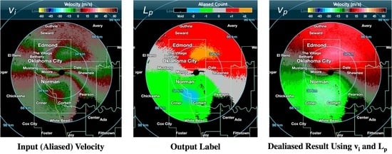
Figure 12.
Similar to Figure 11, this figure shows an example PPI scan with isolated storms observed at . The data are synthesized using a 1.32°-EL scan from the KTLX on 30 April 2017 19:14 UTC. The CNN method successfully dealiased the scan as it processed the entire scan all at once. The region-based method, however, failed at a number of isolated storms, which are indicated in the yellow circle. In this example, CNN method predicts the 99.5% on , 99.4% on , and 100% on , while the region-based method predicts 77.9%, 67.8%, and 84.4% on , , and for each.


Table 1.
The number of training, validation, and test scans for mostly filled precipitation and sparsely filled precipitation.
Table 1.
The number of training, validation, and test scans for mostly filled precipitation and sparsely filled precipitation.
| Training | Validation | Test | |
|---|---|---|---|
| Mostly filled precipitation | 240 | 75 | 102 |
| sparsely filled precipitation | 1632 | 240 | 393 |
| Total | 1872 | 315 | 495 |
Table 2.
The population ratio of each label (, , and ) of three different evaluation groups, i.e., , , and .
Table 2.
The population ratio of each label (, , and ) of three different evaluation groups, i.e., , , and .
| 109 | 47.8 | 1 | |
| 6.89 | 1 | 0 | |
| 119 | 1 | 0 |
Table 3.
Comparisons of , , , and between the proposed CNN and the conventional region-based methods. Both methods perform equally well under conditions with mostly filled precipitation. However, under conditions with sparsely filled precipitation, the CNN model outperforms the region-based method.
Table 3.
Comparisons of , , , and between the proposed CNN and the conventional region-based methods. Both methods perform equally well under conditions with mostly filled precipitation. However, under conditions with sparsely filled precipitation, the CNN model outperforms the region-based method.
| (%) | (%) | (%) | (%) | ||
|---|---|---|---|---|---|
| CNN | 99.58 | 99.62 | 97.89 | 93.44 | |
| Mostly Filled | Region-Based | 99.90 | 99.87 | 98.54 | 94.30 |
| Difference | −0.32 | −0.25 | −0.65 | −0.86 | |
| CNN | 99.23 | 98.39 | 96.85 | 84.96 | |
| Sparsely Filled | Region-Based | 96.39 | 96.88 | 91.45 | 74.39 |
| Difference | 2.84 | 1.51 | 5.39 | 10.57 |
Table 4.
Evaluation weights of the different groups and label sets used in Equation (10). The weight is the inverse of the population ratio of each group. As expected, the sum of the weights within each label set is always equal to one.
Table 4.
Evaluation weights of the different groups and label sets used in Equation (10). The weight is the inverse of the population ratio of each group. As expected, the sum of the weights within each label set is always equal to one.
| Group | ||||
|---|---|---|---|---|
| 0.25 | 0.61 | 1.00 | ||
| Mostly Filled | 0.33 | 0.35 | - | |
| 0.42 | 0.04 | - | ||
| 0.28 | 0.74 | 1.00 | ||
| Sparsely Filled | 0.35 | 0.25 | - | |
| 0.38 | 0.01 | - |
Disclaimer/Publisher’s Note: The statements, opinions and data contained in all publications are solely those of the individual author(s) and contributor(s) and not of MDPI and/or the editor(s). MDPI and/or the editor(s) disclaim responsibility for any injury to people or property resulting from any ideas, methods, instructions or products referred to in the content. |
© 2023 by the authors. Licensee MDPI, Basel, Switzerland. This article is an open access article distributed under the terms and conditions of the Creative Commons Attribution (CC BY) license (https://creativecommons.org/licenses/by/4.0/).
Share and Cite
MDPI and ACS Style
Kim, H.; Cheong, B. Robust Velocity Dealiasing for Weather Radar Based on Convolutional Neural Networks. Remote Sens. 2023, 15, 802. https://doi.org/10.3390/rs15030802
AMA Style
Kim H, Cheong B. Robust Velocity Dealiasing for Weather Radar Based on Convolutional Neural Networks. Remote Sensing. 2023; 15(3):802. https://doi.org/10.3390/rs15030802
Chicago/Turabian StyleKim, Hyeri, and Boonleng Cheong. 2023. "Robust Velocity Dealiasing for Weather Radar Based on Convolutional Neural Networks" Remote Sensing 15, no. 3: 802. https://doi.org/10.3390/rs15030802
Note that from the first issue of 2016, this journal uses article numbers instead of page numbers. See further details here.